Econometric Modeling and Model Falsification

(1)

ISSN Online: 2160-0384 ISSN Print: 2160-0368

DOI: 10.4236/apm.2019.99036 Sep. 16, 2019 762 Advances in Pure Mathematics

Econometric Modeling and Model Falsification

George M. Lady

1

_{, Carlisle E. Moody}

2*

1_{Department of Economics, Temple University, Philadelphia, PA, USA}

2_{Department of Economics, College of William and Mary, Williamsburg, VA, USA}

Abstract

A recent literature on qualitative analysis has shown that its successful appli-cation in testing the consistency of the sign patterns of a proposed structure and an estimated reduced form was far less restricted than a previous litera-ture had proposed. A frequent example used in this demonstration was the qualitative analysis of Klein’s Model I. For this, the proposed structural sign pattern was falsified by the sign pattern of the estimated reduced form. As a result, the subsequent application two-stage least squares would always find quantifications of the structure that could not possibly have resulted in the sign pattern of the estimated reduced form. We view this result as a diagnos-tic calling for further analysis. We show that the Klein model fails standard over identification tests. We make modest amendments to the model that re-solves this problem but find that the resulting estimated reduced form still falsifies the structure, calling for further developmental effort. Our point is that qualitative falsification should be viewed as a diagnostic in developing a model, rather than a criterion for entirely dismissing the model.

Keywords

Econometric Modeling, Falsification, Qualitative Analysis

1. Introduction

The issue of the scientific nature of economic theory is surprisingly undeveloped; or, at least, not fully formulated. To set up the issues at stake, we will follow Sa-muelson [1] and later writers in econometrics, e.g., Berndt [2]. In these terms, the theory concerning some aspect of economic activity, i.e., a model, is ex-pressed by a system of simultaneous equations,

(

,

)

0, 1,2, , ,

i

f Y Z = i= _ n ₍₁₎ where Y is an n-vector of endogenous variables and Z is an m-vector of exogen-How to cite this paper: Lady, G.M. and

Moody, C.E. (2019) Econometric Modeling and Model Falsification. Advances in Pure Mathematics, 9, 762-776.

https://doi.org/10.4236/apm.2019.99036

Received: August 8, 2019 Accepted: September 13, 2019 Published: September 16, 2019

http://creativecommons.org/licenses/by/4.0/

(2)

DOI: 10.4236/apm.2019.99036 763 Advances in Pure Mathematics ous variables. This system is brought to the data by the method of comparative statics, as expressed by the total differentiation of the system (1),

1 1

d d 0, 1,2, , .

i i

n m

j k

j j k k

f _y f _z _i _n

y z

= =

∂ ₊ ∂ ₌ ₌

∂ ∂

∑

 (2)

For purposes of estimation, it is usual to assume that (1) is (at least locally) li-near, so that (2) can be more compactly expressed as,

,

Y Z U

β

=

γ

+

δ

(3) where β, γ and δ are appropriately dimensioned matrices, with δU representing errors embodied in the data. The system (3) is termed the structural form of the model. Estimation then proceeds with respect to the reduced form,

,

Y =

π

Z+

ψ

U ₍₄₎ where in (4) _{π β γ}₌ −1 _{. The arrays β and γ are then recovered from the}

esti-mated π using some version of multi-stage least squares. Depending upon issues of identification, there may be more than one way to do this for an over-identified system and no way to do this for an under-identified system.

For the theory to be “scientific”, the expression of the structure (3) must take a form such that the outcomes for the estimate of π are in some way limited. If the outcome of the estimation is not consistent with such limit(s), then the model has been falsified, i.e., Popper [3].

So far, the issues at stake seem straight-forward. Nevertheless, problems arise in terms of what it is about a proposed structure that is hypothesized by the theory; and, given this, just what limits does the hypothesis create for the esti-mated reduced form? Before providing his answers to these questions, Samuel-son ([1] p. 23) considers what he terms “A Calculus of Qualitative Relations”. Typically the theory does not fully quantify the entries of the structural arrays; instead, it only proposes their sign patterns determining the directions of influ-ence among the variables. Given this, it may be possible to “sign” entries of the reduced form by working through the algebra of computing _{π β γ}₌ −1 _{. For this,}

the analytic burden relates to showing that the sign pattern of β requires that at least some entries of the sign pattern of β−1_{must have particular signs,} indepen-dent of the magnitudes of the nonzero entries of β. In fact, much of the subse-quent literature on what has become known as qualitative analysis treats the special case where γ = I, since if any entries of β−1_{can be signed based upon the} sign pattern initially hypothesized for β, it is reasonably easy, given whatever the sign pattern of γ is initially proposed to be, to see if any entries of π can be signed. The Monte Carlo approach identified below will readily detect any sign-able entries of the reduced form, i.e., by showing such entries always have the same sign, based upon the hypothesized sign pattern of the structure. If entries of π can be signed, then the hypothesized sign patterns of the structural arrays are “scientific”, since the hypothesis can be falsified, if the required signs do not show up in the estimated reduced form.

(3)

DOI: 10.4236/apm.2019.99036 764 Advances in Pure Mathematics finding that all of the (potentially millions) of terms in the expansions of β’s de-terminant and (at least some) cofactors would all have the same sign was too small to be taken seriously. Hence, a qualitative analysis of a model’s structure would virtually never yield entries in the reduced form that had to have particu-larly signs and hence (potentially) lead to the falsification of the structural hy-pothesis. Instead, Samuelson proposed that for β derived from the second order conditions of a (possibly constrained) optimization problem, the first n entries of β−1_{’s main diagonal would have to be negative and, for β a stable matrix with} non-negative off-diagonal and negative main diagonal entries, β−1_{would have all} negative entries, e.g., Hale, et al. ([4], p. 148). This could be potentially falsified by the sign pattern of the estimated reduced form. A literature on the conditions under which a qualitative analysis would be successful was initiated by Lancaster [5] and is well-summarized in Hale, et al. [4]. None of this dispelled Samuelson’s pessimism about the potential for a successful qualitative analysis, although Hale and Lady [6] is a significant exception. It is fair to say that such analyses are sel-dom performed and, if so, selsel-dom found to be successful.

A recent literature, Buck and Lady [7] [8] and Lady and Buck [9], has shown that the concept of a qualitative analysis as discussed above was too restrictive. Specifically, it was shown that although no sign in the reduced form could be signed, based upon the sign patterns of the structural arrays; nevertheless, there were (always) restrictions on what sign patterns that the reduced form could take. Given this, if the estimated reduced form took on a sign pattern forbidden by these restrictions, the proposed structural arrays are thereby falsified. As a simple example, for the case that γ = I and β−1_{= π, the sign pattern of the} esti-mated reduced form must be such that it is possible that βπ = I and πβ = I. Given this, the entries of the first row of the estimated reduced form π cannot, for ex-ample, all be the negative of the corresponding nonzeros proposed for the first column of β. This result holds even if no entries of the reduced form can be signed. If the estimated reduced form does not satisfy this restriction, the struc-tural hypothesis has been falsified. Buck and Lady [7] [8] and Lady and Buck [9] describe a Monte Carlo technique for sampling quantitative realizations of the structural arrays and the corresponding reduced form that will identify such re-strictions.

Buck and Lady [10] showed that the scope of restrictions due to a hypothe-sized qualitative structure was even broader than previously proposed. In partic-ular, they showed that falsifiable restrictions on the reduced form can be im-posed by the zero, and perhaps other, restrictions on the structure, independent of the (unrestricted) nonzero entries. As an example, consider the structure γ = I and,

? 0 0 ? ? ? 0 0 . 0 ? ? 0 0 0 ? ? β

 

 

=

 

(4)

DOI: 10.4236/apm.2019.99036 765 Advances in Pure Mathematics In the above array, the entries marked “?” are nonzero, but may otherwise be of any sign and magnitude. The zero restrictions selected present an irreducible inference structure with only one cycle of inference. The Monte Carlo sampling and derivation of the reduced form for β−1_{= π, found only 256 sign patterns out} of the possible 65,536 sign patterns that a 4 × 4 array could take on, barring ze-ros. This result is due to the zero restrictions only and is independent of the nonzero signs and magnitudes of the other entries. Suppose a multistage least squares process were applied to this structure to estimate the nonzero entries. If any but the 256 reduced form sign patterns consistent with the structure were then found in the estimated reduced form, the resulting estimates of the nonze-ros in the structure would be impossible, i.e., could not possibly generate a re-duced form with the sign pattern found in the estimated rere-duced form. Conse-quently, any estimates of the structural nonzeros would be incorrect, since the zero restrictions themselves have been falsified.

One of the examples of falsification due to zero and other restrictions given in Buck and Lady [10] is the Klein [11] Model I. This formulation has been a pop-ular example for pedagogical purposes in econometrics, e.g., Berndt [2]. It has also been used as an example for qualitative analysis, e.g., Maybee and Weiner [12] and Lady [13]. Buck and Lady [10] showed that the sign pattern of the re-duced form estimated by Goldberger [14] and used by Berndt [2] falsified the zero and other restrictions on the model’s structural form, independent of the signs and magnitudes of the nonzero behavioral entries of the structural arrays. However, this in itself is not a decisive finding. It turns out that Klein’s Model 1 fails the Sargan [15] overidentification test for two out of three estimated equa-tions.

In this paper we re-specify the original Klein Model I slightly, but enough to cause it to pass the overidentification tests and re-examine the resulting sign pattern on the theory that the model generated an impossible sign pattern be-cause it was not properly identified in the first place. In the next section Klein’s Model I is briefly reiterated. In Section III, we test the original model’s identifi-cation strategy and suggest a slightly modified version that at least passes the usual overidentification tests. Nevertheless, we found that the zero and other re-strictions on the structural arrays were again falsified by the sign pattern of the reduced form estimated for this case. Therefore, we suggest that the Monte Carlo sign pattern test presented in Buck and Lady (2016) is a complement to rather than a substitute for standard overidentification tests. Unlike Buck and Lady (2016), in the Appendix we go on to find the particular feature of the reduced form sign pattern that falsify the structural arrays and write out the expansions of the corresponding cofactors of Klein’s coefficient matrix that confirm this re-sult. Conclusions are provided in Section 4.

2. Klein’s Model I

(5)

DOI: 10.4236/apm.2019.99036 766 Advances in Pure Mathematics given below,

β

Y=

γ

Z_{, where}

1 2 1 3

1 2 3

1 1 2 3

1 0 0 0 0 0 0 0 0 0

0 1 0 0 0 0 0 0 0 0 0

0 0 1 0 0 0 0 0 0 0 0

1 1 0 1 0 0 0 0 0 0 0 0 1 1

0 0 0 1 1 1 0 0 0 0 0 0 0 0

0 0 1 0 0 1 0 1 0 0 0 0 0 0

0 0 0 1 0 0 1 1 0 0 0 0 1 0

a a C a a

b I b b

c W c c

Y P W E − − −        ₋     ₋ ₋         −     − −   ₋    ₌ ₋         _{− −}            − −        ₋     ₋        2 1 1 1 W P K E Year TX G − − −                      

In this structure the endogenous variables are: private consumption (C), in-vestment (I), the private wage bill (W1), income (Y), profits or nonwage income (P), the sum of private and government wages (W), and private product (E); the exogenous variables are the government wage bill (W2), lagged profits (P−1), end of last period capital stock (K−1), lagged private product (E−1), years since 1931 (Year), taxes (TX), and government consumption (G). The entries notated ai, bj and ck are nine in number and represent the behavioral entries of the model that (ultimately) would be estimated via multi-stage least squares. The remaining en-tries in the structure are restrictions. The sign patterns proposed by Klein for the structural arrays are given by,

0 0 0 0

0 0 0 0 0

sgn 0 0 0 0

0 0 0 0

0 0 0 0 0

β − + +    ₋ ₊     − +   = + +_ − _  _{+ − −}    + −    ₊ ₋   and

0 0 0 0 0

sgn 0 0 0 0 0 .

0 0 0 0 0 0 0 0 0 0 0 0 0

0 0 0 0 0

γ − −    _{− +}     − −    =_ + −_     −   ₊ ₋   

An estimate of the reduced form for this model was provided by Goldberger [14]. The sign pattern of this estimated reduced form is given below,

ˆ

Estimated sgnπ .

− + − + + − +   _{− + − − + − +}   − + − + + − +   = − + − + + − +_ _ _{− + − + + − +}   − + − + + − +   _{− + − + + − +}  

(6)

DOI: 10.4236/apm.2019.99036 767 Advances in Pure Mathematics 0 ? 0 ? 0 0

0 0 0 ? 0 0

0 0 0 0 0 ?

sgn 0 0 0 0

0 0 0 0

0 0 0 0 0

β

−

 

 ₋ 

 

 − 

 

= + +_ − _

 _{+ − −} 

 

+ −

 

 ₊ ₋

 

and

? ? 0 0 0 0 0 0 ? ? 0 0 0 0 0 0 0 ? ? 0 0

sgn 0 0 0 0 0 ,

0 0 0 0 0 0 0 0 0 0 0 0 0

0 0 0 0 0

γ

 

 

=_ + −_

 

−

 

₊ ₋ 

 

there did not exist nonzero signs and magnitudes that could be given to the structural entries marked “?” in the above that would result in the sign pattern of the estimated reduced form. As a result, all of the estimates given in Berndt [2] are impossible.

Thus, Klein Model I generates a sign pattern that is impossible given the sign pattern of the reduced form equations. However, could this sign pattern be a feature of the way in which the model is specified? If the model is not properly identified, then it is not a proper reduction from the reduced form. See Hendry ([16], 421-434). In that case, the impossible sign pattern may be the result of an improper identification strategy. If so, then it might be possible to re-specify the model such that it is properly identified and thereby generate a feasible sign pat-tern. In the following section we test the identification strategy of the original Klein model, find it wanting, and specify a slightly different version of it that at least appears to be a valid reduction from the reduced form.

3. Is Klein Model I Properly Identified?

The Klein Model I is specified, for estimation purposes as follows (Goldberger 1964, 303-304). The variables are defined above.

Klein Model I

1) C a= 0+a P a P1 + 2 −1+a W W3

(

1+ 2

)

+u1

2) I b b P b P= 0+ 1 + 2 −1+b K3 −1+u2 3) W c c E c E1= 0+ 1 + 2 −1+c Year u3 + 3 4) Y C I G TX= + + −

5) P Y W= − 6) W W W= 1+ 2 7) E Y W TX= − 2+

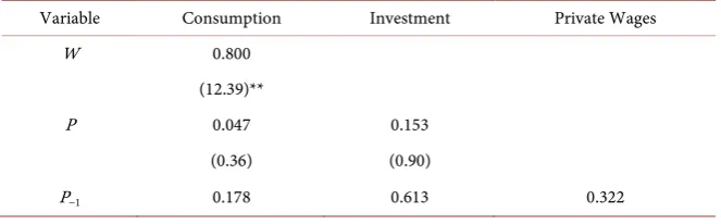
Estimating the three behavioral equations using two-stage least squares yields the results shown in Table 1.

(7)

DOI: 10.4236/apm.2019.99036 768 Advances in Pure Mathematics A bit of experimentation yields the following alternative model, which we call the Klein-Lady-Moody model (KLM). There are only two small changes in be-havioral Equation (2) and Equation (3). In the investment Equation (2’) we have added lagged wages, on the theory that, for example, a rise in wages in the pre-vious year could impinge on investment in the current year. In the private sector wage bill equation we have added taxes, which could reduce employment and/or wages in that sector.

KLM model

1) C a= 0+a P a P1 + 2 −1+a W W3

(

1+ 2

)

+u1

2’) I b b P b P= 0+ 1 + 2 −1+b K3 −1+b W4 −1+u2 3’) W c c E c E1= 0+ 1 + 2 −1+c Year c TX u3 + 4 + 3 4) Y C I G TX= + + −

5) P Y W= − 6) W W W= 1+ 2 7) E Y W TX= − 2+

Using the above notation, the amended model is expressed by,

3 1

1

1 1

3 2

2 3 4

1 0 0 0 0

0 1 0 0 0 0

0 0 1 0 0 0

1 1 0 1 0 0 0

0 0 0 1 1 1 0

0 0 1 0 0 1 0

0 0 0 1 0 0 1

0 0 0 0 0 0

0 0 0 0 0

0 0 0 0 0 1 1 0

0 0 0 0 0 0 0 0

1 0 0 0 0 0 0 0

1 0 0 0 0 1 0 0

a a C

b I c W Y P W E a a

b b b

c c c

−      ₋         −     ₋         ₋ ₋        −      ₋        − −   ₋ ₋ ₋   − − −  =_ −   −   ₋  2 1 1 1 1 W P K E Year TX G W − − − −                                  _ _

In writing out the expansions of the entries of π referred to in falsifying the KLM version of the model given in the Appendix, the above notation is used.

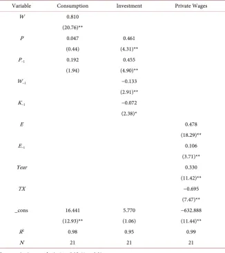
[image:7.595.209.541.624.727.2]

The resulting estimated KLM behavioral equations are presented in Table 2.

Table 1. Klein model I behavioral equations.

Variable Consumption Investment Private Wages

W 0.800

(12.39)**

P 0.047 0.153

(0.36) (0.90)

(8)

DOI: 10.4236/apm.2019.99036 769 Advances in Pure Mathematics

Continued

(1.10) (3.83)** (1.89)

E−1 0.014 0.083

(0.20) (1.30)

K−1 −0.157

(4.40)**

E 0.330

(5.30)**

Year 0.303

(4.41)**

_cons 16.250 20.181 −579.702

(9.20)** (2.71)** (4.43)**

R2 _0.98 _0.89 _0.97

N 21 21 21

[image:8.595.210.537.351.718.2]

Note: t-ratios in parenthesis; *p < 0.05; **p < 0.01.

Table 2. KLM model behavioral equations.

Variable Consumption Investment Private Wages

W 0.810

(20.76)**

P 0.047 0.461

(0.44) (4.31)**

P−1 0.192 0.455

(1.94) (4.90)**

W−1 −0.133

(2.91)**

K−1 −0.072

(2.38)*

E 0.478

(18.29)**

E−1 0.106

(3.71)**

Year 0.330

(11.42)**

TX −0.695

(7.47)**

_cons 16.441 5.770 −632.888

(12.93)** (1.06) (11.44)**

R2 _0.98 _0.95 _0.99

N 21 21 21

(9)

DOI: 10.4236/apm.2019.99036 770 Advances in Pure Mathematics The Sargan overidentification test statistics are no longer significant: consump-tion (p = 0.0782), investment (p = 0.0993), private wages (p = 0.1117). Thus, whatever else might be said about this model, it appears to be a valid reduction from the reduced form. The resulting matrix representation of the KLM model is as follows.

1

1 0 0.810 0 0.047 0 0

0 1 0 0 0.461 0 0

0 0 1 0 0 0 0.478

1 1 0 1 0 0 0

0 0 0 1 1 1 0

0 0 1 0 0 1 0

0 0 0 1 0 0 1

0.810 0.192 0 0 0 0 0 0

0 0.455 0.072 0 0 0 0 0.113

0 0 0 0.106 0.330 0.695 0 0

0 0 0 0 0 1 1 0

0 0 0 0

C I W Y P W E −      ₋         −     ₋         ₋ ₋        −      ₋        − − − − − = − 2 1 1 1 1

0 0 0 0

1 0 0 0 0 0 0 0

1 0 0 0 0 1 0 0

W P K E Year TX G W − − − −    _{ } _  _{ } _  _{ }   _{ } _  _{ } _  _{ } _  _{ }   _{ } _ −  _{ } _  ₋ _{ } _  _{ } _  

0 0 0 0

0 0 0 0 0

sgn 0 0 0 0

0 0 0 0

0 0 0 0 0

β − + +    ₋ ₊     − +   = + +_ − _  _{+ − −}    + −    ₊ ₋   ,

0 0 0 0 0 0

0 0 0 0 0

sgn 0 0 0 0 0 0

0 0 0 0 0 0 0 0 0 0 0 0 0 0 0

0 0 0 0 0 0

γ − −    _{− +} ₊    − − +    =_ + − _     −   ₊ ₋   

Does this solve the impossibility issue? We use the same Monte Carlo metho-dology reported on in Buck and Lady [10] to determine whether this sign pat-tern is possible. A version of the computer application that implements the Monte Carlo that we used is available at

https://astro.temple.edu/~gmlady/RF_Finder/Finder_Page.htm which also

con-tains the Stata programs and data used to estimate the models presented herein. The reduced form estimated for the KLM model is given below in Table 3. The Monte Carlo method takes quantitative samples of the structural arrays with the sign patterns given above, computes _{π β γ}₌ −1 _{, and then checks to see}

if the resulting sign pattern of π as computed from the sample corresponds to the sign pattern of the estimated reduced form given above. The sample is con-structed as follows.

(10)

Table 3. KLM estimated reduced form.

W2 P−1 K−1 E−1 Year TX G W−1

C 1.164807 1.103044 −0.0808039 0.3888034 0.7563496 −0.2291788 0.208483 −0.6608964 I 0.1787256 1.091179 −0.1319317 0.1959241 0.382831 −0.0356712 0.1034288 −0.7714421 W1 0.4761662 1.146809 −0.0607081 0.3068805 0.7659097 −0.4748558 0.8695093 −0.6870231 P 0.8673651 1.047414 −0.1520275 0.2778469 0.3732713 −0.7899943 0.4424027 −0.7453154 Y 1.343533 2.194224 −0.2127355 0.5847274 1.139181 −0.2648502 1.311912 −1.432339 W 1.476168 1.14681 −0.0607081 0.3068805 0.765909 −0.4748559 0.8695091 −0.6870232

E 0.3435363 2.194224 −0.2127354 0.5847274 1.13918 0.7351493 1.311912 −1.432339

form, the sign pattern of which is then compared to the sign pattern of the esti-mated reduced form. Call the sign patterns proposed for beta and gamma the text-files and the particular quantification chosen the sample-files. The steps in selecting the sample-files from the text-files are as follows.

1) The text files for β and γ are read into their corresponding sample arrays. 2) All entries in the sample-files are set equal to zero if the corresponding en-tries in the text-files are equal to zero, preserving the zero restrictions.

3) The value of each remaining (not set to zero) entry of the sample-files are chosen individually and randomly from the open interval (0, 100) using a uni-form distribution.

4) The values in the sample-files chosen in step 2) above that correspond to negative entries in the text-files are set negative.

5) The value of γ(1, 1) in the sample file is set equal to the negative of β(1, 3) in the sample-file, a restriction of both the Klein Model I and the KLM structural form.

6) All entries other than β(1, 1) that are equal to “1” or “−1” in the structural form are set equal to the absolute value of the value with chosen for beta (1, 1) in the sample file, keeping their appropriate sign as given in the text-files.1

The sample-files are then used to compute the implied reduced form, the sign pattern of which is compared to the sign pattern of the estimated reduced form. Subject to the precision of the real variables utilized by the computer software being used (Visual Basic Version 6, service pack 6), the sample-files would in principle allow any possible quantification of the text-files with the given sign patterns and structural form restrictions.

1,6

( )

2,6 .

π =π +π

The derivation of this result is given in the Appendix. Further study revealed that this result could be readily derived from the system of equations. For

2

dTX ≠0, dG=dW =0_{, the result found can be expressed by the condition,}

dE=dC+d .I From Equation (7),

dE=dY+d ;TX and from Equation (4),

dY =dC+dI−dTX.

Substituting this into the relationship from Equation (7) yields, dE=dC+d .I

the result derived from the expansions involved in the computation of _{π β γ}₌ −1 _.

Accordingly, this condition can only be satisfied if sgnπ

( )

7,6 equals (at least) one of (sgn 1,6π

( )

, sgnπ

( )

2,6 ). Thus, the signs of this triplet of entries in the estimated reduced form falsifies the model, i.e., are impossible. Further, this re-sult is based entirely upon the accounting relationships (4) and (7) and is there-fore independent of the signs and values of the behavioral coefficients. Thus, al-though our amendments to Klein’s original specification solved the overidenti-fication problem, the model is nevertheless falsified and is falsified independent of the signs and values of the behavioral coefficients.

4. Conclusions

(12)

DOI: 10.4236/apm.2019.99036 773 Advances in Pure Mathematics demonstration presented here was to react to the falsification of the original Klein Model I, as presented in Buck and Lady [10], and test the model for over-identification, which we found was present. Given this, we introduced some modest amendments to the original model, yielding our version, the KLM model. These amendments resolved the overidentification problem, but further analysis revealed that, nevertheless, the KLM model was also falsified by the estimated reduced form sign pattern. Significantly, the model was falsified based upon the zero and other restrictions, with the finding independent of either the signs or magnitudes of the behavioral coefficients of the model, i.e., the falsification was based upon accounting relationships embodied in the model’s structural forms.

Our point is then that such a finding should prompt additional analysis in the further development of the model’s structural form and the underlying data upon which the model is based. The important point is that, among other tests, a qualitative analysis could provide a useful analytical tool to support development. The Monte Carlo technique utilized for this analysis is easily programmed into a spread sheet and can readily reveal what reduced form sign patterns (appear) possible, among other things based only upon the structural form’s restrictions. In our opinion, when these restrictions are falsified by the estimated reduced form sign pattern, further development is appropriate and initiating the second stage of two stage least squares is not.

Conflicts of Interest

The authors declare no conflicts of interest regarding the publication of this pa-per.

References

[1] Samuelson, P. (1947) Foundations of Economic Analysis. Harvard University Press, Cambridge.

[2] Popper, K. (1959) The Logic of Scientific Discovery. Harper and Row, New York. [3] Berndt, E. (1996) The Practice of Econometrics: Classic and Contemporary.

Addi-son-Wesley Publishing Co., Boston.

[4] Hale, D., Lady, G., Maybee, J. and Quirk, J. (1999) Nonparametric Comparative Statics and Stability. Princeton University Press, Princeton.

[5] Lancaster, K. (1962) The Scope of Qualitative Economics. Review of Economic Stu-dies, 29, 99-132.https://doi.org/10.2307/2295817

[6] Hale, D. and Lady, G. (1995) Qualitative Comparative Statics and Audits of Model Performance. Linear Algebra and Its Applications, 217, 141-154.

https://doi.org/10.1016/0024-3795(94)00125-W

[7] Buck, A. and Lady, G. (2012) Structural Sign Patterns and Reduced Form Restric-tions. Economic Modelling, 29, 462-470.

https://doi.org/10.1016/j.econmod.2011.12.003

[8] Buck, A.J. and Lady, G.M. (2015) A New Approach to Model Verification, Falsifica-tion and SelecFalsifica-tion. Econometrics, 3, 466-493.

(13)

[9] Lady, G. and Buck, A. (2011) Structural Models, Information and Inherited Restric-tions. Economic Modelling, 28, 2820-2831.

https://doi.org/10.1016/j.econmod.2011.08.021

[10] Buck, A.J. and Lady, G.M. (2016) Estimating a Falsified Model. Advances in Pure Mathematics, 6, 523-531.https://doi.org/10.4236/apm.2016.68040

[11] Klein, L. (1950) Economic Fluctuations in the U.S. 1921-1941. Cowles Commission for Research in Economics Monograph No. 11, John Wiley and Sons, New York. [12] Maybee, J. and Weiner, G. (1988) From Qualitative Matrices to Quantitative

Re-strictions. Linear and Multilinear Algebra, 22, 229-248. https://doi.org/10.1080/03081088808817837

[13] Lady, G. (2000) Topics in Nonparametric Comparative Statics and Stability. Inter-national Advances in Economic Research, 5, 67-83.

https://doi.org/10.1007/BF02295752

[14] Goldberger, A.S. (1964) Econometric Theory. John Wiley & Sons, New York. [15] Sargan, J.D. (1958) The Estimation of Economic Relationships Using Instrumental

( ) ( )

4

3 1

)

;

a =a c a+ −a

and,

( )

1,7 1 3

(

1 1

)

1 1;

a =c a −b −c a

so that,

( ) ( )

4 1 4 3 4 3 1 1 1 3 1

det β π 1,6 =c a c a− +c a b a c a b+ + .

4 3 1 4 1 1 1 1 1 1 3 1 1

det β π 2,6 = −c a b c b b c b c b a+ + − − +c b.

( )

7,3 3 1 1;

a =a b a− −

( )

7,4 1;

a =

and,

( )

7,7 1 1 1;

(15)

DOI: 10.4236/apm.2019.99036 776 Advances in Pure Mathematics so that,

( ) ( )

4 1 4 1 4 3 1 1

det β π 7,6 =c b c a c a+ − +a b+ .

Based on these expansions, the reader can quickly verify that,

( ) ( )

4 1 4 1 4 3 1 1

det β π 1,6 +det β π 2,6 =det β π 7,6 =c b c a c a+ − +a b+ .