Advance Access publication 2017 October 11
The open flux evolution of a solar-mass star on the main sequence
V. See,
1,2‹M. Jardine,
1A. A. Vidotto,
3J.-F. Donati,
4,5S. Boro Saikia,
6,7R. Fares,
8,9C. P. Folsom,
4,5,10,11S. V. Jeffers,
6S. C. Marsden,
12J. Morin,
13P. Petit
4,5and the BCool Collaboration
1SUPA, School of Physics and Astronomy, University of St Andrews, North Haugh, St Andrews KY16 9SS, UK 2Department of Physics and Astronomy, Physics Building, University of Exeter, Stocker Road, Exeter EX4 4QL, UK 3School of Physics, Trinity College Dublin, University of Dublin, Dublin-2, Ireland
4Universit´e de Toulouse, UPS-OMP, Institut de Recherche en Astrophysique et Plan´etologie, F-31400 Toulouse, France 5CNRS, Institut de Recherche en Astrophysique et Plan´etologie, 14 Avenue Edouard Belin, F-31400 Toulouse, France 6Universit¨at G¨ottingen, Institut f¨ur Astrophysik, Friedrich-Hund-Platz 1, D-37077 G¨ottingen, Germany
7Institut f¨ur Astronophysik, Universit¨at Wien, T¨urkenschanzstrasse 17, A-1180 Wien, Austria 8INAF-Osservatorio Astrofisico di Catania, Via Santa Sofia, 78, I-95123 Catania, Italy
9Department of Natural Sciences, School of Arts and Sciences, Lebanese American University, PO Box 36, Byblos, Lebanon 10Univ. Grenoble Alpes, IPAG, F-38000 Grenoble, France
11CNRS, IPAG, F-38000 Grenoble, France
12Computational Engineering and Science Research Centre, University of Southern Queensland, Toowoomba, 4350 Queensland (QLD), Australia 13Laboratoire Univers et Particules de Montpellier, Universit´e de Montpellier, CNRS, F-34095 Montpellier, France
Accepted 2017 October 4. Received 2017 September 29; in original form 2017 March 27
A B S T R A C T
Magnetic activity is known to be correlated to the rotation period for moderately active main-sequence solar-like stars. In turn, the stellar rotation period evolves as a result of magnetized stellar winds that carry away angular momentum. Understanding the interplay between mag-netic activity and stellar rotation is therefore a central task for stellar astrophysics. Angular momentum evolution models typically employ spin-down torques that are formulated in terms of the surface magnetic field strength. However, these formulations fail to account for the magnetic field geometry, unlike those that are expressed in terms of the open flux, i.e. the magnetic flux along which stellar winds flow. In this work, we model the angular momentum evolution of main-sequence solar-mass stars using a torque law formulated in terms of the open flux. This is done using a potential field source surface model in conjunction with the Zeeman–Doppler magnetograms of a sample of roughly solar-mass stars. We explore how the open flux of these stars varies with stellar rotation and choice of source surface radii. We also explore the effect of field geometry by using two methods of determining the open flux. The first method only accounts for the dipole component while the second accounts for the full set of spherical harmonics available in the Zeeman–Doppler magnetogram. We find only a small difference between the two methods, demonstrating that the open flux, and indeed the spin-down, of main-sequence solar-mass stars is likely dominated by the dipolar component of the magnetic field.
Key words: techniques: polarimetric – stars: activity – stars: evolution – stars: magnetic field – stars: rotation.
1 I N T R O D U C T I O N
Understanding how the angular momentum and rotation periods of low-mass stars (M 1.3 M) evolve over their lifetimes is an important goal within stellar astrophysics. For example,
E-mail:[email protected]
periods have converged on to a single track in the rotation period– age plane (for solar-mass stars, convergence occurs at∼1 Gyr). Finally, the magnetic activity and rotation history of a host star can also have a significant impact on the potential habitability of exo-planets (Wood et al.2014; Tu et al.2015; Ribas et al.2016; Gallet et al.2017). For example, stellar winds can significantly compress planetary magnetospheres (Vidotto et al.2013; See et al.2014) and reduce their ability to protect the planetary atmosphere from the erosive effects of the wind. Planetary atmospheres can also be eroded away by photoevaporation caused by high-energy radiation (Lammer et al.2003). The rate at which this occurs depends strongly on the initial rotation period of the host star (Johnstone et al.2015b). Along the main sequence, the main agent of angular momentum evolution is magnetized stellar winds that carry angular momentum away from the central star. Many authors have studied the rate at which stars lose angular momentum (Cohen & Drake2014; Vidotto et al.2014a; Garraffo, Drake & Cohen2015; Nicholson et al.2016; See et al.2017) or formulated braking laws that describe how the angular momentum loss varies as a function of the parameters of the host star (Matt et al.2012b; Reiners & Mohanty2012; R´eville et al.2015a). These braking laws have subsequently been used to model stellar rotation period evolution from the pre-main sequence (PMS) to ages older than the Sun (Gallet & Bouvier2013,2015; Brown 2014; Johnstone et al. 2015a; Matt et al. 2015; Amard et al.2016; Blackman & Owen2016; van Saders et al.2016).
Numerous studies have shown that the open flux is an impor-tant parameter in the context of angular momentum loss (Mestel & Spruit1987; Vidotto et al.2014a; R´eville et al.2015a,b). However, it is not directly observable and must be estimated using physi-cal models. One such model is the potential field source surface (PFSS) model (Altschuler & Newkirk1969). This model takes an input magnetogram of the stellar surface and extrapolates the field upwards to the so-called source surface; a spherical surface that represents the limit of coronal confinement. Once the source sur-face is reached, the field lines are assumed to be open and radial, mimicking the action of plasma pressure opening up closed field lines.
A number of factors can affect the amount of open flux estimated by the PFSS model. The first is the choice of an input magnetogram. Previous theoretical work has shown that, when considering indi-vidual field modes, stars with dipolar surface fields have the most open flux and that the open flux decreases with increasing spherical harmonic degree (quadrupole, octupole, etc.; Garraffo et al.2015; R´eville et al.2015a). For stellar studies, the input magnetogram is typically a Zeeman–Doppler imaging (ZDI) map (Jardine, Collier Cameron & Donati2002; Gregory et al.2006; Fares et al.2010; Lang et al.2012; Johnstone et al.2014; See et al. 2015a). ZDI is a tomographic technique that is capable of reconstructing the large-scale surface magnetic field structure of cool-dwarf stars (Semel1989; Brown et al.1991; Donati & Brown1997; Donati et al.2006). Over the last two decades, a considerable amount of effort has been dedicated to investigating the field geometry of low-mass stars. It has been found that their surface fields are composed of a mixture of spherical harmonic modes (e.g. Jeffers et al.2014; Boro Saikia et al.2015,2016; Folsom et al.2016). However, recent work suggests that the open flux is dominated by the dipolar com-ponent of the field, at least for the choice of source surface radius used in those works (Lang et al.2014; Jardine, Vidotto & See2017; See et al.2017). This is because the dipolar component of the field decays the most slowly with height above the stellar surface. Given that the ZDI technique can typically reconstruct the stellar magnetic field up to a spherical harmonic mode of, at least,=5, ZDI maps
are an appropriate choice of inner boundary condition for the PFSS model in the context of determining the open flux.
The source surface radius is another parameter that can affect the amount of open flux recovered. Within the PFSS model, it is a free parameter but it is observationally unconstrained for stars other than our Sun. For a given input map, more of the flux is forced to be open for smaller values of the source surface radius. Additionally, if the source surface is sufficiently small, the higher order field modes may not have completely decayed away and may contribute towards the open flux. Typically, the source surface radius is picked to have values similar to the solar value (∼2.5r) but in reality it should vary as a function of the fundamental parameters of the star (R´eville et al.2015b).
In See et al. (2017), we studied how the open flux and the cor-responding spin-down torque varied using a sample of low-mass stars with a wide range of masses and rotation periods. We found that the open flux of stars with Rossby numbers, Ro, greater than
∼0.01 follows the classical activity rotation relation shape but that Ro0.01 stars departed from this relation. These results were ob-tained using the simplifying assumption that all the stars had source surface radii ofrss=3.41r. This is a useful assumption since it
allows for a rapid assessment of how stellar open flux varies over a large portion of the HR diagram. However, it ignores the fact that the source surface radius likely varies as a function of mass and rotation period. Indeed, to these authors’ knowledge, there has not been a systematic study of how the source surface affects the open flux recovered for a set of realistic input magnetograms to date.
In this study, we will use a sample of 22 main-sequence stars of roughly solar mass (0.9 M<M<1.1 M) which have had their large-scale surface magnetic fields mapped to investigate the open flux evolution main-sequence solar-mass stars. Using a PFSS model, we investigate how the open flux of these stars varies for different source surface radii and the effect of including/excluding higher order field modes. The angular momentum evolution of a solar-mass star can then be calculated over its lifetime using these open flux formulations, in conjunction with the braking law of R´eville et al. (2015a). We use rotation period data from open clusters of known ages to constrain our angular momentum evolution model and determine how the source surface radius and open flux vary over the main-sequence lifetime. In Section 2, we outline the details of our spin-down model. In Section 3, we outline two methods of determining the open flux as a function of rotation and source surface radius. In Section 4, we discuss the open cluster data we use to calibrate our model. In Section 5, we present the results of our angular momentum evolution model. A discussion and the conclusions follow in Section 6.
2 A N G U L A R M O M E N T U M E VO L U T I O N M O D E L
In order to determine how the rotation period of a star evolves, we need to solve the angular momentum equation,
d dt =
˙
J
I −
I
dI
dt , (1)
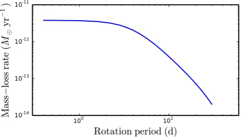
Figure 1. Mass-loss rate against rotation period for a solar-mass star as calculated using the model of Cranmer & Saar (2011).
of a star remains relatively constant on the main sequence and so the changes in angular velocity are dominated by the spin-down torque term in equation (1).
For the spin-down torque, we use the formulation of R´eville et al. (2015a),
˙
JR15=M˙ r2K32
ϒopen
1+f2/K2 4
1/2
2m
, (2)
where ˙M is the mass-loss rate,r is the stellar radius,ϒopen=
2
open/(r 2
Mv˙ esc) is a measure of the magnetization of the open field
lines,openis the open flux,vesc=(2GM/r)1/2is the stellar escape
velocity,Mis the stellar mass,f =r3/2(GM)−1/2is the angu-lar rotation speed normalized to the breakup speed andK3=0.65,
K4= 0.06 andm=0.31 are fit parameters determined from the results of magnetohydrodynamic (MHD) simulations.1We use the model of Cranmer & Saar (2011) to estimate the mass-loss rate. This is a 1D model that estimates the magnitude of the Alfv´en wave energy flux generated by subsurface convective motions. The model tracks this energy flux through the stellar surface and estimates the amount that is deposited as heat in the transition region. It is this heat that is responsible for driving the winds in this model. Many previ-ous studies have shown that magnetic activity scales with rotation. In the model of Cranmer & Saar (2011), this scaling is encapsulated by the magnetic filling factor that is estimated using empirical scaling relations based on previously published data. Fig.1shows the mass-loss rate of a solar-mass star as a function of rotation period using this model. Similarly to other phenomena related to magnetic activ-ity, the mass-loss rate increases with decreasing rotation period and saturates at the fastest rotation periods. In order to estimate the open flux, we will use the PFSS model in conjunction with ZDI maps. Investigating how the open flux varies with rotation and source sur-face radii will form the focus of this work and will be presented in Section 3. Having calculated ˙JR15, we will assume that the real spin-down torque is proportional to this value, i.e. ˙J =kJ˙R15. Such an assumption has also been made in previous works (Gallet & Bouvier 2013,2015; Johnstone et al.2015a). We will fit for the proportionality constant,k, and discuss its physical significance in Section 5. Lastly, Table1contains the solar values that we use in this study.
1The value ofK
3is given as 1.4 by R´eville et al. (2015a). However, this is
a typographical error and the true value isK3=0.65 (R´eville, priv. comm.).
Table 1. Adopted solar values in this study.
M(solar mass) 2.0×1033g
r(solar radius) 6.96×1010cm
Prot,(solar rotation period) 26 d
τc(solar-mass convective turnover time) 14.45 d
Prot,crit(critical rotation period) 1.45 d
rss,(solar source surface radius) 2.5r
t(solar age) 4.6 Gyr
3 E S T I M AT I N G T H E O P E N F L U X
3.1 The PFSS model
In order to estimate the open flux, we use the PFSS model (Altschuler & Newkirk1969). In this model, the magnetic field is assumed to be in a potential state, i.e. current free, and the three components are given by
Br= −
N
l=1
l
m=l
[lalmrl−1−(l+1)b
lmr−(l+2)]Plm(cosθ) eimφ (3)
Bθ= −
N
l=1
l
m=l
[almrl−1+b
lmr−(l+2)] d
dθPlm(cosθ) e
imφ (4)
Bφ= −
N
l=1
l
m=l
[almrl−1+blmr−(l+2)]Plm(cosθ) im sinθe
imφ, (5)
wherelis the spherical harmonic degree,mis the azimuthal number,
almandblmare the amplitudes of each spherical harmonic compo-nent andPlmare the Legendre polynomials. Equations (3)–(5) only apply between the stellar surface and the source surface with the field assumed to decay radially as an inverse square law above the source surface. In order to determine the values ofalmandblm, two boundary conditions are required. The first is the field geometry at the stellar surface which is set using ZDI maps. We use a sample of 22 main-sequence stars with masses between 0.9 and 1.1 M.2 The large-scale surface magnetic fields of each of these stars have been mapped with ZDI, sometimes over multiple epochs. The pa-rameters of these stars are shown in Table2along with a reference to the article their magnetic map was originally published in. The stellar parameters are taken from the same references or Vidotto et al. (2014b) and references therein. It should be noted that values for the stellar parameters have been obtained from a number of different sources which will add systematic consistency errors. The second boundary condition is the requirement that the field must become purely radial at some distance away from the star known as the source surface radius,rss. As discussed in the introduction, the value ofrssis a free parameter in this model. The open flux is then given by integrating the radial field over the source surface
open=
rss
|Br|dS. (6)
2There are a number of reported masses for AB Dor in the literature. Donati,
[image:3.595.307.548.72.151.2]Table 2. Parameters of the stars mapped with ZDI listed in an ascending order of rotation period: stellar mass, radius, rotation period, age, surface dipolar flux, total surface flux, and the source surface radius for which the open flux calculated using the multipolar method differs from the open flux calculated using the dipolar method by 10% (see Sections 3.2 and 3.3). No value is listed for stars for which the dipolar and multipolar open fluxes never differ by more than 10 per cent. The observation epoch at which each star was observed and references for the paper in which the original magnetic map was published are also listed. The stellar parameters are also taken from these references or Vidotto et al. (2014b) and references therein.
Star M r Prot Age ,dip rss,10% Obs Ref.
ID (M) (r) (d) (Myr) (1023Mx) (1023Mx) (r
) epoch
AB Dor 1a 1 0.51 120 34.65 79.76 1.84 2001 Dec Donati et al. (2003a)
– – – – – 44.31 65.15 1.45 2002 Dec –
PELS 031 0.95 1.05 2.5 125 4.90 11.65 2.51 2013 Nov Folsom et al. (2016)
HII 296 0.9 0.93 2.61 125 25.72 27.69 – 2009 Oct Folsom et al. (2016)
BD-16351 0.9 0.88 3.21 42 14.62 15.55 – 2012 Sept Folsom et al. (2016)
HD 166435 1.04 0.99 3.43 3800 1.88 6.53 4.05 – Petit et al. (in preparation)
HD 175726 1.06 1.06 3.92 500 2.40 4.71 2.11 – Petit et al. (in preparation)
V 447 Lac 0.9 0.81 4.43 257 2.50 4.17 2.83 2014 Jun Folsom et al. (2016)
HN Peg 1.085 1.04 4.6 260 6.05 7.06 1.33 2007 Jul Boro Saikia et al. (2015)
– – – – – 2.96 4.65 1.76 2008 Aug –
– – – – – 4.39 5.91 1.33 2009 Jun –
– – – – – 5.44 7.30 1.29 2010 Jul –
– – – – – 4.56 7.72 2.06 2011 Jul –
– – – – – 8.17 9.46 1.13 2013 Jul –
TYC 5164-567-1 0.9 0.89 4.68 120 22.57 23.51 – 2013 Jun Folsom et al. (2016)
HD 39587 1.03 1.05 4.83 500 2.75 6.64 2.18 – Petit et al. (in preparation)
HIP 12545 0.95 1.07 4.83 24 40.75 45.62 1.06 2012 Sept Folsom et al. (2016)
HD 72905 1 1 5 500 1.90 4.57 3.23 – Petit et al. (in preparation)
DX Leo 0.9 0.81 5.38 257 7.85 8.48 – 2014 May Folsom et al. (2016)
V 439 And 0.95 0.92 6.23 257 4.31 4.51 – 2014 Sept Folsom et al. (2016)
HD 190771 0.96 0.98 8.8 2700 2.84 3.98 2.09 – Petit et al. (in preparation)
κCeti 1.03 0.95 9.3 600 4.38 6.23 1.85 2012 Oct do Nascimento et al. (2016)
HD 73350 1.04 0.98 12.3 510 1.69 3.44 2.84 – Petit et al. (in preparation)
HD 73256 1.05 0.89 14 830 1.21 2.12 2.66 2008 Jan Fares et al. (2013)
HD 56124 1.03 1.01 18 4500 1.11 1.12 – – Petit et al. (in preparation)
18 Sco 0.98 1.02 22.7 4700 0.42 0.62 2.26 2007 Aug Petit et al. (2008)
HD 9986 1.02 1.04 23 4300 0.33 0.34 – – Petit et al. (in preparation)
HD 46375 0.97 0.86 42 5000 0.81 0.83 – 2008 Jan Fares et al. (2013)
Note.aWe have listed the mass for AB Dor as 1 M
but there have been a range of reported masses for AB Dor in the literature. See the footnote in Section 3.1 for further discussion.
See et al. (2017) showed that for low-mass stars (<1.4 M), the open flux is determined predominantly by the dipolar component of the magnetic field, at least for their chosen source surface radii of rss = 3.41R. In this work, we will investigate whether this
assumption holds for different choices of the source surface radii. We will outline two methods of estimating the open flux of a solar-mass star. The first method will use only the dipolar component of the ZDI maps as inputs to the PFSS model while the second method will use the full set of spherical harmonics available in ZDI maps. We will refer to these as the dipolar and the multipolar methods, respectively.
3.2 Dipolar method of determining open flux
Fig.2shows the surface flux associated with the dipolar component (l=1) of the ZDI maps,, dip, as a function of rotation period. In this work, we will define the unsaturated regime to be Ro>0.1. For solar-mass stars, which have convective turnover times of 14.45 d (calculated using equation 11 of Wright et al. 2011), this corresponds to a critical rotation period ofProt,crit =1.45 d. The fit to the unsaturated stars (those stars with Prot > Prot,crit) has the form ,dip=(6.69±3.28)×1024Prot−1.58±0.23. This fit, as well as the others in this work, was done using the bisector ordinary least-squares method (Isobe et al. 1990). The errors on the fit are determined by considering only the scatter of the
Figure 2. Surface dipolar flux against rotation period. Stars observed at multiple epochs are connected by a vertical line. The fit to the stars in the unsaturated regime (solid blue line,Prot>1.44 d) has the form,dip=
(6.69±3.28)×1024Prot−1.58±0.23. The surface dipolar flux has a value of
3.72×1024Mx in the saturated regime (dashed blue line,Prot<1.44 d).
[image:4.595.311.547.457.655.2]points. From the presently available data, it is difficult to constrain the value of the surface dipolar flux in the saturated regime. Currently, only a single star of roughly solar mass in the saturated regime (AB Dor) has been mapped with ZDI. For now, we will assume that the surface dipolar flux transitions continuously from the unsaturated regime to the saturated regime such that it has a value of 6.69×1024P−1.58
rot,crit=3.72×10
24 Mx. This corresponds well with the surface dipolar flux of AB Dor. However, further ZDI observations of solar-mass stars in the saturated regime will be required to determine if this estimate of dipolar flux in the saturated regime is a representative of the true value.
In general, equations (3) and (6) should be used to calculate the open flux when using all the available spherical harmonics in a ZDI map. However, when considering only the dipolar component of the ZDI map, the open-to-surface flux ratio is simply given by
open,dip
,dip
= 3˜rss2 2˜r3
ss+1
, (7)
where ˜rss=rss/r is the ratio of the source surface radii to the
stellar radii. This simple expression exists because we are dealing with only a single spherical harmonic mode and no cross-terms arise when calculating the integral in equation (6). A full deriva-tion of equaderiva-tion (7) is available in Appendix A. By combining equation (7) with the expression for the surface dipolar flux, as a function of rotation period, derived from Fig.2, we have a simple way of estimating the dipolar open flux of a star as a function of ro-tation period and source surface radii. In this work, we will assume that the source surface radius can be parametrized as
rss=rss,
Prot
Prot,
n
, (Prot> Prot,crit)
rss=rss,
P
rot,crit
Prot,
n
, (Prot< Prot,crit), (8)
where values for the solar source surface radius,rss,, and rota-tion period,Prot,, can be found in Table1andnis a power-law index that we will determine in Section 5. In principle, to prop-erly determine the source surface radius, one should consider the location where the plasma thermal pressure and bulk ram pressure of the wind are able to overcome the magnetic pressure of the field causing the field lines to open up (see R´eville et al.2015b
for an in-depth discussion of how to determine the source surface radius). However, we choose to use the simplified form presented in equation (8). Such a dependence is not unreasonable given that many phenomena associated with stellar activity, such as large-scale magnetic fields (Vidotto et al.2014b; See et al.2015b), mass loss (Cranmer & Saar2011) and X-ray emission (Wright et al.2011), have a power-law dependence on rotation in the unsaturated regime with saturation occurring for the fastest rotators. It should also be noted that the source surface radius of a given star should vary due to various forms of intrinsic variability in the stellar magnetic field such as stellar cycles. These short-term fluctuations are not con-sidered by our model and the value calculated using equation (8) should be regarded as a source surface radius value averaged over evolutionary time-scales.
3.3 Multipolar method of determining open flux
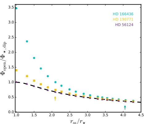
[image:5.595.309.543.52.253.2]In this section, we will estimate the open flux using the full set of spherical harmonics available from the ZDI maps. Unfortunately, there is no simple analytic method of estimating the open flux from the surface flux analogous to equation (7) due to the summation
Figure 3. Open flux normalized to the surface dipolar flux against source surface radii for HD 166435 (cyan circles), HD 190771 (yellow squares) and HD 56124 (purple triangles). Atrss/r=1, the open flux is equal to flux at the stellar surface since all the magnetic flux is forced to be open. The dashed line represents the normalized open flux from a purely dipolar field, i.e. equation (7). Cyan and yellow arrows indicate therss,10%values
for HD 166435 and HD 190771. No arrow is shown for HD 56124 since the discrepancy between the open fluxes determined from the multipolar case and the dipolar case never exceeds 10 per cent.
over different modes in equation (3). We must therefore numerically evaluate equation (6) for a range of source surface radii to determine the impact of the higher order modes on the open flux. Fig.3shows the open flux,open, normalized to the surface dipolar flux,, dip, against source surface radius for three stars from our sample. A dashed line represents the open flux expected in a purely dipolar case, i.e. as calculated by equation (7). The three chosen stars rep-resent three cases. The surface magnetic field of HD 56124 (purple triangles), as determined from ZDI, is strongly dipolar. As such, it follows the pure dipole case (dashed line) very closely. On the other hand, the dipolar component represents only a small fraction of the magnetic energy in the ZDI map of HD 166435 (cyan circles). This star therefore shows large deviations from the pure dipole case at the smallest values ofrss. HD 190771 (yellow squares) represents an intermediate case and is also a representative of the majority of the stars in our sample. From Fig.3, it is clear to see why See et al. (2017) found that the dipole component dominated the open flux for their chosen source surface radii ofrss=3.41r. Even for HD
166435, which has one of the weakest dipole components in our sample, the effects of higher order spherical harmonics have become small byrss=3.41r. In Table2, we listrss,10%values for each star. This is the source surface radius at which the discrepancy between the open flux calculated using the full set of spherical harmonic modes and the open flux calculated considering just the dipolar mode exceeds 10% (no value is listed if it never exceeds 10%). We also indicate therss,10%values for HD 166435 and HD 190771 with cyan and yellow arrows in Fig.3, respectively. The choice of 10% is arbitrary but serves to illustrate how dominant the dipolar mode is for each star. In most cases, the discrepancy between the two methods only exceeds 10% at relatively smallrssvalues; less than 2rfor the majority of our sample and less than 3rfor all but two stars.
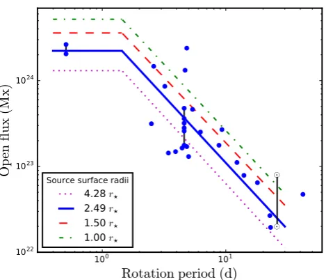
Figure 4. Open flux against rotation period calculated usingrss=2.49r (blue circles). Stars observed at multiple epochs are connected by a vertical line. A fit to these points is shown with a solid blue line. Fits to the open flux calculated usingrss=1.00r, 1.50rand 4.28rare also shown. The data
points for these fits are translated vertically in the plot when compared to therss=2.49rdata points and show a similar level of dispersion. However,
they are not plotted for clarity. The coefficients for these fits, as well as other fits using differentrssvalues, can be found in Table3. Two solar symbols
indicate the variation of the open flux over the solar cycle.
dipole components, we require a method of estimating the open flux as a function of rotation period and source surface radius. This is done as follows. First, we calculate the open flux of all the stars in our sample for a discrete set of different source surface radii,rss,i, in the range 1r–4.28r. Here,iis an index labelling the different source surface radii in this discrete set. For each of the source sur-face radii,rss,i, we perform a fit to the unsaturated stars, similarly to the one undertaken in Section 3.2, of the formopen,i=10ciProtmi, wheremiand ci are fit parameters. As in Section 3.2, the satu-rated value of the open flux is taken to be 10ciPmi
rot,crit. In Fig.4, we show the open flux values for one choice of the source surface radii,rss,i=2.49r(blue points) as well as the fit to these points
(solid blue line). This is the typical source surface radius chosen when studying the Sun. The PFSS model predicts solar open fluxes between∼2×10²²and∼8×10²²Mx (Jardine et al.2017). For a solar rotation period, we predict an open flux of 2.5×10²²Mx using our fit, in good agreement with the solar values. Additionally, we also show the fits for three other choices ofrss,ito illustrate the impact ofrss,ion the fits. The data points for these fits are not shown for clarity. A full list ofmiandcicoefficients for all values ofrss,i are available in Table3.
To calculate the open flux for an arbitraryProtandrss, we pick the tworss,ivalues from Table 3which bound our choice ofrss. Using themiandcivalues associated with these tworss,ivalues, we calculate two open flux values at the rotation period of interest, i.e. open,i=10ciProtmi. Lastly, we interpolate between these two
open,ivalues to determine the open flux for our chosenrss. When calculating the open flux using a rss > 4.28r, the dipolar term
strongly dominates (see Fig.3) and we simply use equation (7).
4 O P E N C L U S T E R DATA
In order to constrain our model, we use the rotation periods of stars in open clusters of known ages. Since we are studying rotation period evolution on the main sequence, we have chosen clusters that have ages of 125 Myr or greater. In recent years, rotation pe-riod measurements in clusters older than 1 Gyr have been possible thanks to theKepler Space Telescope(Meibom et al.2015; Barnes et al.2016). In particular, rotation period measurements from the 4 Gyr cluster M67 confirm that the Sun has a typical rotation period for a star of its age and mass (Barnes et al. 2016). The clusters we have used in this work and their ages are listed in Table4. For each cluster, we will consider all the stars with masses between 0.9 and 1.1 Mto be a representative of solar-mass stars. Fig.5
shows the distribution of rotation periods for these stars in each of the clusters as a function of age (plotted with grey plus symbols) as well as our rotational evolution tracks (these will be discussed in Section 5). We can see that the rotation period distributions evolve with time. At early ages (<200 Myr), solar-mass stars can have a large range of rotation periods with the fastest spinning nearly 100 times faster than the Sun. However, after∼1 Gyr, the rotation periods have nearly all converged on to a single valued track regard-less of their rotational history. Similar to previous studies (Gallet & Bouvier2013,2015; Johnstone et al.2015a), we will fit our model to the 25th, 50th and 90th percentiles of the rotation period distribu-tions in each cluster. Implicit in this method is the assumption that a star at a given percentile will remain at that percentile throughout its entire evolution. We use a boot strapping method to determine the rotation period at these percentiles for each cluster, as well as their errors. These are listed for each cluster in Table4. They are also plot-ted with red downwards triangles (25th percentile), green squares (50th percentile) and blue upwards triangles (90th percentile) in Fig.5.
5 T H E R OTAT I O N E VO L U T I O N O F A S O L A R - M A S S S TA R
[image:6.595.47.547.631.735.2]In this section, we will fit rotation evolution tracks to the 90th, 50th and 25th percentiles in each of the open clusters. We will refer to these as the fast, intermediate and slow tracks, respectively. In
Table 3. For a range of source surface radii,rss,i, we perform a fit of the formopen,i=10ciProtmito the unsaturated stars. Here, we list themiandcivalues for eachrss,i.
rss,i/r 1.00 1.30 1.50 1.69 1.88 2.10
mi −1.545±0.200 −1.522±0.206 −1.525±0.211 −1.533±0.215 −1.540±0.217 −1.547±0.219
ci 24.96±0.18 24.86±0.19 24.80±0.20 24.75±0.20 24.71±0.20 24.67±0.21
rss,i/r 2.27 2.49 2.67 2.89 3.07 3.29
mi −1.551±0.221 −1.554±0.222 −1.557±0.222 −1.559±0.223 −1.561±0.223 −1.563±0.224
ci 24.63±0.21 24.60±0.21 24.57±0.21 24.53±0.21 24.51±0.21 24.48±0.21
rss,i/r 3.41 3.55 3.70 3.87 4.07 4.28
mi −1.564±0.224 −1.565±0.224 −1.566±0.224 −1.566±0.224 −1.567±0.225 −1.568±0.225
Table 4. The open cluster data used in this study. For each cluster, we list the age as well as the 25th, 50th and 90th percentiles of the angular velocity distribution of∼solar-mass stars.
Cluster Age 25 50 90 Ref.
name (Myr) () () ()
Pleiades 125 4.83±0.14 6.14±0.24 44.91±9.63 Hartman et al. (2010) M50 130 4.39±0.46 5.45±0.34 23.01±8.67 Irwin et al. (2009) M35 150 4.39±0.10 5.12±0.23 24.90±4.90 Meibom, Mathieu & Stassun (2009) M34 220 3.77±0.17 4.75±0.63 28.89±4.74 Meibom et al. (2011b) M37 550 3.08±0.04 3.34±0.03 4.46±0.67 Hartman et al. (2009) Praesepe 580 2.64±0.05 2.76±0.04 2.85±0.03 Delorme et al. (2011) Hyades 625 2.68±0.07 2.75±0.06 3.07±0.05 Delorme et al. (2011) NGC 6811 1000 2.32±0.02 2.42±0.02 2.59±0.05 Meibom et al. (2011a) NGC6819 2500 1.20±0.01 1.22±0.01 1.39±0.05 Meibom et al. (2015) M67 4200 0.83±0.02 0.92±0.03 1.04±0.03 Barnes et al. (2016)
Figure 5. The rotation evolution of a solar-mass star. Plus symbols indicate the observed rotation periods of solar-mass stars in open clusters. Blue upwards triangles, green squares and red downwards triangles represent the 90th, 50th and 25th percentile in each of the clusters, respectively. The blue, green and red tracks show the rotation evolution of a fast, intermediate and slow solar-mass star as calculated with the dipole method (solid lines) and the multipolar method (dashed lines). The horizontal dashed line indicates the saturation threshold. Data and references for the cluster data can be found in Table4.
order to determine the best-fitting values for the power-law index of the source surface radii scaling,n, and the scaling constant used to determine the spin-down torque,k, we require a goodness-of-fit parameter. We will use
X=
j
(logobs,j−logmodel,j)2. (9)
Here, obs,j refers to the observed angular velocities from open clusters andmodel,jrefers our model’s estimate ofobs,j. The sum-mation over the index,j, is performed over the 25th, 50th and 90th percentiles for every cluster as shown in Table4. This is a similar goodness-of-fit parameter to that used by Johnstone et al. (2015a). However, unlike these authors, we do not assign different weights to the different clusters. Tests indicate that giving older clusters a larger weighting does not significantly change our results.
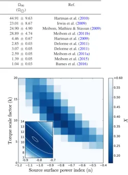
In Fig.6, we calculate the value ofXover a grid ofnandkvalues using the dipole method of determining the open flux (as described in Section 3.2). There is a well-defined minimum inXwhich occurs
Figure 6. The goodness-of-fit parameter,X, calculated over a grid of source surface power indices,n, and torque scalefactors,k, for the dipolar method. Xvalues larger than 0.6 have been truncated to 0.6. The inset shows a higher resolution search through thenandkvalues around the minima. Contours forX={0.16, 0.19, 0.3}are also shown on the inset. The minimum inX occurs atndip= −0.84 andkdip=10.64.
atndip = −0.84 and kdip = 10.64. It is worth noting that some degeneracy exists between ndip and kdip however. A more (less) negative value ofndipcan be partially offset by a larger (smaller)
kdipvalue for only a small increase in our goodness-of-fit parameter. Usingndip andkdip, we calculate the fast, intermediate and slow tracks that are plotted with solid red, green and blue lines in Fig.5. By combining equations (7) and (8) with the fit from Fig.2and the value ofndip, we can also determine the functional dependence of the open flux on the rotation period in our model. This is given by
open,dip=7.27×10²³
˜
P−3.26 rot 31.3 ˜Prot−2.52+1
, (Prot> Prot,crit)
open,dip,sat =2.00×10²³, (Prot< Prot,crit), (10)
where ˜Prot=Prot/Prot,.
[image:7.595.293.545.82.426.2](Pantolmos & Matt2017). Additionally, the mass-loss rates we use may be systematically underestimated causing a lower than ex-pected spin-down torque. It is worth emphasizing that mass-loss rates are extremely difficult to estimate and poorly constrained ob-servationally. Differences between the mass-loss rate estimated by the model of Cranmer & Saar (2011) and the real mass-loss rates of stars could be absorbed into the fit parameterk(and perhapsn). Currently, there is no way of determining how much of the fact thatkdipis larger than 1 can be attributed to inaccurately estimat-ing mass-loss rates. Although the mass-loss rates predicted by the model of Cranmer & Saar (2011) agree reasonably well with obser-vations of the Sun, they may be less accurate for younger or more rapidly rotating stars. Lastly, we have assumed solid body rotation for simplicity. However, if core-envelope decoupling were included, the stellar wind braking should be more efficient since it would be acting on the envelope only. This should reduce the value ofkdip which we obtain with our model. Johnstone et al. (2015a) obtain a torque scaling value of 11 within their model which is comparable to our value. However, Gallet & Bouvier (2015) obtained a value of 1.7 in their solar-mass models which suggests their models may be capturing the relevant physics more accurately.
It is also worth noting that the particular values ofndipandkdipwe obtain are dependent on the form of the flux–rotation relation that we adopt, i.e. the fit from Fig.2. For example, if we only fit to the stars in Fig.2with masses 0.95 M ≤M≤1.05 M, we recover
ndip= −0.67 andkdip=8.25. It is clear that more ZDI observations of solar-mass mass stars are needed in order to refine our model. For the remainder of this work, we will consider the canonicalndipand
kdipvalues to be those determined using the full ZDI sample, i.e. the stars with masses 0.9 M ≤M≤1.1 Msince this matches the mass bin width chosen for the open cluster rotation period data. We perform this procedure again but using the multipolar method to determine the open flux (as described in Section 3.3). The equiv-alent plot of Fig.6for the multipolar method looks very similar (not shown) with a minimum inXoccurring atnmulti= −0.82 and
kmulti=10.18. These values are similar to those calculated using the dipole-only method. Using the multipolar method of determining the open flux in conjunction with thenmultiandkmultivalues, we plot the fast, intermediate and slow rotator tracks in Fig.5with dashed lines. The dashed rotation tracks lay almost exactly on the top of the solid rotation tracks determined using the dipolar method.
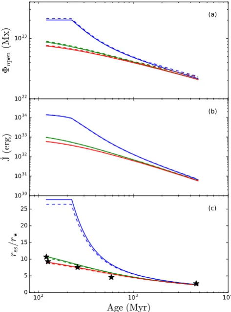
In Figs7a and7b, we plot the open flux and angular momentum-loss rate for both the dipolar and multipolar methods. The open flux and angular momentum-loss rates are both monotonically de-creasing functions of age for the fast, intermediate and slow tracks. However, the fast tracks show a change in behaviour at∼200 Myr. As can be seen in Fig.5, this is the age at which fast track stars tran-sition from the saturated to the unsaturated regime. Unlike the fast track, stars on the intermediate and slow tracks are never rotating quickly enough to be in the saturated regime.
[image:8.595.309.546.57.376.2]To understand why the two methods produce such similar results, we need to understand how the source surface radius evolves over the main sequence. Fig.7c shows the source surface radius evolution for the fast, intermediate and slow tracks. These are calculated using equation (8) in conjunction with the rotation evolution tracks shown in Fig.5and our best-fitting values forndipandnmulti. Over the course of the main sequence, the source surface radii of these stars shrink as the star spins down and magnetic activity declines. For the intermediate and slow rotators, the source surface radius steadily drops from∼10rat∼100 Myr to∼2.5rby the age of the Sun. However, the fast rotator is spinning rapidly enough during its early main-sequence lifetime that its source surface radius attains
Figure 7. (a) Open flux, (b) angular momentum-loss rate and (c) source surface radii against age. In each panel, tracks are shown for fast (blue), intermediate (green) and slow (red) rotators calculated using the dipolar (solid lines) and multipolar (dashed lines) methods. In panel (c), the optimal source surface radii for a number of roughly solar-mass stars, as determined by R´eville et al. (2016), are shown with star symbols (see the text). the saturation value of∼25r. Indeed, no solar-mass star can have a source surface radius larger than the saturation value under this model. From Fig.3and Table2, we see that, for the majority of the stars in our sample, large differences in the open flux obtained from the dipolar and multipolar methods only occur at source surface radii smaller than roughly two or three stellar radii. Since all three tracks (and the tracks for any other percentile one might calculate) maintain source surface radii larger than 2.5runtil the age of the Sun, it should be a no surprise that there is very little difference between the dipolar and multipolar methods for calculating the open flux in the range of ages we have studied here. If we were to extend the rotation tracks to ages significantly past the age of the Sun, it is possible that the source surface radii would become small enough for the differences between the two methods of calculating the open flux to matter. However, currently, the rotation period behaviour of stars much older than the Sun is unclear. We will discuss this issue further in Section 6.
each star. They then modelled each star with a PFSS model and determined the source surface radius that would be required for the PFSS model to produce the same open flux as their MHD models. These optimum source surface radii are plotted in Fig. 7c with star symbols. We can compare the optimum source surface radii of R´eville et al. (2016) to the source surface radii as estimated by our own model. Takingnmulti= −0.82 from our multipolar method, we predict source surface radii of 13.5r, 10.1r, 16.4r, 9.0rand 6.3r for BD-16351, TYC 5164-567-1, HII 296, DX Leo and AV 2177, respectively. The optimum source surface radii that R´eville et al. (2016) predict are 8.1r, 10.7r, 9.3r, 7.6r and 4.6r. We see that our estimates are close to those of R´eville et al. (2016) but our model tends to produce source surface radii that are larger, sometimes by a factor of∼1.7. It is worth pointing out that the stars modelled by R´eville et al. (2016) are all slow/moderate rotators. Our model predicts that the source surface radii of slowly/moderately rotating stars only change by a factor of a few. A similar study to that of R´eville et al. (2016) modelling stars on the rapidly rotating track, where the source surface radii appear to change much more drastically over the main sequence in our model, would provide a much more stringent comparison.
Lastly, it is worth commenting on the source surface radii values. Our model estimates that the fastest rotators haverss>25rwhich
is an order of magnitude larger than the Sun’s source surface radii. Our simplified model requires that the source surface radii be this large for the fastest rotators but it is not clear whether, in reality, closed field loops can be maintained out to such a large distance. For instance, magnetocentrifugal forces acting on the coronal plasma may cause closed loops to open up closer to the stellar surface than they otherwise would have. Since our model does not self-consistently model the interactions between the stellar wind plasma and magnetic field, it is not possible to say how large an effect this might have. Such questions are left to future investigations and will require more sophisticated modelling of the relevant physics to answer.
6 D I S C U S S I O N A N D C O N C L U S I O N S
In this work, we have used a PFSS model, in conjunction with a sample of ZDI maps, to analyse how the open flux of solar-mass stars varies as a function of rotation and source surface radius. We then use these open flux relationships and the braking law of R´eville et al. (2015a) to model the rotation period evolution of solar-mass stars on the main sequence up to the age of the Sun. We have assumed solid body rotation for simplicity. Within the PFSS model, the source surface radius is a free parameter. Previous works using this model have typically set the source surface radius to a value close to the solar value (∼2.5r). However, in this work, using rotation period data from open clusters, we are able to constrain how the source surface radius varies with the rotation period of the star. We predict that the fastest rotators begin life on the main sequence with a source surface radius of∼26r while the intermediate and slower rotators start out with a source surface radius of∼10r. Eventually, the source surface radii of solar-mass stars will converge and reach the solar source surface radius by the age of the Sun.
Previous rotation period evolution models have typically used braking laws that are formulated in terms of the dipolar surface magnetic field strength (e.g. Matt et al.2012b). However, we use the braking law of R´eville et al. (2015a), which is formulated in terms of the open flux. In principle, this braking law allows us to account for higher order spherical harmonic modes in the surface magnetic
field. In practice, however, we find that the dipole component of the magnetic field dominates the open flux for all but the smallest choices of the source surface radius. As outlined in Section 5, the dipolar open flux in our model can be analytically calculated as a function of rotation period by combining equations (7) and (8) with the fit from Fig.2.
When considering the effect of field geometry on angular mo-mentum evolution, our results suggest that it would be reasonable to use the braking law of Matt et al. (2012b) over that of R´eville et al. (2015a). However, some caution should be exercised when directly comparing models using the two braking laws. The model we have presented uses two fit parameters. These are the power-law indices for the source surface radius,n, and the torque scaling parameter,k. Other models that use the braking law of Matt et al. (2012b) usually have a similar torque scaling parameter to the one used in this work. However, since they do not have to model the open flux, they do not need a fit parameter like ourn. Instead, these models have other free parameters. For instance, disc lifetimes are a free parameter in the work of Gallet & Bouvier (2013) and Gallet & Bouvier (2015) while the mass-loss rates used by Johnstone et al. (2015a) are specified as power laws of mass and rotation, where the power-law indices are fit parameters. Uncertainties in different models are therefore absorbed in different places making a direct comparison between models difficult. In the future, these uncertainties can be reduced through further observations of the rotation period distributions of open clusters, magnetic field strengths and disc lifetimes.
For this work, we have restricted ourselves to studying solar-mass stars on the main sequence up the age of Sun. However, this is only one part of the lifetime of a star. In comparison to the main sequence, modelling the rotation period evolution of stars on the PMS is much more difficult. Early on, in the classical T Tauri phase, the presence of a circumstellar disc is an additional element that must be con-sidered. Throughout the entire PMS stars spin-up as they contract towards the main sequence. However, their rotational velocities are much slower than expected from contraction alone (Vogel & Kuhi1981) indicating that significant spin-down torques are acting on PMS stars. There is strong evidence that the presence of discs inhibits the spin-up of these stars (Edwards et al.1993; Bouvier, Forestini & Allain1997; Rebull, Wolff & Strom2004) although the precise mechanism by which this is achieved is still unclear. Common suggestions include disc locking (Choi & Herbst1996) or accretion-powered stellar winds (Matt et al.2010,2012a). Ad-ditionally, changes in the surface magnetic field associated with internal structure changes may also play a role (Gregory et al.2012; Folsom et al.2016).
In contrast to young main-sequence stars, the rotation period evolution of stars older than the age of the Sun remains relatively unconstrained. Consequently, rotation evolution models, such as the one we have presented, cannot be extended beyond the age of the Sun with any reliability. However, recent advances have allowed for the determination of rotation periods and asteroseismic ages of old field stars (Garc´ıa et al. 2014). These stars appear to be rotating much faster than expected from gyrochronology. Indeed, dramatically reduced braking appears to be required to explain the rapid rotation of these stars (van Saders et al.2016). One possible explanation for such a reduction is that the nature of the dynamo changes at a Rossby number of∼2 such that the surface magnetic field is concentrated into smaller scales (Metcalfe, Egeland & van Saders2016). Under this interpretation, the Sun (Rossby number
the dipole component of the magnetic field which predominantly governs the rotation evolution of main-sequence solar-mass stars, to break down at old ages. This suggestion will take time to confirm, however, since there are currently no ZDI observations of stars with Rossby numbers much bigger than 2.
In principle, the technique we have outlined in this work can also be applied to stars of other masses. However, there would be a number of additional barriers to overcome. First, more ZDI maps of saturated stars would be required. Presently, the open flux behaviour for solar-type stars in the saturated regime is relatively unconstrained in comparison to the unsaturated regime (see fig. 2b of See et al.2017). As discussed in Section 5, for solar-mass stars, only the most rapid rotators spend any time in the saturated regime and those that do, rapidly spin-down into the unsaturated regime. Therefore, the loose constraints on the saturated level of the open flux for solar-mass stars are not a large problem. However, the crit-ical rotation period at which saturation sets in increases for lower mass stars. This is easily seen in fig. 6 of Johnstone et al. (2015a). Consequently, the loose constraints in the saturated regime are more problematic for lower mass stars since they can spend more time in the saturated regime. Secondly, the method we have used to esti-mate our source surface radii is calibrated to the Sun (equation 8). Since the source surface radii of other stars are unknown, we would have nothing to calibrate to when studying the angular momentum evolution of stars with different masses. A possible method of over-coming this problem would be to recast equation (8) asrss=αProtn, whereαis a constant of proportionality. This would, however, in-troduce another parameter to fit for. Finally, the magnetic properties of the very lowest masses (<0.2 M) appear to exist in one of the two states: either strong and dipolar or weak and multipolar (Morin et al.2010). See et al. (2017) showed that the spin-down properties corresponding to these two states are very different with the instan-taneous spin-down time-scales of the strong dipolar stars being two orders of magnitude shorter than their weak multipolar counter-parts. As discussed by these authors, detailed angular momentum evolution modelling of these stars must wait until the number of
<0.2 Mstars of known ages which have been mapped with ZDI is vastly expanded.
AC K N OW L E D G E M E N T S
The authors thank an anonymous referee who helped improve the quality of this manuscript as well as Isobelle Baraffe, Sean Matt and Florian Gallet for useful discussions regarding this work. VS acknowledges support from a Science & Technology Facilities Council (STFC) post-doctoral fellowship and the European Re-search Council Consolidator grant AWESoMeStars. SBS and SVJ acknowledge research funding by the Deutsche Forchungsgemein-schaft (DFG) under grant SFB, project A16. RF acknowledges fi-nancial support by WOW from INAF through the Progetti Premiali funding scheme of the Italian Ministry of Education, University, and Research. This study was supported by the grant ANR 2011 Blanc SIMI5-6 020 01 ‘Toupies: Towards understanding the spin evolution of stars’ (http://ipag.osug.fr/Anr_Toupies/). This work is based on observations obtained with ESPaDOnS at the CFHT and with NARVAL at the TBL. CFHT/ESPaDOnS are operated by the National Research Council of Canada, the Institut National des Sciences de l’Univers of the Centre National de la Recherche Sci-entifique (INSU/CNRS) of France and the University of Hawaii, while TBL/NARVAL are operated by INSU/CNRS. We thank the CFHT and TBL staff for their help during the observations.
R E F E R E N C E S
Altschuler M. D., Newkirk G., 1969, Sol. Phys., 9, 131
Amard L., Palacios A., Charbonnel C., Gallet F., Bouvier J., 2016, A&A, 587, A105
Baraffe I., Homeier D., Allard F., Chabrier G., 2015, A&A, 577, A42 Barnes S. A., 2003, ApJ, 586, 464
Barnes S. A., 2007, ApJ, 669, 1167 Barnes S. A., 2010, ApJ, 722, 222
Barnes S. A., Weingrill J., Fritzewski D., Strassmeier K. G., Platais I., 2016, ApJ, 823, 16
Blackman E. G., Owen J. E., 2016, MNRAS, 458, 1548
Boro S. S., Jeffers S. V., Petit P., Marsden S., Morin J., Folsom C. P., 2015, A&A, 573, A17
Boro S. S. et al., 2016, A&A, 594, A29
Bouvier J., Forestini M., Allain S., 1997, A&A, 326, 1023 Brown T. M., 2014, ApJ, 789, 101
Brown S. F., Donati J.-F., Rees D. E., Semel M., 1991, A&A, 250, 463 Choi P. I., Herbst W., 1996, AJ, 111, 283
Cohen O., Drake J. J., 2014, ApJ, 783, 55 Cranmer S. R., Saar S. H., 2011, ApJ, 741, 54
Delorme P., Collier C. A., Hebb L., Rostron J., Lister T. A., Norton A. J., Pollacco D., West R. G., 2011, MNRAS, 413, 2218
do Nascimento J.-D., Jr, et al., 2016, ApJ, 820, L15 Donati J.-F., Brown S. F., 1997, A&A, 326, 1135 Donati J.-F. et al., 2003a, MNRAS, 345, 1145
Donati J.-F., Collier C. A., Petit P., 2003b, MNRAS, 345, 1187 Donati J.-F. et al., 2006, MNRAS, 370, 629
Edwards S. et al., 1993, AJ, 106, 372 Fares R. et al., 2010, MNRAS, 406, 409
Fares R., Moutou C., Donati J.-F., Catala C., Shkolnik E. L., Jardine M. M., Cameron A. C., Deleuil M., 2013, MNRAS, 435, 1451
Folsom C. P. et al., 2016, MNRAS, 457, 580 Gallet F., Bouvier J., 2013, A&A, 556, A36 Gallet F., Bouvier J., 2015, A&A, 577, A98
Gallet F., Charbonnel C., Amard L., Brun S., Palacios A., Mathis S., 2017, A&A, 597, A14
Garc´ıa R. A. et al., 2014, A&A, 572, A34
Garraffo C., Drake J. J., Cohen O., 2015, ApJ, 807, L6
Gregory S. G., Jardine M., Collier C. A., Donati J.-F., 2006, MNRAS, 373, 827
Gregory S. G., Donati J.-F., Morin J., Hussain G. A. J., Mayne N. J., Hillenbrand L. A., Jardine M., 2012, ApJ, 755, 97
Guirado J. C. et al., 2010, Astrophys. Space Sci. Proc., 14, 139 Hartman J. D. et al., 2009, ApJ, 691, 342
Hartman J. D., Bakos G. ´A., Kov´acs G., Noyes R. W., 2010, MNRAS, 408, 475
Irwin J., Aigrain S., Bouvier J., Hebb L., Hodgkin S., Irwin M., Moraux E., 2009, MNRAS, 392, 1456
Isobe T., Feigelson E. D., Akritas M. G., Babu G. J., 1990, ApJ, 364, 104
Jardine M., Collier C. A., Donati J.-F., 2002, MNRAS, 333, 339 Jardine M., Vidotto A. A., See V., 2017, MNRAS, 465, L25
Jeffers S. V., Petit P., Marsden S. C., Morin J., Donati J.-F., Folsom C. P., 2014, A&A, 569, A79
Johnstone C. P., Jardine M., Gregory S. G., Donati J.-F., Hussain G., 2014, MNRAS, 437, 3202
Johnstone C. P., G¨udel M., Brott I., L¨uftinger T., 2015a, A&A, 577, A28 Johnstone C. P. et al., 2015b, ApJ, 815, L12
Lammer H., Selsis F., Ribas I., Guinan E. F., Bauer S. J., Weiss W. W., 2003, ApJ, 598, L121
Lang P., Jardine M., Donati J.-F., Morin J., Vidotto A., 2012, MNRAS, 424, 1077
Lang P., Jardine M., Morin J., Donati J.-F., Jeffers S., Vidotto A. A., Fares R., 2014, MNRAS, 439, 2122
Mamajek E. E., Hillenbrand L. A., 2008, ApJ, 687, 1264
Matt S. P., MacGregor K. B., Pinsonneault M. H., Greene T. P., 2012b, ApJ, 754, L26
Matt S. P., Brun A. S., Baraffe I., Bouvier J., Chabrier G., 2015, ApJ, 799, L23
Meibom S., Mathieu R. D., Stassun K. G., 2009, ApJ, 695, 679 Meibom S. et al., 2011a, ApJ, 733, L9
Meibom S., Mathieu R. D., Stassun K. G., Liebesny P., Saar S. H., 2011b, ApJ, 733, 115
Meibom S., Barnes S. A., Platais I., Gilliland R. L., Latham D. W., Mathieu R. D., 2015, Nature, 517, 589
Mestel L., Spruit H. C., 1987, MNRAS, 226, 57
Metcalfe T. S., Egeland R., van Saders J., 2016, ApJ, 826, L2
Morin J., Donati J.-F., Petit P., Delfosse X., Forveille T., Jardine M. M., 2010, MNRAS, 407, 2269
Nicholson B. A. et al., 2016, MNRAS, 459, 1907
Noyes R. W., Hartmann L. W., Baliunas S. L., Duncan D. K., Vaughan A. H., 1984, ApJ, 279, 763
Pantolmos G., Matt S. P., 2017, ApJ, 849, 83 Petit P. et al., 2008, MNRAS, 388, 80
Pizzolato N., Maggio A., Micela G., Sciortino S., Ventura P., 2003, A&A, 397, 147
Rebull L. M., Wolff S. C., Strom S. E., 2004, AJ, 127, 1029 Reiners A., Mohanty S., 2012, ApJ, 746, 43
R´eville V., Brun A. S., Matt S. P., Strugarek A., Pinto R. F., 2015a, ApJ, 798, 116
R´eville V., Brun A. S., Strugarek A., Matt S. P., Bouvier J., Folsom C. P., Petit P., 2015b, ApJ, 814, 99
R´eville V., Folsom C. P., Strugarek A., Brun A. S., 2016, ApJ, 832, 145 Ribas I. et al., 2016, A&A, 596, A111
See V., Jardine M., Vidotto A. A., Petit P., Marsden S. C., Jeffers S. V., do Nascimento J. D., 2014, A&A, 570, A99
See V., Jardine M., Fares R., Donati J.-F., Moutou C., 2015a, MNRAS, 450, 4323
See V. et al., 2015b, MNRAS, 453, 4301 See V. et al., 2016, MNRAS, 462, 4442 See V. et al., 2017, MNRAS, 466, 1542 Semel M., 1989, A&A, 225, 456
Tu L., Johnstone C. P., G¨udel M., Lammer H., 2015, A&A, 577, L3 van Saders J. L., Ceillier T., Metcalfe T. S., Silva A. V., Pinsonneault M. H.,
Garc´ıa R. A., Mathur S., Davies G. R., 2016, Nature, 529, 181 Vidotto A. A., Jardine M., Morin J., Donati J.-F., Lang P., Russell A. J. B.,
2013, A&A, 557, A67
Vidotto A. A., Jardine M., Morin J., Donati J. F., Opher M., Gombosi T. I., 2014a, MNRAS, 438, 1162
Vidotto A. A. et al., 2014b, MNRAS, 441, 2361 Vogel S. N., Kuhi L. V., 1981, ApJ, 245, 960
Wood B. E., M¨uller H.-R., Redfield S., Edelman E., 2014, ApJ, 781, L33 Wright N. J., Drake J. J., Mamajek E. E., Henry G. W., 2011, ApJ, 743, 48
A P P E N D I X A : D E R I V I N G T H E D I P O L A R O P E N F L U X
In this appendix, we derive the ratio of open flux to surface flux for a pure dipole mode. We remind the reader that the radial component of the magnetic field,Br, in the PFSS model is given by
Br= −
N
l=1
l
m=−l
[lalmrl−1−(l+1)blmr−(l+2)]Plm(cosθ) eimφ.
(A1)
From equations (4) and (5), the condition thatBθ(rss)=Bφ(rss)=0 requires that thealmandblmcoefficients obey the relation
almrssl−1+blmr− (l+2)
ss =0. (A2)
Combining equations (A1) and (A2), one finds that
Br=
N
l=1
l
m=−l
Blmfl(r)Plmeimφ, (A3)
whereBlmandfl(r) are given by
Blm= −almlrl−1+blm(l+1)r−(l+2), (A4)
fl(r)=
(l+1)˜r−(l+2)+lr˜−(2l+1) ss r˜l−1
lr˜ss−(2l+1)+(l+1)
, (A5)
where ˜r=r/rand ˜rss=rss/r. For a dipole, equation (A3)
there-fore reduces to
Br=B10f1(r) cosθ, (A6)
where we have chosen to use thel=1,m=0 mode and note that the Legendre polynomialP10is given by cosθ. An identical result is obtained for thel=1,m=1 mode or any combination of the
l=1 modes but we will proceed with thel=1,m=0 mode for convenience. In equation (A6),f1(r) is given by
f1(r)= 2˜r
−3+r˜−3 ss ˜
r−3 ss +2
. (A7)
The flux at a given radial distance from the stellar surface for a pure dipole mode is therefore given by
10(r)=
—
S|B
r(r)|dS
=B10f1(r)r2
|cosθ|sinθdθ
dφ
=2πB10f1(r)r2, (A8)
whereSis a spherical surface of radiusr. Finally, the ratio of the open flux to the surface flux for a pure dipole mode is given by
10(rss)
10(r) =
f1(rss)
f1(r)
rss
r
2
. (A9)
Substituting equation (A7), one obtains
10(rss)
10(r) =
open,dip
,dip
= 3˜rss2 2˜r3
ss+1
. (A10)