On the Index of Repeatability: Estimation and Sample Size Requirements

ISSN Online: 2161-7198 ISSN Print: 2161-718X

DOI: 10.4236/ojs.2019.94035 Aug. 20, 2019 530 Open Journal of Statistics

On the Index of Repeatability:

Estimation and Sample Size Requirements

Maha Al-Eid

1

, Mohamed M. Shoukri

2*

1_{Department of Biostatistics, Epidemiology and Scientific Computing, King Faisal Specialist Hospital and Research Center,} Riyadh, KSA

2_{Department of Epidemiology and Biostatistics, Schulich School of Medicine and Dentistry, London, Ontario, Canada}

Abstract

Background: Repeatability is a statement on the magnitude of measurement error. When biomarkers are used for disease diagnoses, they should be meas-ured accurately. Objectives: We derive an index of repeatability based on the ratio of two variance components. Estimation of the index is derived from the one-way Analysis of Variance table based on the one-way random effects model. We estimate the large sample variance of the estimator and assess its adequacy using bootstrap methods. An important requirement for valid esti-mation of repeatability is the availability of multiple observations on each subject taken by the same rater and under the same conditions. Methods: We use the delta method to derive the large sample variance of the estimate of repeatability index. The question related to the number of required repeats per subjects is answered by two methods. In first methods we estimate the number of repeats that minimizes the variance of the estimated repeatability index, and the second determine the number of repeats needed under cost-constraints. Results and Novel Contribution: The situation when the measurements do not follow Gaussian distribution will be dealt with. It is shown that the required sample size is quite sensitive to the relative cost. We illustrate the methodologies on the Serum Alanine-aminotransferase (ALT) available from hospital registry data for samples of males and females. Re-peatability is higher among females in comparison to males.

Keywords

Measurements Errors, Functions of Variance Components, Delta Method, Lagrange Multiplier, Bootstrap Technique

1. Introduction

Repeatability and reproducibility are ways of measuring precision, particularly How to cite this paper: Al-Eid, M. and

Shoukri, M.M. (2019) On the Index of Repeatability: Estimation and Sample Size Requirements. Open Journal of Statistics, 9, 530-541.

https://doi.org/10.4236/ojs.2019.94035 Received: July 30, 2019

Accepted: August 17, 2019 Published: August 20, 2019

Copyright © 2019 by author(s) and Scientific Research Publishing Inc. This work is licensed under the Creative Commons Attribution International License (CC BY 4.0).

http://creativecommons.org/licenses/by/4.0/

DOI: 10.4236/ojs.2019.94035 531 Open Journal of Statistics in the fields of biochemistry, radiology, and medical diagnoses. In general, scien-tists perform the same experiment several times in order to confirm their find-ings. These findings may show variations. In the context of an experiment, re-peatability measures the variation in measurements taken by a single instrument or person under the same conditions, while reproducibility measures whether an entire study or an experiment can be reproduced. There has been confusion in the literature about the way that repeatability and reproducibility are quantified. Both concepts were often reported as either standard deviations or coefficient of variations.

The main focus of this paper is on the concept of repeatability, which was first introduced by Bland and Altman [1]. For repeatability to be established, the fol-lowing conditions must be in place: the measurements should be taken in the same location; the same measurement procedure; the same observer; the same measuring instrument, used under the same conditions; and repetition over a short period of time.

What’s known as “the repeatability” is in fact a measurement of precision, which denotes the absolute difference between a pair of repeated test results. We note that when we have more than two readings per subject the idea of pairing produces several repeatability coefficients and the concept becomes unclear.

Repeatability is also known as test-retest reliability indicating the closeness of the agreement between the results of successive measurements of the same mea-surand carried out under the same conditions of measurement. A less-than-perfect test-retest reliability causes test-retest variability. Such variabil-ity can be caused by, for example, intra-individual variabilvariabil-ity and intra-observer variability. A measurement may be said to be repeatable when this variation is smaller than a pre-determined acceptance criterion. A complete account on the reliability literature can be found in Shoukri [2] [3].

One of the most important applications of the concept of repeatability is in the construction of the normal range or reference range in clinical medicine, which relies on the availability of a large sample of healthy individuals. Research has shown that the distribution of these measurements is affected by two main sources of variations: the between subjects and the within subject-components of variations.

This paper has three-fold objectives: Firstly; we define a proposed index of repeatability, as the ratio of the within-subjects’ variations to the between subject variation. The within subject variation is expected to be quite small relative to the between subjects-variations. To formalize the presentation, we assume that a single measurement yi from subject i=1,2, , k is written as:

i i i

y = + +µ s e ₍₁₎ Hence si represents the sources of between-subjects biological variation, and i

addi-DOI: 10.4236/ojs.2019.94035 532 Open Journal of Statistics tive under the logarithmic transformation. Following Harries and De Mets [4] it is further assumed that _~

(

_0, 2

)

i s

s N

σ

_{, and ~}

(

_0, 2

)

i e

e N

σ

_{and that} s_i ⊥e_{i for} all i. We define the “Repeatability Index Parameter” (RIP) as 2 2

e s θ σ σ= _.

The salient point is that

θ

_{cannot be estimated unless we have at least two}

repeated measurements on any subject in the study.

In Section 2 we specify the model generating the observations and discuss a general method of estimating RIP from a sample of k subjects when there is an opportunity to have n repeated samples per subject. In Section 3, we provide two alternatives for the sampling strategies. The first, we assume that the investigator has decided to acquire on total number of measurements N kn= _{, and the}

question becomes; what is the best split between

( )

k n, , that maximizes the ac-curacy of estimating RIP?

One of the biggest obstacles in clinical studies is the cost constraints. There-fore, the second strategy is to find the optimal split of N kn= _{, so that IRP is}

es-timated with maximum precision under cost restrictions (constrained optimiza-tion). The third objective of the study is to address the issue of estimating RIP when the assumption of the Gaussian distribution of observation is not tenable.

2. Model Specifications and Parameter Estimation

We assume that for subject i,n replicates of the same variable of interest yij are taken by the same instrument at the same time, so that

ij i ij

y = + +µ s e (2)

1,2, ,

i=  k

k is the number of subjects

1,2, ,

j= n

n is the number of replications per subject

We further assume that the components of the model described by (2) are such that:

(

2

)

~ 0,

i s

s N

σ

_{, are independently distributed random variables measuring the}

subjects effect, are independently distributed of the within subjects variation denoted by _~

(

_0, 2

)

ij e

e N

σ

_.

Under the additivity assumption of the model components, we have:

( )

2 2 2

(

2 2

)

2

(

)

var yij =

σ

s +

σ

e =

σ

s 1+

σ σ

e s =

σ

s 1+

θ

The parameter 2 2 e s

θ σ σ= _{is the target parameter of interest, named}

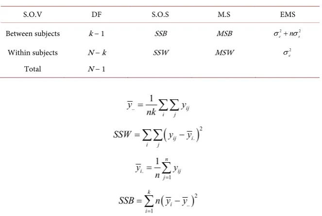
“Re-peatability Index Parameter” (RIP). The components of variation of the model set-up can be estimated using the well-known one-way Analysis of Variance (ANOVA) with random effects (Table 1).

[image:4.595.209.541.83.306.2]

DOI: 10.4236/ojs.2019.94035 533 Open Journal of Statistics

Table 1. The ANOVA set-up.

S.O.V DF S.O.S M.S EMS

Between subjects k − 1 SSB MSB 2 2

e n s

σ + σ

Within subjects N − k SSW MSW 2

e

σ

Total N − 1

.. 1 ij i j y y nk =

∑∑

(

)

2

. ij i i j

SSW =

∑∑

y −y

. 1 1 n i ij j y y n = =

∑

(

)

2

.. 1

k i i

SSB n y y

=

=

∑

−

The moment estimator of the parameter

θ

_{, and hence the maximum}

like-lihood estimator (under balanced design) is given by:

ˆ _n MSW

MSB MSW

θ

_{= } _

−

  (3) The parameter estimator θˆ given in Equation (3) is a nonlinear function of the sample statistics, and therefore an exact expression for its variance is not available. We use the delta method (Kendall and Stuart, 1989) [5], to obtain the first approximation of the variance of θˆ given by:

( )

(

)

(

)

(

)

2

2

ˆ

var var 2cov ,

var

MSB MSB MSW

MSB MSB MSW

MSW

MSW

θ θ θ

θ θ  ∂   ∂  ∂  = _{ } + _{  } ∂ ∂ ∂       ∂  + _{ } ∂     

 (4)

Substituting the required quantities in (4) and simplifying we get the first or-der approximation of the variance of θˆ as:

( )

₍

2

(

₎₍

)

2

₎

8

2 ˆ var 1 1 n v N n θ θ θ θ + = =

− + (5)

An

(

1−α

)

100% _{approximate Wald’s confidence interval on}

θ

may be constructed as:

ˆ _{z v}

θ ± ₍₆₎ where z in Equation (6) is the

(

1−α 2 100%

)

_{cut-off point from the standard}

normal table.

3. How Many Repeats Do We Need?

DOI: 10.4236/ojs.2019.94035 534 Open Journal of Statistics that N kn= _{is fixed a priori, and one needs to determine the number of}

repli-cates that minimizes the variance v, as given in (5).

Minimizing v with respect to the number of replications per subjects and solving for n we get:

0 2

v _n

n θ

∂ _{= ⇒ = +}

∂ (7)

(

)

2

2 1 2 0

2 1

v

n θ

∂ _{= >}

∂ +

This means that var

( )

θ

ˆ is minimized (i.e. maximizing precision) when at least 2 repeats are attained from each subject as shown in Equation (7). When

0

θ

= (no within subject-variation) then n=2 precisely.

We may also estimate the number of repeats for fixed width confidence inter-val as follows:

Suppose that we have decided on the number of subjects k. The question now is how many repeats per-subject are needed to estimate

θ

_{with 95% confidence}

such that the width of the confidence interval has a maximum given length w. Since the length of the Wald’s confidence interval is given as:

(

)

( )

ˆ 2 1.96 var

w= θ

(

)

(

)

(

) (

)

2 2 2

2

8

4 1.96 2

1 1 n w kn n θ θ θ ⋅ + = + −

Let

(

)

(

)

8 2 2 2 1 1 8 1.96 kw A θ θ + = >

Solving for n we have:

(

)

(

)

(

)

1 2 2

2 4 4

2 1

A A A

n

A

θ  θ θ 

+ +_ + + _

=

− (8)

This closed form expression is quite simple, and the computation of n from Equation (8), is straight forward. Substituting

θ

=0.25_, k=100_{, and} w=1 _in

(8), then n=156.

DOI: 10.4236/ojs.2019.94035 535 Open Journal of Statistics primarily on the size of the sample, and includes the data collection costs, sub-jects recruiting costs, management and technicians’ costs. On the other hand, overhead costs remain fixed regardless of the sample size. The total cost is as-sumed this additive formula

0 1 2

T t= +kt nkt+ (9) In Equation (9) t0 is the fixed cost, t1 is the cost of recruiting a healthy subject, and t2 is the cost of taking a single measurement. Denoting the va-riance of θˆ by V, the main objective is to determine the number of repeated measurements that minimize the variance of θˆ _{subject to cost constraints T. In} terms of language of optimization, we construct the objective function

(

0 1 2

)

Q V= +

λ

T t kt nkt− − − ₍₁₀₎ The parameter λ _{in Equation (10) is the Lagrange-multiplier. The necessary} conditions for minimization of Q are:

0, 0, and 0.

Q Q Q

n k λ

∂ ₌ ∂ ₌ ∂ ₌

∂ ∂ ∂

Differentiating Q with respect to n, k, and λ _{and equating to zero we get:}

(

)

(

)

3 2 _{2 1 2 0}

n −n +θ −nR + θ +θR= ₍₁₁₎

Note that from Equation (9) we have: 0 1 2 T t k t nt − =

+ , where R t t= 1 2

The cubic Equation (11) has an explicit solution given by:

1 3

2 1 ₃

3 3

opt

n = +

θ

+

α

_ +

θ

_+

β

  (12) where

(

)

1 3

{

(

)

2

(

)

}

1 _{2 3 1 2}

1 R

β θ θ

θ α = + + + + and

(

)

(

)

(

)

(

)

(

)

(

)

(

)

(

) (

)

2 2 4 3 1 2 2 2 3 3 2

3 _{3 1} 1 _{6 4 2} 1

1 _{1 1}

1 1

12 1 8 10 2 1

1 1

1 1 1 2

9

1 1

1 1

R R R R

R R R R R

R

α

θ θ θ

θ θ θ θ θ θ θ  _  =  + − + − + _{ } + +  _ + + − + + _{− − } +  + _   _{ + }   + − + _{+  }  + + +   +   

Equation (12) is the optimum number of replicates per subject that is needed to minimize the variance of the estimated RIP when the total cost of the investi-gation is held fixed.

DOI: 10.4236/ojs.2019.94035 536 Open Journal of Statistics This means that a special cost structure is implied by the optimal allocation procedure discussed in the previous section. Note also, when θ =0 _,

(

)

1 2

1 1 2

opt

n = + +R _{ , implying that the ratio} R t t= _{1 2 is as important factor} in determining the optimal allocation

( )

n k, .

Examples:

0.1

R= _, θ =0.1_{, then} n=2 0.1

R= _, θ =0.5_{, then} n=3 0.2

R= _, θ =3, then n=6 0.5

R= , θ =4, then n=7

Remarks:

We set as a bench mark to the value of the estimator of RIP a maximum of 1%. That is if the within subject variation relative to the between-subjects variation is above 1%, then repeatability is low, and visa-versa.

Note also, that the estimator of θ is a non-linear function of the sample data, and hence is potentially biased estimator. Moreover, the derived variance is just a first order approximation of the actual variance. Finally, if the measurements are not normally distributed, then construction of confidence interval on the population parameter using the normal quantiles will not be acceptable unless the sample size is quite large. One way to assess the properties of the proposed estimator is to use the nonparametric-bootstrap sampling techniques. We shall address this issue in the data analysis section.

5. Effect of Non-Normality of Components of Variations on

the Estimated Variance of RIP

Not all biological markers that are measured on continuous scale have Gaussian distributions. In this section we drop the assumptions of normality regarding the distributions of bi and eij, and evaluate the effect of non-normality on the es-timation of the RIP. The immediate consequences of dropping the assumption of non-normality of the measurements are:

1) The one-way ANOVA mean squares MSB and MSW will not have chi-square distributions.

2) The mean squares MSB and MSW are no longer independent, and hence the ratioof the mean squares will not have the usual F-distribution.

Relaxing the assumption of normality both the measures of Kurtosis of bi and eij are needed in the calculation of the asymptotic variance of θˆ [6].

Let δe and δb denote respectively the coefficients of kurtosis of eij and i

b. These quantities are defined as:

( )

{

4 4

}

₃

b E bi b

δ

=

σ

−

( )

{

4 4

}

₃

e E eij e

δ

=

σ

−

Using results for the balanced one-way ANOVA [6] we have:

(

)

4

1

var MSW =cσ_{e ,}

(

)

4

2

var MSB =cσ_{e, and}

(

)

4 12

DOI: 10.4236/ojs.2019.94035 537 Open Journal of Statistics

(

)

{

}

1

1 1 2 en 1

c k n

n

δ

−  − 

= − _ + _

 

( ) ( )

1 2 2

(

)

( )

1

2 2 1 b 2 1 e

c k n n

n

δ

θ δ θ

− _ − −  

= _ + + + +_{ }

 

( )

1

12 e

c kn −

δ

=

Using the delta method [5], and substituting in (4) we get, the first order ap-proximation, variance of θˆ is:

Simplifying we get:

( )

{

(

)

2 ₃

(

)

₄

}

1 12

2 2

1 ˆ

var n c 2 n c c

n

θ = _θ +θ _ − θ +θ + θ (13)

Comments:

The first question that needs to be answered is: which component of variation has the largest effect on the variance of the RIP estimate, and hence on the number of repeats. We answer this question in a heuristic manner. We note from Equation (13) that δe is divided by the factor {kn} in c1, c2, and c12. The implication is that, as the number of subjects increase, the kurtosis of the error term has negligible effect on the variance of the estimated RIP.

We may also demonstrate the effect of non-normality using tools of probabil-ity and power calculations. This can be illustrated through testing of statistical hypotheses on the RIP. Suppose that we need to determine the number of sub-jects to detect the departure from the null hypothesis H0:θ θ= 0 in the direc-tion of the one-sided alternative H1:θ θ θ= 1< 0, with type-one error rate

α

and power 1−β . For fixed n, we can show that:

[ ]

[ ]

(

)

2

0 1

2

0 1

z z

k α υ θ β υ θ

θ θ

 _{ +}

 

=

− (14)

If we set the Type I error rate at 5% and power at 80%, for given values of 0, , ,1 n b

θ θ δ _and δ_{e, the estimated values of k can be easily calculated.}

Specifically, for an effect size

(

θ θ

0− 1

) (

= 0.05 0.02−

)

, δ =b 0, and δ =e 6, and n=5_{, then from Equation (14) we need to recruit 6 subjects, while for the}

same range of values of the RIP we need to recruit 21 subjects if δ =b 6, and 0

e

δ = . The worst situation is when the two components of variation are far from being normal. For example, for the same values under the null and alterna-tive hypotheses, with δ =b 3, δ =e 3, and n=30, then k=67. However, when δb=δe=0, we need to recruit k=18 only. These computations

illu-strate the impact of the departure from normality of the distribution of between and within subject-variations on the sample size requirements.

6. Data Analysis and Bootstrap

as-DOI: 10.4236/ojs.2019.94035 538 Open Journal of Statistics sessment and follow-up of patients with liver disease. Therefore, establishing the repeatability and the precision of ALT measurements as a diagnostic marker are of paramount importance. Regardless of gender or body mass index (BMI) [7], the normal range was most often estimated from a population that included pa-tients with subclinical liver disease, including non-alcoholic fatty liver disease (NAFLD), which is now documented as the greatest prevalent cause of chronic liver disease worldwide [8]. Recent studies have recommended establishing normal ranges for ALT separately in males and females [9].

Furthermore, lately published HBV guidelines suggested that treatment deci-sions should be based on these new ALT levels [10], with the exception of one recently published Korean study, no earlier reports have established normal liver histology when evaluating reference ALT ranges [11].

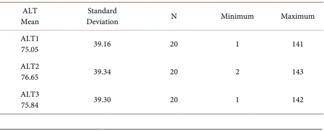
From a large tertiary hospital-based registry, the available data were grouped into female group with 20 subjects and another male group of 30 subjects. In both groups, each subject’s ALT was evaluated three times according to the rules set in [1]. The data are summarized in Table 2, for females and in Table 3 for males.

Bootstrap results

We used R to bootstrap the data. We set the number of bootstrap samples at 1000 for both data sets.

Bootstrap Statistics for females’ data: original bias std. error

0.001 0.00117 0.0004

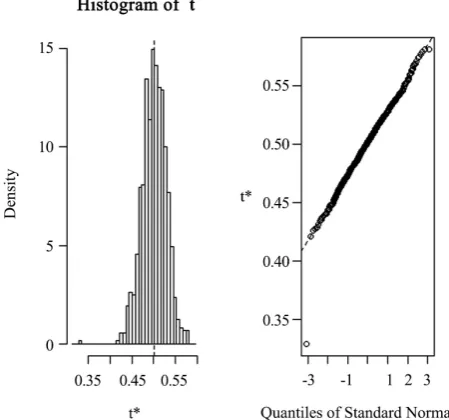
As can be seen from Figure 1, both the histogram and the Q-Q plot show that the large sample distribution of the estimator is skewed to the right. Therefore, one should be careful when constructing Wal’s confidence limits of the popula-tion RIP

Bootstrap Statistics for males’ data: original bias std. error

0.002 - 0.0001 0.0006

In contrast to females’ data, the histogram of the sample statistics as shown in

[image:9.595.210.539.606.739.2]

Figure 2 is skewed to the left, but the Q-Q plot exhibit closer to normality. This may be due to the fact that the males’ data is larger than the females’ data.

Table 2. Descriptive statistics of the female ALT data.

ALT

Mean Deviation Standard N Minimum Maximum ALT1

75.05 39.16 20 1 141

ALT2

76.65 39.34 20 2 143

ALT3

[image:10.595.219.538.89.431.2]

DOI: 10.4236/ojs.2019.94035 539 Open Journal of Statistics

Table 3. Descriptive statistics of the male ALT data.

ALT

Mean Standard Deviation N Minimum Maximum

ALT1

106.97 81.91 30 6 317

ALT2

108.87 81.96 30 8 319

ALT3

[image:10.595.259.484.481.691.2]

108.00 82.06 30 7 318

Figure 1. Histogram and the Q-Q plots of the 1000 bootstrap

samples of the estimated RIP (females ALT data).

Figure 2. Males’ data histogram and the Q-Q plots of the 1000

DOI: 10.4236/ojs.2019.94035 540 Open Journal of Statistics

7. Comments and Summary

As can be seen from the histograms and the Q-Q plots, the distribution of the es-timated RIP = t1* is far from being normally distributed. But we expect that the distributional properties may be closer to normality when the number of subjects is much larger than the number of have here. When one attempts to establish the population-based reference range of health populations, the number of subjects is typically in the hundreds, and the issue of normality may be irrelevant.

Further investigations for the case of categorical measurements and when the number of replications per subject is not fixed, are needed.

Conflicts of Interest

The authors declare no conflicts of interest regarding the publication of this pa-per.

References

[1] Bland, M. and Altman, D. (2010) Statistical-Methods for Assessing Agreement be-tween 2 Methods of Clinical Measurement. InternationalJournalof Nursing Stu-dies, 47, 931-936. https://doi.org/10.1016/j.ijnurstu.2009.10.001

[2] Shoukri, M. (2010) Measures of Interobserver Agreement and Reliability. 2nd Edi-tion, CRC Press, Taylor and Frances, Boca Raton.

[3] Shoukri, M.M. (2015) Measures of Agreement. Invited Contribution to Wiley Sta-tistical References. Stat05301.

https://doi.org/10.1002/9781118445112.stat05301.pub2

[4] Harris, E.K. and DeMets, D. (1972) Estimation of Normal Ranges and Cumulative Proportions by Transforming Observed Distributions to Gaussian Form. Clinical Chemistry, 18, 605-612.

[5] Stuart, A. and Ord, J.K. (1987) Kendall’s Advanced Theory of Statistics, Volume 1. 5th Edition, Charles Griffin, London.

[6] Shoukri, M.M., Tracy, D.S. and Mian, I.U.H. (1990) The Effect of Kurtosis in Esti-mation of the Parameters of the One-Way Random Effects Model from Familial Data. ComputationalStatisticsandDataAnalysis, 10, 339-345.

https://doi.org/10.1016/0167-9473(90)90016-B

[7] Kaplan, M.M. (2002) Alanine Aminotransferase Levels: What’s Normal? Annals of Internal Medicine, 137, 49.

https://doi.org/10.7326/0003-4819-137-1-200207020-00012

[8] Lazo, M. and Clark, J.M. (2008) The Epidemiology of Nonalcoholic Fatty Liver Disease: A Global Perspective. Seminars in Liver Disease, 28, 339-350.

https://doi.org/10.1055/s-0028-1091978

[9] Prati, D., Taioli, E., Zanella, A., Della Torre, E., Butelli, S., Del Vecchio, E., Conte, D., et al. (2002) Updated Definitions of Healthy Ranges for Serum Alanine Amino-transferase Levels. Annals of Internal Medicine, 137, 1-10.

https://doi.org/10.7326/0003-4819-137-1-200207020-00006