Abstract—Thermophoretic force and Brownian diffusion
effects were investigated on the depositions of fine particles in a turbulent boundary layer by using Eulerian-Eulerian approach. Turbulence closure was achieved by Prandtl's mixing length model. The set of equations was solved numerically by using finite difference method. Introduced particle diffusion term played a significant role in numerical convergence.Changing the temperature between plate surface and free stream indicated great influence on particle deposition. The larger particle delayed the deposition peak distance away from the plate front edge. High temperature gradient had considerable effect on flow characteristics such as skin friction factor, displacement thickness coefficient and surface density distribution.The proposed two-fluid approach for evaluating the effect of different forces on small particle deposition from a turbulent flow over a flat plate produced similar finding compared to Lagrangian method and computationally less expensive.
Index Terms—brownian, coupled gas-solid flow, diffusion
I. INTRODUCTION
HIS study involves droplet and particle deposition on a flat plate. Prediction for deposition of particle is needed in many natural and industrial processes such as microchip manufacturing, chemical coating of metals, gas filtration, and heat exchangers. In most practical applications transport occurs in the presence of turbulent flow and may be influenced by uncontrolled factors of temperature and humidity. In a flow at presence of solid surface, a boundary layer will develop and the energy and momentum transfer gives rise to temperature and velocity gradient. This convection by the bulk flow plays a significant role for particle deposition. Therefore, such flows should be model in the near wall region as accurately as possible. Generally two basic approaches are used to predict gas-solid behavior. Lagrangian method treats trajectories of individual particles and Eulerian method, the dispersed phase is regarded as a continuum and balances of mass, momentum and energy are written in differential form for both phase. A comprehensive review of both modeling approaches was reported by Crow et al. [1] when turbulence is important, the two-fluid model is computationally more efficient and
Manuscript received Feb. 22, 2012; revised March 29, 2012.
H. Basirat Tabrizi is with Mechanical Engineering Department at Amirkabir University of Technology, Hafez St. P.O. Box
15875-4413,Tehran, 159163411, Iran (corresponding author phone:
+982164543455; fax: +982166419736; e-mail: hbasirat@ aut.ac.ir).
this method is adopted for the present study. The particles on entering close to wall, deposition will occur mostly due to inertial and sedimentary mechanism. The boundary layer plays a significant role on the deposition of particles. It slows particles due to the lift forces and in problems involving heat transfer in a layer due to thermophoresis force which happens in a non-isothermal gas, in the opposite direction of the temperature gradient. Thus particles tend to move toward cold areas and be repulsed from hot areas. This phenomenon, known as thermophoresis, is of considerable importance in particle deposition problems where it can play either beneficial or adverse roles.
The case of laminar and turbulent boundary motion of gas-solid on a flat plate was discussed by Soo [2]. Kallio et al. [3] presented a Lagrangian random-walk approach to modeling particle deposition in turbulent duct flows. Particle concentration profiles reveal that smaller particles tend to accumulate in the near-wall region due to the sudden damping of fluid turbulence. Eulerian model had been employed by Taniere et al. [4] to analyze the particle motion and mass flux distributions in the mixed regime in a turbulent boundary layer two-phase flow where saltation and turbulence effects were important. Recently, particle behavior in the turbulent boundary layer of a dilute gas-particle flow was studied experimentally and numerically using CFD software by Wang et al. [5]. Their results indicated a non-uniform distribution of particle concentration with the peak value inside the turbulent boundary layer on the flat plate. They related this phenomenon to the slip-shear lift force and particle-wall collision. They used Lagrangian numerical method and did not consider the non isothermal gas effect. The slip- shear lift force effect for larger particles was shown considerable (dp = 200 μm).
Goren [6] gave a detailed theoretical analysis of thermophoretic deposition of aerosol particles in the laminar boundary layer on a flat plate. The particle concentration boundary layer due to thermophoresis had been studied for a wide range of parameters by Jayaraj [7]. Greenfield et al. [8] simulated the particle deposition in a turbulent boundary layer in the presence of thermophoresis with a test case involving heated pipe using Lagrangian approach. Kroger et al. [9] studied the deposition of log-normally distributed particles in isothermal and heated turbulent boundary layer via Lagrangian random walk simulations. The velocity and temperature fields and thermophoretic force are considered to be Gaussian random fields. Their results showed that introduction of temperature gradient lead to a strong increase in particle deposition. The deposition rate of small particles for two-dimensional turbulent gas flows onto solid
Thermophoresis of Particles over Flat Plate
Turbulent Flow based on Two-fluid Modeling
Hassan Basirat Tabrizi Member, IAENG and Golriz Kermani
weighted averaging of particle equation motion was used which generate fewer turbulence correlations. He et al. [11] developed a numerical simulation procedure for studying deposition of aerosol particles in duct flows including the effect of thermal force under laminar and turbulent conditions. A semi empirical model had been presented which covers the thermophoretic effects for the entire range of Knudsen number. Thermally enhanced deposition velocities of particles in a turbulent duct flow of a hot gas had also been evaluated.
It can be noticed most researches adopted Lagrangian approach whereby the particle equations are integrated along particle path lines. However Shahriari et al. [12] studied two-fluid modeling of turbulent boundary layer of disperse medium on a flat plate by using the particulate phase diffusivity term with the Prandtl’s mixing length theory. Further, two differential equation turbulent model was used by Gharraei et al. [13]. Small effect due to higher closure turbulence model and easy convergence due to the diffusion term for deposition of small particles was seen. Further Shahriari et al. [14] studied the effect of different temperature gradients on particle deposition across the boundary layer where Brownian effects neglected due to large size particle. In this study similar approach is applied to predict the particle behavior in gas-solid turbulent boundary layer flow on a flat plate by taking into account Brownian diffusion and thermophoresis forces. Prandtl's mixing length model is used for fluid turbulence.
II. FORMULATION AND SOLUTION
A. Governing Equations
Two-dimensional turbulent boundary layer flow of fine spherical particles-fluid suspension past a horizontal flat plate is studied via coupled two-fluid model. The fluid gas is considered to be steady, incompressible, with constant properties. The volume fraction of particulate material is assumed to be small. The Prandtl's mixing length model is used for turbulence closure model of the flowing gas. The effects of aerodynamic lift, rotation of particles on deposition are assumed to be small compare to the effect of the Brownian and thermophoretic force. The viscous, pressure terms and particle-particle collisions in the particulate phase momentum equation can be neglected. Also, the particle diffusion term is considered in this modeling. Eulerian- Eulerian approach described by Soo [2] had been modified, leading to boundary layer approximations which are applied to fluid and particle phase. List of symbols are shown in Table I. The governing equations of gas phase are:
0 y v x
uf f (1)
f p
f p f t f f f f u u F y u y y u v x u u (2) y T y y T v x T u f t t f f f f ) Pr
(
(3) Solid phase flow field are governed by:
2 2 ) ( y D D y v x u p p B p p p p
(4)
x B c p f p p p p p p p p F C u u F y u y D y u v x u u , ) ( (5)
y B Th c p f p p p p p p p p p p F F C v v F y v y y u x D y v v x v u , ) ( 2 ) ( (6) TABLEI LIST OF SYMBOLSSymbol Quantity unit
Cc Cf dp Dp
Cunningham factor friction coefficient particle diameter Particle diffusivity μm m2 /s
DB Brownian diffusivity m2
/s F
FB
Inverse relaxation Brownian force
s-1 N
Fth thermophoresis N
k Kn thermal conductivity Knudsen number w/mK
L lenth m
lm Pr Re
Prandtel mixing length Prandetl number Reynold number T U ur u,v Greek symbol p
w
temperature free stream friction velocity v velocitythermal diffusivity of particle’s material
loading ratio density
thickness
wall shear stress
K m/s m/s m/s
m2/s
N/m2
Subscript dynamic viscosity kinematic viscosity kg/ms m2/sf mp p t fluid particle mass particle turbulent
The thermophoretic force per unit particle mass can be written as (Talbot et al. [15]):
y T T d F f f mp p T f f Th
18 2 1
Where
T is a coefficient which depends on the ratio of the gas and particle thermal conductivities and Knudsen number as [15]:) 2 2 1 )( 3 1 ( ) ( 2 Kn C k k Kn C Kn C k k C t p g m t p g s T
(8)Here ,C 1.17, C 2.18 d
2
Kn s t
p
andCm1.14. The Brownian force per unit particle mass is given by Soo [2]: y D F F x D F F p p B y B p p B x B
,, ; (9)
WhereD , is the Brownian diffusion coefficient and B equal toKBT 3
dpand Cunningham correction factor,c
C , follows (see Schlichting [16]) :
1.257 0.4exp( 1.1 )
1 Kn Kn
Cc (10)
Following dimensionless quantities are introduced for numerical simulation convenience in the modeling:
U μ d L L d D T T T T T U v V U u U L y Y L x X p mp p p i i w w f f L i i i i L 18 , , Re , Re , 2 (11)
In terms of the above dimensionless quantities governing equations are expressed as:
0 Y V X
Uf f (12)
f p
p f t f f f f U U F Y U Y Y U V X U U 1 (13) Y T Y Y T V X T
U t f
t f f f f ) Pr 1 Pr 1 (
(14)
2 2 ) ( Y D D Y V XUp p p B p p
p
(15)
x B c p f f p p p p p p p p F C U U F Y U Y D Y U V X U U , ) ( (16)
y B Th c p f f p p p p p p p p p p F F C V V F Y V Y Y U X D Y V V X V U , ) ( 2 ) ( (17) Where: L mp t t t L D F L U Re 18 , Pr , Re 2
(18) Y T T T T T T T F F f w w f w T f Th ) (
(19)Y D F F X D F F p p B f y B p p B L f x B
1 , 1 Re , , (20)Turbulent or eddy viscosity,
t, is calculated by employing Prandtl’s mixing length model (see Boothroyd [17]):
Y U lLU L m f
t
Re 2
(21) 26 ) Re ( exp 1 Re 41 .
0 w f L
L m
L Y Y
l (22)
Where
wthe shear stress at the wall and the skin friction coefficient is follows:2
2
1
U
C
f w f
(23)And the dimensionless displacements thicknesses are calculated as:
0 *1 U f dY
f
(24)
0 *1 pU p dY
p
(25)
Define the thermal displacement thickness as follow;
0 *1
dy
T
T
T
T
U
u
w f w f e
(26)And in non-dimensional form is:
0 *1
T
d
Y
U
f fe
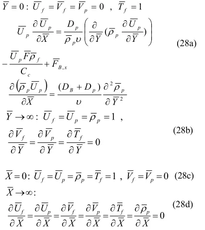
2 2 ,
) (
) (
1 , 0 :
0
Y D D
X U
F C
F U
Y U
Y D
X U U
T V
V U Y
p p B p p
x B c
f p
p p p
p p p
f p
f f
(28a)
0 , 1 :
Y T Y V Y V
U U Y
f p f
p p
f
(28b)
0 ,
1 :
0
Uf Up p Tf Vf Vp
X (28c)
0 :
X X T
X V
X V
X U
X U X
p f p f p
f
(28d)
Term,D shows particle flux due to particle diffusion and p can be estimated from the turbulent Schmidt number Sct= νt/Dt which might take values close to unity or else. The effect of particle diffusion term was discussed without thermophoresis and Brownian force elsewhere (see Shahriari et al. [14]).
B. Numerical Procedure
The hydrodynamic and thermal boundary layer equations (12 to 17) and their boundary conditions are solved numerically using finite difference scheme. A two-dimensional logarithmic mesh form is superimposed on the flow field. Different mesh sizes are compared to obtain grid-independent results for inlet velocity of 20 m/s and 2.5 µm particle sizes. It is shown in Fig. 1 maximum error due to different computational mesh sizes reveals in the near-wall region. A 100x140 mesh is selected as the optimum mesh regarding to the computational time. The minimum value of
y
has set to be 0.03. Coarse mesh sizes lead to unphysical results and convergence problems.
Gas and particle continuity equations and boundary condition for particle density along the plate are solved implicitly while other governing equations and boundary conditions are implied explicitly. Computation proceeds up to the steady state which is considered to reach for a relative change of field variables less than10-6.
III. RESULTSANDDISCUSSION
As stated earlier, there is no coupled two-fluid approach for this kind of study even without the diffusion part, so the model predictions without the thermophoresis effect have been compared to only available experimental and theoretical results of Taniere et al. [4]. Here, the physical property of those reported is used for the model simulation. Inlet velocity of 10.6 m/s, particle size and density of 60 micron and 2500 Kg/m3, loading ratio of 0.1 at location of 1.89m.
[image:4.612.85.291.48.279.2][image:4.612.322.474.48.491.2]
Fig.1. Mesh Comparison
Figure 2 indicates this comparison. The particle diffusion term used in the present model is taken to be equal to the thermal diffusivity of particle material (for glass, Dp =
0.05). The velocities,
u
u
u
are expressed in wall distance unit,
y
yu
Fig.2. Model comparison of Gas and particle mean velocity profiles with Taniere et al. [4]
Numerical simulation is carried withDp = 0.05, loading ratio of 1.0, particle size and density of 2.5 µm and 2500 Kg/m3 respectively unless is stated something else. Also, in this study, we concentrate on the skin friction coefficient, displacement thickness and thermal displacement thickness effect which are important for design consideration.
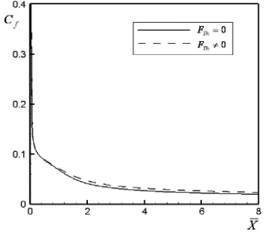
Figure 3 compares the effect of thermophoresis force on the flat plate for temperature difference of 300K. It indicates lower skin friction coefficient due to thermophoresis force. Effect of different temperature on the skin friction is shown in Fig. 4. It can be noticed, the negative temperature difference gives higher skin friction coefficient compare to the positive temperature difference. This means while the wall temperature is higher, the friction coefficient becomes higher due to increase of particle density on the surface. Fig. 5 shows for smaller size particle due to higher deposition, the skin friction factor is higher than larger size particle for temperature difference of 50 K.
The displacement thickness for gas and particle with temperature difference of 300 K is shown in Fig. 6. It appears that the thermophoresis force lower the displacement thickness due to higher concentration of particles.
Fig.3. Effect of thermophoresis on skin friction coefficient
[image:5.612.69.283.48.207.2]Fig.4. Temperature difference effect on the skin friction coefficient
[image:5.612.322.536.262.447.2]Fig.5. Particle size effect on the skin friction coefficient
Fig.6. Displacement thickness effect for gas and particle phase
[image:5.612.319.534.476.658.2] [image:5.612.92.285.513.683.2]The effect of surface particle density distribution with and without thermophoresis force is shown in Fig. 8 for temperature difference of 300 K. Higher deposition is seen with thermophoresis force. Also, it indicates higher value for the smaller size particle and closer to the entrance region.
Fig.7. Thermal displacement thickness
Fig.8. Surface particle density distribution
IV. CONCLUSION
The effect of thermophoresis and Brownian force was carried out for turbulent flow on a horizontal flat plate by using the two-way coupling Eulerian-Eulerian approach. Prandtl mixing length theory was used as closure model of turbulence. In addition, for the particle deposition at the wall the particle diffusion term was introduced. The governing equations were solved by a finite difference method. As a result of the thermophoretic force, particle deposition increased which was predicted by using other kind of approaches such as Eulerian-Lagrangian [8]. Presenting the dispersed phase within the concept of Eulerian approach and adding the particle diffusion term for the dispersed phase, the problem of convergence was solved much easier.
Changing the temperature difference between plate surface and free stream had great influence on particle deposition on the flat plate. The larger particle delayed the deposition peak further distance away from the plate front edge. The skin friction coefficient increased and the displacement thickness decreased. This can be considered in design criteria. Also, the current approach on small particle
deposition from a turbulent flow over a flat plate uses less computing time and memories.
REFERENCES
[1] C. T. Crowe and J. N. Trout, “Numerical models for two-phase turbulent flows,” Ann. Rev. Fluid mechanics, vol. 28, pp. 11-43, 1996. [2] S. L. Soo, Particulates and Continuum, Multiphase Fluid Dynamics
HPC, 1989.
[3] G. A. Kallio and M. W. Reeks, “A numerical simulation of particle deposition in turbulent boundary layers, ” Int. J. Multiphase flow, vol. 15, no. 3, pp. 433-446, 1989.
[4] A. Taniere, B. Oesterle and J. M. Foucaut, “Modeling of saltation and turbulence effects in a horizontal gas-solid boundary layer,” Particulate Science and Technology, vol. 14, pp. 337-350, 1997. [5] J. Wang and E. K. Levy, “Particle behavior in the turbulent boundary
layer of a dilute gas-particle flow past a flat plate,” Exp. Thermal Fluid Science, vol. 30, pp. 473-483, 2006.
[6] S. L. Goren, “Thermophoresis of aerosol particles in the laminar boundary layer on a flat surface,” J. Colloid Interface Sci., vol. 61, pp. 77-85, 1977.
[7] S. Jayaraj, “Thermophoresis in laminar flow over cold inclined plates with variable properties,” Heat and Mass Transfer, vol. 30, pp. 167-173, 1995.
[8] C. Greenfield and G. Quarini, “A Lagrangian simulation of particle deposition in a turbulent boundary layer in the presence of thermpphoresis,” Applied Mathematical Modeling, vol. 22, pp. 759-771, 1998.
[9] C. Kroger and Y. Drossinos, “A random-walk simulation of thermophoretic particle deposition in a turbulent boundary layer,” Int. J. Multiphase Flow, vol. 26, pp. 1325-1350, 2000.
[10] S. A. Slater, A. D. Leeming and J. B. Young, “Particle deposition from two-dimensional turbulent gas flows,” Int. Multiphase flow, vol. 29, pp. 721-750, 2003.
[11] C. He and G. Ahmadi, “Particle deposition with thermophoresis in laminar and turbulent duct flows,” Aerosol Sci. and Tech., vol. 29, pp. 525-546, 1998.
[12] Sh. Shahriari and H. Basirat Tabrizi, “Modeling of Turbulent Boundary Layer of a Disperse medium on a Flat Plate, ” Proceedings of the IASTED2003, Int. Conference, Applied Simulation and Modeling, ISBN:0-88986-384-9, ACTA Press, pp.7-12.
[13] R. Gharraei, H. Basirat Tabrizi, and E. Esmaeilzadeh, “Prediction of Turbulent Boundary Layer Flow of a Particulate Suspension Using κ-τ Model ” CSME2004 Forum, the Canadian Society for Mechanical Engineering Proceedings, pp.29-35.
[14] Sh. Shahriari and H. Basirat Tabrizi, “Two-fluid Model Simulation of Thermophorestic Deposition for Fine Particles in a Turbulent Boundary Layer,” ASME-JSME2007 Thermal Engineering Summer Heat Transfer Conf., HT2007-32117, vol. 2, pp. 849-854.
[15] L. Talbot, R. K. Cheng, R. W. Schefer and D. R. Willis, “Therophoresis of particles in a heated boundary layer, ” J. Fluid Mech., vol. 101, pp. 737-758, 1980.
[16] H. Schlichting, Boundary Layer Theory, New York: McGraw-Hill, 1979.