Generalizing Case Frames Using a Thesaurus and the MDL Principle

(1)

Generalizing Case Frames Using a

Thesaurus and the MDL Principle

H a n g Li* NEC Corporation

N a o k i A b e * NEC Corporation

A new method for automatically acquiring case frame patterns from large corpora is proposed. In particular, the problem of generalizing values of a case frame slot for a verb is viewed as that of estimating a conditional probability distribution over a partition of words, and a new generalization method based on the Minimum Description Length (MDL) principle is proposed. In order to assist with efficiency, the proposed method makes use of an existing thesaurus and restricts its attention to those partitions that are present as "cuts" in the thesaurus tree, thus reducing the generalization problem to that of estimating a "tree cut model" of the thesaurus tree. An efficient algorithm is given, which provably obtains the optimal tree cut model for the given frequency data of a case slot, in the sense of MDL. Case frame patterns obtained by the method were used to resolve PP-attachment ambiguity. Experimental results indicate that the proposed method improves upon or is at least comparable with existing methods.

1. Introduction

We address the problem of automatically acquiring case frame patterns (selectional patterns, subcategorization patterns) from large corpora. A satisfactory solution to this problem would have a great impact on various tasks in natural language processing, including the structural disambiguation problem in parsing. The acquired knowledge would also be helpful for building a lexicon, as it would provide lexicographers with word usage descriptions.

In our view, the problem of acquiring case frame patterns involves the following two issues: (a) acquiring patterns of individual case frame slots; and (b) learning dependencies that may exist between different slots. In this paper, we confine ourselves to the former issue, and refer the interested reader to Li and Abe (1996), which deals with the latter issue.

The case frame (case slot) pattern acquisition process consists of two phases: extrac- tion of case frame instances from corpus data, and g e n e r a l i z a t i o n of those instances to case frame patterns. The generalization step is needed in order to represent the input case frame instances more compactly as well as to judge the (degree of) acceptability of unseen case frame instances. For the extraction problem, there have been various methods proposed to date, which are quite adequate (Hindle and Rooth 1991; Grish- man and Sterling 1992; Manning 1992; Utsuro, Matsumoto, and Nagao 1992; Brent 1993; Smadja 1993; Grefenstette 1994; Briscoe and Carroll 1997). The generalization problem, in contrast, is a more challenging one and has not been solved completely. A number of methods for generalizing values of a case frame slot for a verb have been

(2)

Computational Linguistics Volume 24, Number 2

proposed. Some of these methods make use of prior knowledge in the form of an existing thesaurus (Resnik 1993a, 1993b; Framis 1994; Almuallim et al. 1994; Tanaka 1996; Utsuro and Matsumoto 1997), while others do not rely on any prior knowledge (Pereira, Tishby, and Lee 1993; Grishman and Sterling 1994; Tanaka 1994). In this paper, we propose a new generalization method, belonging to the first of these two categories, which is both theoretically well-motivated and computationally efficient.

Specifically, we formalize the problem of generalizing values of a case frame slot for a given verb as that of estimating a conditional probability distribution over a partition of words, and propose a new generalization method based on the Minimum Description Length principle (MDL): a principle of data compression and statistical estimation from information theory. 1 In order to assist with efficiency, our method makes use of an existing thesaurus and restricts its attention on those partitions that are present as "cuts" in the thesaurus tree, thus reducing the generalization problem to that of estimating a "tree cut model" of the thesaurus tree. We then give an efficient algorithm that provably obtains the optimal tree cut model for the given frequency data of a case slot, in the sense of MDL. In order to test the effectiveness of our method, we conducted PP-attachment disambiguation experiments using the case frame patterns obtained by our method. Our experimental results indicate that the proposed method improves upon or is at least comparable to existing methods.

The remainder of this paper is organized as follows: In Section 2, we formalize the problem of generalizing values of a case frame slot as that of estimating a conditional distribution. In Section 3, we describe our MDL-based generalization method. In Sec- tion 4, we present our experimental results. We then give some concluding remarks in Section 5.

2. The Problem

2.1 The Data Sparseness Problem

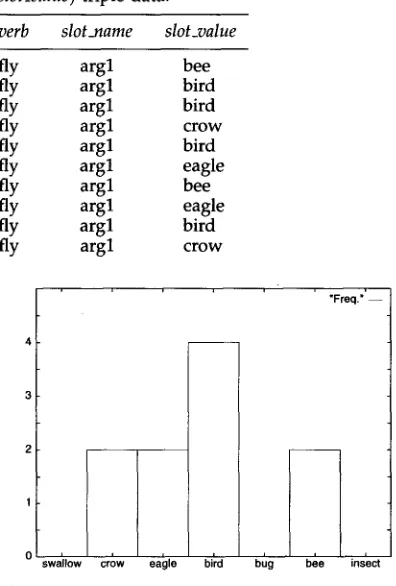
Suppose that the data available to us are of the type shown in Table 1, which are slot values for a given verb

(verb,slot_name,slot_value

triples) automatically extracted from a corpus using existing techniques. By counting the frequency of occurrence of each noun at a given slot of a verb, the frequency data shown in Figure 1 can be obtained. We will refer to this type of data as co-occurrence data. The problem of generalizing values of a case frame slot for a verb (or, in general, a head) can be viewed as the problem of learning the underlying conditional probability distribution that gives rise to such co-occurrence data. Such a conditional distribution can be represented by a probability model that specifies the conditional probability

P(n I v, r)

for each n in the set of nouns .M = {nl, n2 . . . nN}, V in the set of verbs V = {vl, v2 . . .

Vv},

and r in the set of slot names T~ =

{rl,

r2 . . . rR}, satisfying:

P(n

Iv, r) = 1. (1)

nGM

This type of probability model is often referred to as a word-based model. Since the number of probability parameters in word-based models is large (O(N. V. R)), accurate

(3)

Li and Abe Generalizing Case Frames

Table 1

Example

(verb, slot_name,

slot_value)

triple data.

verb

slot_name slot_value

fly argl bee

fly argl bird

fly argl crow

fly argl bird

fly argl eagle

fly argl bee

fly argl eagle

fly argl bird

fly argl crow

"Freq." - -

swallow crow eagle bird bug bee insect Figure 1

Frequency data for the subject slot of verb

fly.

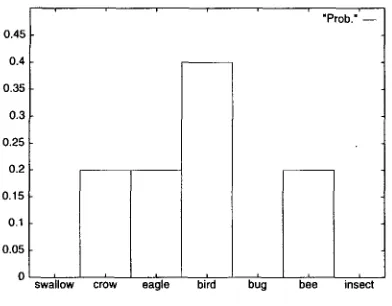
estimation of a word-based model is difficult with the data size that is available in practice--a problem usually referred to as the data sparseness problem. For example, suppose that we employ the maximum-likelihood estimation (or MLE for short) to estimate the probability parameters of a conditional probability distribution, as described above, given the co-occurrence data in Figure 1. In this case, MLE amounts to estimating the parameters by simply normalizing the frequencies so that they sum to one, giving, for example, the estimated probabilities of 0, 0.2, and 0.4 for

swallow,

eagle,

and

bird,

respectively (see Figure 2). Since in general the number of parameters exceeds the size of data that is typically available, MLE will result in estimating most of the probability parameters to be zero.

[image:3.468.36.234.93.386.2]

(4)

"Prob." - - 0.45

0.4

0.35

0.3

0.25

0.2

0.15

0.1

0.05

0

swallow crow eagle bird bug bee insect

Figure 2

Word-based distribution estimated using MLE.

models, which assign (conditional) probability values to (existing) classes of words, rather than individual words.

2.2 Class-based Models

An example of the class-based approach is Resnik's m e t h o d of generalizing values of a case frame slot using a thesaurus a n d the so-called selectional association measure (Resnik 1993a, 1993b). The selectional association, d e n o t e d

A(C I v,

r), is defined as follows:

P ( C I v , r)

(2)

A(C I v, F) = P(C I v, F)

x log

P(C)

where C is a class of n o u n s present in a given thesaurus, v is a verb a n d r is a slot name, as described earlier. In generalizing a given n o u n n to a n o u n class, this m e t h o d selects the n o u n class C having the

maximum

A(C I v, r), a m o n g all super classes of n in a given thesaurus. This m e t h o d is based on an interesting intuition, b u t its interpretation as a m e t h o d of estimation is not clear. We propose a class-based generalization m e t h o d whose performance as a m e t h o d of estimation is guaranteed to be near optimal.

We define the class-based m o d e l as a model that consists of a partition of the set .N" of nouns, a n d a parameter associated w i t h each m e m b e r of the partition. Here, a partition F of .M is a n y collection of m u t u a l l y disjoint subsets of iV" that exhaustively cover N . The parameters specify the conditional probability P(C I v, r) for each class (subset) C in that partition, such that

P ( C I v , r)

= 1. (3)

CEF

Within a given class C, it is a s s u m e d that each n o u n is generated w i t h equal probability, n a m e l y

1

Vn E C: P(n l v, r) = ~

x P(C I v, F).

(4)

[image:4.468.54.250.50.203.2]

(5)

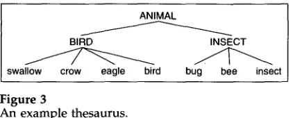
ANIMAL

BIRD INSECT

swallow crow eagle bird bug bee insect

Figure 3

An example thesaurus.

case-pattern acquisition process. It is also possible to e x t e n d o u r m o d e l so that each w o r d probabilistically belongs to several different classes, w h i c h w o u l d allow us to resolve b o t h structural a n d w o r d - s e n s e ambiguities at the time of disambiguation. 2 E m p l o y i n g probabilistic m e m b e r s h i p , however, w o u l d m a k e the estimation process significantly m o r e c o m p u t a t i o n a l l y d e m a n d i n g . We therefore leave this issue as a future topic, a n d e m p l o y a simple heuristic of equally distributing each w o r d occurrence in the data to all of its potential w o r d senses in o u r experiments. Since o u r learning m e t h o d based on MDL is robust against noise, this s h o u l d n o t significantly d e g r a d e performance.

2.3 The Tree Cut M o d e l

Since the n u m b e r of partitions for a given set of n o u n s is e x t r e m e l y large, the p r o b l e m of selecting the best m o d e l from a m o n g all possible class-based m o d e l s is m o s t likely intractable. In this paper, w e r e d u c e the n u m b e r of possible partitions to consider b y using a t h e s a u r u s as p r i o r k n o w l e d g e , following a basic idea of Resnik's (1992).

In particular, we restrict o u r attention to those partitions that exist within the thesaurus in the f o r m of a cut. By thesaurus, w e m e a n a tree in w h i c h each leaf n o d e stands for a n o u n , while each internal n o d e represents a n o u n class, a n d d o m i n a t i o n stands for set inclusion (see Figure 3). A cut in a tree is a n y set of n o d e s in the tree that defines a partition of the leaf nodes, v i e w i n g each n o d e as representing the set of all leaf n o d e s it dominates. For example, in the thesaurus of Figure 3, there are five cuts: [ANIMAL], [BIRD, INSECT], [BIRD, bug, bee, insect], [swallow, crow, eagle, bird, INSECT], a n d [swallow, crow, eagle, bird, bug, bee, insect]. The class of tree cut m o d e l s of a fixed thesaurus tree is then obtained b y restricting the partition P in the definition of a class-based m o d e l to be those partitions that are p r e s e n t as a cut in that thesaurus tree.

Formally, a tree cut m o d e l M can be r e p r e s e n t e d b y a pair consisting of a tree cut lP a n d a probability p a r a m e t e r vector 0 of the same length, that is:

V = (r, e) (5)

w h e r e lP a n d 0 are:

r = [C1, C2 . . . Ck+l], e = [P(C1), P(C2) . . .

P(Ck+l)]

(6)

k+l

w h e r e C1, C2 . . .

Ck+l

is a cut in the thesaurus tree a n d ~i=1

P(Ci)

= 1 is satisfied. For simplicity w e sometimes write

P(Ci),

i = 1 . . . (k + 1) for

P(Ci [ v, r).

If w e use MLE for the p a r a m e t e r estimation, w e can obtain five tree cut m o d e l s from the co-occurrence data in Figure 1; Figures 4-6 s h o w three of these. For example,

[image:5.468.36.247.50.135.2]

(6)

Computational Linguistics Volume 24, Number 2

0.45

0.4

0.35

0.3

0.25

0.2

0.15

0.1

0.05

0

- r ~ - ' - - - ~ - - ~ ,Prob r-'~--

swallow crow eagle bird bug bee insect Figure 4

A tree cut model with [swallow, crow, eagle, bird, bug, bee, insect].

0.45

0.4

0.35

0.3

0.25

0.2

0.15

0.1

0.05

0

"Prob."

swa'll . . . . ow eagle bi'rd bug bee ins'ect

Figure 5

A tree cut model with [BIRD, bug, bee, insect].

~- ([BIRD, bug, bee, insect], [0.8,0,0.2,0]) s h o w n in Figure 5 is one such tree cut

model. Recall that M defines a conditional probability distribution

PM(n I v,r)

as

follows: For any noun that is in the tree cut, such as

bee,

the probability is given as

explicitly specified by the model, i.e., PM(bee I flY, argl) = 0.2. For any class in the tree cut, the probability is distributed uniformly to all nouns dominated by it. For example,

since there are four nouns that fall under the class BIRD, and

swallow

is one of them,

the probability of

swallow

is thus given by Pt~(swallow I flY, argl) = 0.8/4 = 0.2. Note

that the probabilities assigned to the nouns under BIRD are smoothed, even if the nouns have different observed frequencies.

We have thus formalized the problem of generalizing values of a case frame slot as that of estimating a model from the class of tree cut models for some fixed thesaurus tree; namely, selecting a model that best explains the data from among the class of tree cut models.

3. Generalization Method Based On M D L

The question n o w becomes what strategy (criterion) w e should employ to select the

best

[image:6.468.55.251.49.199.2] [image:6.468.55.250.233.385.2]

(7)

0.45 0.4 0,35 0,3 0.25 0.2 O,lS 0.1 0,05

[image:7.468.40.379.47.228.2]

0 swallow crow eagle bi'rd

Figure 6

A tree cut model with [BIRD, INSECT].

"Prob." - -

Table 2

Number of parameters and KL distance from the empirical distribution for the five tree cut models.

P Number of Parameters KL Distance

[ANIMAL] [BIRD, INSECT] [BIRD, bug, bee, insect]

[swallow, crow, eagle, bird, INSECT] [swallow, crow, eagle, bird, bug, bee, insect]

0 0.89

1 0.72

3 0.4

4 0.32

6 0

1983, 1984, 1986, 1989), w h i c h has various desirable properties, as will be described later. 3

MDL is a principle of data c o m p r e s s i o n a n d statistical estimation from information theory, w h i c h states that the best probability m o d e l for given data is that w h i c h requires the least code length in bits for the e n c o d i n g of the m o d e l itself a n d the g i v e n data o b s e r v e d t h r o u g h it. 4 The f o r m e r is the model description length a n d the latter the data description length.

In o u r current problem, it tends to be the case, in general, that a m o d e l nearer the root of the thesaurus tree, such as that in Figure 6, is simpler (in terms of the n u m b e r of parameters), b u t tends to h a v e a p o o r e r fit to the data. In contrast, a m o d e l nearer the leaves of the thesaurus tree, such as that in Figure 4, is m o r e complex, b u t tends to h a v e a better fit to the data. Table 2 s h o w s the n u m b e r of free p a r a m e t e r s a n d the KL distance from the empirical distribution of the data (namely, the w o r d - b a s e d distribution estimated b y MLE) s h o w n in Figure 2 for each of the five tree cut models. 5 In the table, one can see that there is a trade-off b e t w e e n the simplicity of a m o d e l a n d the g o o d n e s s of fit to the data.

In the M D L f r a m e w o r k , the m o d e l description length is an indicator of m o d e l

3 Estimation strategies related to MDL have been independently proposed and studied by various authors (Solomonoff 1964; Wallace and Boulton 1968; Schwarz 1978; Wallace and Freeman 1992). 4 We refer the interested reader to Quinlan and Rivest (1989) for an introduction to the MDL principle. 5 The KL distance (alsO known as KL-divergence or relative entropy), which is widely used in

(8)

complexity, while the data description length indicates goodness of fit to the data. The MDL principle stipulates that the model that minimizes the sum total of the description lengths should be the best model (both for data compression and statistical estimation). In the remainder of this section, we will describe how we apply MDL to our current problem. We will then discuss the rationale behind using MDL in our present context.

3.1 C a l c u l a t i n g D e s c r i p t i o n L e n g t h

We first show how the description length for a model is calculated. We use S to denote a sample (or set of data), which is a multiset of examples, each of which is an occurrence of a noun at a given slot r of a given verb v (i.e., duplication is allowed). We let ISI denote the size of S as a multiset, and n E S indicate the inclusion of n in S as a multiset. For example, the column labeled

slot_value

in Table 1 represents a sample S for the subject slot offly, and in this case ISI = 10.

Given a sample S and a tree cut F, we employ MLE to estimate the parameters of the corresponding tree cut model ~,I = (F, 0), where 6 denotes the estimated parameters.

The total description length L(/~,I, S) of the tree cut model/vl and the sample S observed through M is computed as the sum of the model description length L(P), parameter description length L(0 I P), and data description length

L(S I F,

6):

L(M,S) = L((F,6),S) = L(r) + L(6 I r)

+L(Str,6).

(7) Note that we sometimes refer to L(F) + L(0 I F) as the model description length.

The model description length L(F) is a subjective quantity, which depends on the coding scheme employed. Here, we choose to assign the same code length to each cut and let:

L(F)

= log IG[ (8)

where ~ denotes the set of all cuts in the thesaurus tree T. 6 This corresponds to assuming that each tree cut model is equally likely a priori, in the Bayesian interpretation of MDL. (See Section 3.4.)

The parameter description length

L(O I F)

is calculated by: k

L(0 I r) = ~

x log IsI (9)

where ISI denotes the sample size and k denotes the number of free parameters in the tree cut model, i.e., k equals the number of nodes in P minus one. It is known to be best to use this number of bits to describe probability parameters in order to minimize the expected total description length (Rissanen 1984, 1986). An intuitive explanation of this is that the standard deviation of the maximum-likelihood estimator of each parameter is of the order ~ , and hence describing each parameter using more than 1 1 log ISI bits would be wasteful for the estimation accuracy possible with - l o g x / ~ - 2

the given sample size.

Finally, the data description length

L(S I

F, 0) is calculated by:

L(S

I r, 0) = - ~ log P(n) (10)

nES

(9)

[image:9.468.32.227.77.209.2]

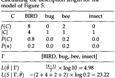
Table 3

Calculating the description length for the model of Figure 5.

C B I R D bug bee insect

f(C)

8

0

2

0

ICI 4 1 1 1

P(C) 0.8 0.0 0.2 0.0

P(n) 0.2 0.0 0.2 0.0

P [BIRD, bug, bee, insect] L(0

1 r)

(47l)

x log 10 = 4.98

L(S I P,~)

- ( 2 + 4 + 2 + 2 ) x log0.2 = 23.22

where for simplicity we write P(n) for

PM(n [ v, r).

Recall that P(n) is obtained b y MLE, namely, b y normalizing the frequencies:

1

P(n) = ~ x P(C) (11)

for each C c P a n d each n E C, where for each C c P:

= d ( C )

(12)

ISI

w h e r e f ( C ) denotes the total frequency of n o u n s in class C in the sample S, a n d F is a tree cut. We note that, in fact, the maximum-likelihood estimate is one that minimizes the data description length

L(S I F, 0).

With description length defined in the above manner, we wish to select a model with the m i n i m u m description length and o u t p u t it as the result of generalization. Since we assume here that every tree cut has an equal L(P), technically we need only calculate a n d compare L'(/[d, S) = L(~ I F) +

L(S t

F, ~) as the description length. For simplicity, we will sometimes write just L'(F) for L'(7[/I, S), where I ~ is the tree cut of M, w h e n ~,I a n d S are clear from context.

The description lengths for the data in Figure 1 using various tree cut models of the thesaurus tree in Figure 3 are s h o w n in Table 4. (Table 3 shows h o w the description length is calculated for the model of tree cut ]BIRD, bug, bee, insect].) These figures indicate that the model in Figure 6 is the best model, according to MDL. Thus, given the data in Table 1 as input, the generalization result s h o w n in Table 5 is obtained.

3.2 An Efficient Algorithm

(10)

Table 4

Description length of the five tree cut models.

r L(~ I r) L(S ] r,~) L'(P)

[ANIMAL] 0 28.07 28.07

[BIRD, INSECT] 1.66 26.39 28.05

[BIRD, bug, bee, insect] 4.98 23.22 28.20

[swallow, crow, eagle, bird, INSECT] 6.64 22.39 29.03 [swallow, crow, eagle, bird, bug, bee, insect] 9.97 19.22 29.19

Table 5

Generalization result.

verb slot~name slot_value probability

fly argl BIRD 0.8

fly argl INSECT 0.2

Here w e let t denote a thesaurus (sub)tree, root(t) the root of the tree t. Initially t is set to the entire tree.

Also input to the algorithm is a co-occurrence data.

algorithm Find-MDL(t) := cut

1. if

2. t is a leaf n o d e

3. t h e n

4. retum([t])

5. else

6. For each child tree ti of t ci :=Find-MDL(ti) 7. c:= append(ci)

8. if

9. L'([root(t)]) < L'(c)

10. t h e n

11. return([root(t)])

12. else

13. return(c)

Figure 7

The algorithm: Find-MDL.

simple and efficient algorithm b a s e d on dynamic programming, which is guaranteed to find a m o d e l with the m i n i m u m description length.

Our algorithm, which w e call Find-MDL, recursively finds the optimal M D L m o d e l for each child subtree of a given tree and a p p e n d s all the optimal models of these subtrees and returns the a p p e n d e d models, unless collapsing all the lowerqevel optimal models into a m o d e l consisting of a single n o d e (the root n o d e of the given tree) re- duces the total description length, in which case it does so. The details of the algorithm are given in Figure 7. N o t e that for simplicity w e describe Find-MDL as outputting a tree cut, rather than a complete tree cut model.

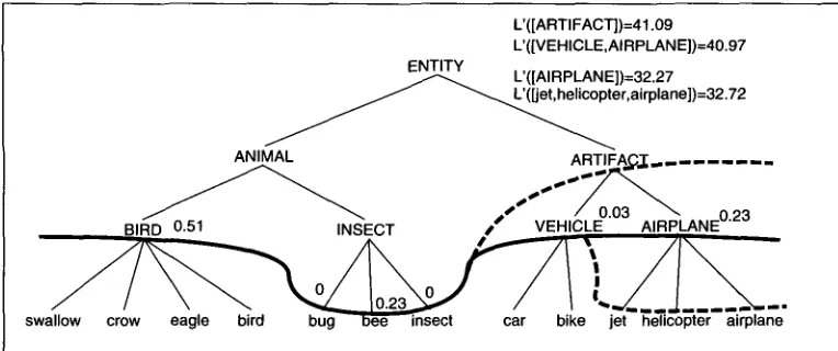
[image:10.468.51.362.73.256.2] [image:10.468.54.363.263.505.2]

(11)

L'([ARTIFACT])=41.09

L'([VEHICLE,AIRPLANE])=40.97 ENTITY

L'([AIR PLAN E])=32.27

r,airplane])=32.72

R O ~ i N S

_..

A

_7o.2-..

a ~ 5A'C"I .. . .

• 0.23

BI CT l VEHICLE AIRPLANE

swallow crow eagle bird bug ~lS~"~insect car bike jet helicopter airplane

f(swallow)=4,f(crow)=4,f(eagle)=4,f(bird)=6,f(bee)=8,f(car)=l ,f(jet)=4,f(airplane)=4

Figure 8

An example application of Find-MDL.

log ISI, where k + 1 is the number of nodes in the current cut, both when t is the 2

entire tree and when it is a proper subtree. This contrasts with the fact that the number of free parameters is k for the former, while it is k + 1 for the latter. For the purpose of finding a tree cut with the minimum description length, however, this distinction can be ignored (see Appendix A).

Figure 8 illustrates h o w the algorithm works (on the co-occurrence data shown at the bottom): In the recursive application of Find-MDL on the subtree rooted at AIRPLANE, the if-clause on line 9 evaluates to true since L'([AIRPLANE]) = 32.27, L'(~et, helicopter, airplane]) = 32.72, and hence [AIRPLANE] is returned. Then in the call to Find-MDL on the subtree rooted at ARTIFACT, the same if-clause evaluates to false since L'([VEHICLE, AIRPLANE]) = 40.97, L'([ARTIFACT]) = 41.09, and hence [VEHICLE, AIRPLANE] is returned.

Concerning the above algorithm, we show that the following proposition holds:

Proposition 1

The algorithm Find-MDL terminates in time

O(N

x ISI), where N denotes the number of leaf nodes in the input thesaurus tree T and ISI denotes the input sample size, and outputs a tree cut model of T with the minimum description length (with respect to the encoding scheme described in Section 3.1).

[image:11.468.34.416.47.207.2]

(12)

consisting of the root of the tree or the model obtained by appending the optimal submodels for its child subtrees. 7

3.3 Estimation, Generalization, and MDL

When a discrete model (a partition F of the set of nouns W" in our present context) is fixed, and the estimation problem involves only the estimation of probability parameters, the classic maximum-likelihood estimation (MLE) is known to be satisfactory. In particular, the estimation of a word-based model is one such problem, since the partition is fixed and the size of the partition equals [.M[. Furthermore, for a fixed discrete model, it is known that MLE coincides with MDL: Given data S = {xi : i = 1 . . . m } ,

MLE estimates parameter P, which maximizes the likelihood with respect to the data; that is:

m

= arg mpax H P(xi). (13)

i=1

It is easy to see that P also satisfies:

m

= arg nun ~ - log P(xi). (14)

i=1

This is nothing but the MDL estimate in this case,

since ~i~1 -log

P(xi) is the data description length.

When the estimation problem involves model selection, i.e., the choice of a tree cut in the present context, MDUs behavior significantly deviates from that of MLE. This is because MDL insists on minimizing the sum total of the data description length

and the model description length, while MLE is still equivalent to minimizing the data description length only. So, for our problem of estimating a tree cut model, MDL tends to select a model that is reasonably simple yet fits the data quite well, whereas the model selected by MLE will be a word-based model (or a tree cut model equivalent to the word-based modelS), as it will always manage to fit the data.

In statistical terms, the superiority of MDL as an estimation method is related to the fact we noted earlier that even though MLE can provide the best fit to the given data, the estimation accuracy of the parameters is poor, when applied on a sample of modest size, as there are too m a n y parameters to estimate. MLE is likely to estimate most parameters to be zero, and thus suffers from the data sparseness problem. Note in Table 4, that MDL avoids this problem by taking into account the model complexity as well as the fit to the data.

MDL stipulates that the model with the m i n i m u m description length should be selected both for data compression and estimation. This intimate connection between estimation and data compression can also be thought of as that between estimation and generalization, since in order to compress information, generalization is necessary. In our current problem, this corresponds to the generalization of individual nouns present in case frame instances in the data as classes of nouns present in a given thesaurus. For example, given the thesaurus in Figure 3 and frequency data in Figure 1, we would

7 The process of finding the MDL m o d e l tends to be computationally d e m a n d i n g a n d is often

intractable. W h e n the m o d e l class u n d e r consideration is restricted to tree structures, however, d y n a m i c p r o g r a m m i n g is often applicable a n d the MDL m o d e l can be efficiently found. For example, Rissanen (1995) has d e v i s e d an algorithm for learning decision trees.

(13)

like our system to judge that the class BIRD and the noun

bee

can be the subject slot of the verb

fly.

The problem of deciding whether to stop generalizing at BIRD and

bee,

or generalizing further to ANIMAL has been addressed by a number of authors (Webster and Marcus 1989; Velardi, Pazienza, and Fasolo 1991; Nomiyama 1992). Minimization of the total description length provides a disciplined criterion to do this.

A remarkable fact about MDL is that theoretical findings have indeed verified that MDL, as an estimation strategy, is near optimal in terms of the rate of convergence of its estimated models to the true model as data size increases. When the true model is included in the class of models considered, the models selected by MDL converge to the true model at the rate of O/~C:~9~_i~!~ where k* is the number of parameters in _2.1Sl _J' the true model, and [S] the data

size,

which is near optimal (Barron and Cover 1991; Yamanishi 1992).

Thus, in the current problem, MDL provides (a) a w a y of smoothing probability parameters to solve the data sparseness problem, and at the same time, (b) a w a y of generalizing nouns in the data to noun classes of an appropriate level, both as a corollary to the near optimal estimation of the distribution of the given data.

3.4 The Bayesian Interpretation of MDL and the Choice of Encoding Scheme

There is a Bayesian interpretation of MDL: MDL is essentially equivalent to the "posterior mode" in the Bayesian terminology (Rissanen 1989). Given data S and a number of models, the Bayesian estimator (posterior mode) selects a model M that maximizes the posterior probability:

= a r g n ~ x ( P ( M ) .

P(S

I M ) ) (15) where

P(M)

denotes the prior probability of the model M and

P(S [ M)

the probability of observing the data S given M. Equivalently, M satisfies

~'I = argn~m(- logP(M) - logP(S I M)). (16) This is equivalent to the MDL estimate, if we take - log

P(M)

to be the model description length. Interpreting - log

P(M)

as the model description length translates, in the Bayesian estimation, to assigning larger prior probabilities on simpler models, since it is equivalent to assuming that

P(M)

= (½)t(a), where

I(M)

is the description length of M. (Note that if we assign uniform prior probability

P(M)

to all models M, then (15) becomes equivalent to (13), giving the maximum-likelihood estimate.)

Recall, that in our definition of parameter description length, we assign a shorter parameter description length to a model with a smaller number of parameters k, which admits the above interpretation. As for the model description length (for tree cuts) we assigned an equal code length to each tree cut, which translates to placing no bias on any cut. We could have employed a different coding scheme assigning shorter code lengths to cuts nearer the root. We chose not to do so partly because, for sufficiently large sample sizes, the parameter description length starts dominating the model description length anyway.

(14)

Find-MDL m a y not exist. We believe that o u r choice of m o d e l description length is d e r i v e d from a natural e n c o d i n g scheme with reasonable interpretation as Bayesian prior, a n d at the same time allows an efficient algorithm for finding a m o d e l w i t h the m i n i m u m description length.

3.5 The Uniform Distribution A s s u m p t i o n and the Level of Generalization

The u n i f o r m distribution a s s u m p t i o n m a d e in (4), n a m e l y that all n o u n s b e l o n g i n g to a class contained in the tree cut m o d e l are assigned the same probability, seems to be rather stringent. If one w e r e to insist that the m o d e l be exactly accurate, t h e n it w o u l d seem that the true m o d e l w o u l d be the w o r d - b a s e d m o d e l resulting from no generalization at all. If w e allow a p p r o x i m a t i o n s , however, it is likely that some reasonable tree cut m o d e l w i t h the u n i f o r m probability a s s u m p t i o n will be a g o o d a p p r o x i m a t i o n of the true distribution; in fact, a best m o d e l for a given data size. As w e r e m a r k e d earlier, as M D L balances b e t w e e n the fit to the data a n d the simplicity of the m o d e l , one can expect that the m o d e l selected b y M D L will be a reasonable compromise.

Nonetheless, it is still a s h o r t c o m i n g of o u r m o d e l that it contains an oversimplified assumption, a n d the p r o b l e m is especially pressing w h e n rare w o r d s are involved. Rare w o r d s m a y not be o b s e r v e d at a slot of interest in the data simply because t h e y are rare, a n d not because they are unfit for that particular slot. 9 To see h o w rare is too rare for o u r m e t h o d , consider the following example.

S u p p o s e that the class BIRD contains 10 w o r d s ,

bird, swallow, crow, eagle, parrot,

waxwing,

etc. Consider co-occurrence data h a v i n g 8 occurrences of

bird,

2 occurrences of

swallow,

1 occurrence of

crow,

1 occurrence of

eagle,

a n d 0 occurrence of all o t h e r words, as part of, say, 100 data obtained for the subject slot of v e r b

fly.

For this data set, o u r m e t h o d w o u l d select the m o d e l that generalizes

bird, swallow,

etc. to the class BIRD, since the s u m of the data a n d p a r a m e t e r description lengths for the BIRD subtree is 76.57 + 3.32 = 79.89 if generalized, a n d 53.73 + 33.22 = 86.95 if not generalized. For comparison, consider the data w i t h 10 occurrences of

bird,

3 occurrences of

swallow

a n d 1 occurrence of

crow,

a n d 0 occurrence of all other w o r d s , also as part of 100 data for the subject slot of fly. In this case, o u r m e t h o d w o u l d select the m o d e l that stops generalizing at

bird, swallow, eagle,

etc., because the description length for the same subtree n o w is 86.22 + 3.32 = 89.54 if generalized, a n d 55.04 + 33.22 = 88.26 if not generalized. These e x a m p l e s seem to indicate that o u r MDL-based m e t h o d w o u l d choose to generalize, e v e n w h e n there are relatively large differences in frequencies of w o r d s w i t h i n a class, b u t k n o w s e n o u g h to stop generalizing w h e n the d i s c r e p a n c y in frequencies is especially noticeable (relative to the given sample size).

4. Experimental Results

4.1 Experiment 1: A Qualitative Evaluation

We applied o u r generalization m e t h o d to large c o r p o r a a n d inspected the o b t a i n e d tree cut m o d e l s to see if they agreed w i t h h u m a n intuition. In o u r e x p e r i m e n t s , w e extracted verbs a n d their case frame slots

(verb, slot_name, slot_value

triples) from the tagged texts of the

Wall Street Journal

c o r p u s ( A C L / D C I CD-ROM1) consisting of 126,084 sentences, using existing techniques (specifically, those in Smadja [1993]), t h e n

9 There are several possible measures that one could take to address this issue, including the

(15)

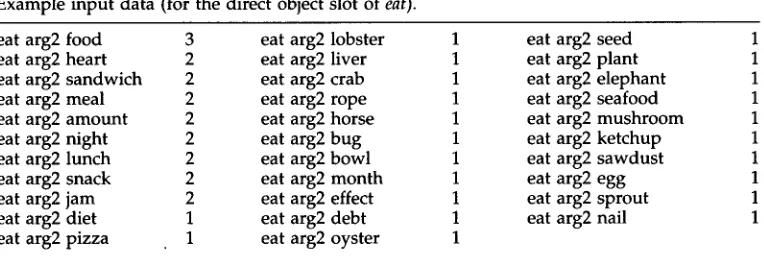
Table 6

Example input data (for the direct object slot of eat).

eat arg2 food 3 eat arg2 lobster 1 eat arg2 seed 1

eat arg2 heart 2 eat arg2 liver 1 eat arg2 plant 1

eat arg2 sandwich 2 eat arg2 crab 1 eat arg2 elephant 1

eat arg2 meal 2 eat arg2 rope 1 eat arg2 seafood 1

eat arg2 amount 2 eat arg2 horse 1 eat arg2 mushroom 1

eat arg2 night 2 eat arg2 bug 1 eat arg2 ketchup 1

eat arg2 lunch 2 eat arg2 bowl 1 eat arg2 sawdust 1

eat arg2 snack 2 eat arg2 month 1 eat arg2 egg 1

eat arg2 jam 2 eat arg2 effect 1 eat arg2 sprout 1

eat arg2 diet 1 eat arg2 debt 1 eat arg2 nail 1

eat arg2 pizza 1 eat arg2 oyster 1

applied o u r m e t h o d to generalize the slot_values. Table 6 shows some e x a m p l e triple data for the direct object slot of the verb eat.

There w e r e some extraction errors present in the data, b u t w e chose not to r e m o v e them, because in general there will always be extraction errors a n d realistic e v a l u a t i o n should leave t h e m in.

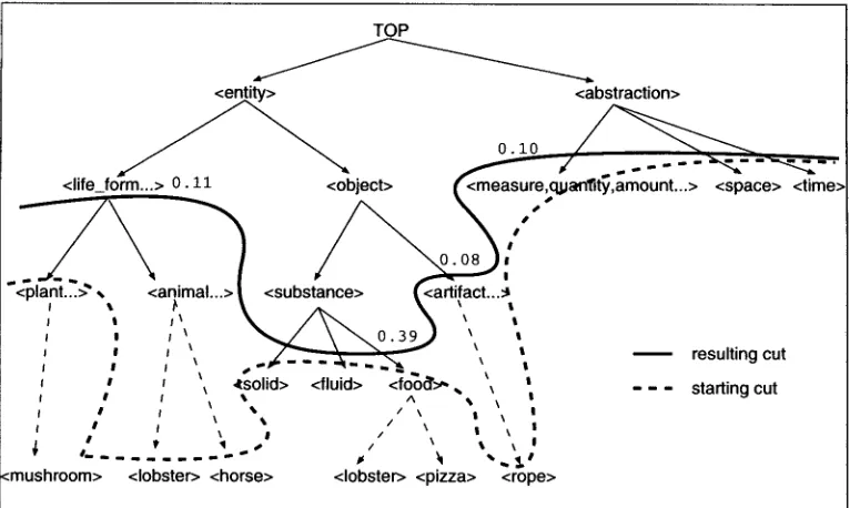
W h e n generalizing, w e used the n o u n t a x o n o m y of W o r d N e t (version 1.4) (Miller 1995) as o u r thesaurus. The n o u n t a x o n o m y of W o r d N e t has a structure of directed acyclic g r a p h (DAG), a n d its n o d e s stand for a w o r d sense (a concept) a n d often contain several w o r d s h a v i n g the same w o r d sense. W o r d N e t thus deviates from o u r notion of t h e s a u r u s - - a tree in w h i c h each leaf n o d e stands for a n o u n , each internal n o d e stands for the class of n o u n s b e l o w it, a n d a n o u n is u n i q u e l y r e p r e s e n t e d b y a leaf n o d e - - s o w e took a few measures to deal with this.

First, w e modified o u r algorithm FInd-MDL so that it can be a p p l i e d to a DAG; now, Find-MDL effectively copies each s u b g r a p h h a v i n g multiple parents (and its associated data) so that the DAG is t r a n s f o r m e d to a tree structure. N o t e that with this modification it is no longer g u a r a n t e e d that the o u t p u t m o d e l is optimal. Next, we dealt heuristically with the issue of w o r d - s e n s e a m b i g u i t y b y equally dividing the o b s e r v e d f r e q u e n c y of a n o u n b e t w e e n all the n o d e s containing that noun. Finally, w h e n an internal n o d e contained n o u n s actually occurring in the data, w e assigned the .frequencies of all the n o d e s b e l o w it to that internal n o d e , a n d excised the w h o l e subtree (subgraph) b e l o w it. The last of these measures, in effect, defines the "starting cut" of the thesaurus from w h i c h to begin generalizing. Since ( w o r d senses of) n o u n s that occur in natural language tend to concentrate in the m i d d l e of a taxonomy, the starting cut given b y this m e t h o d usually falls a r o u n d the m i d d l e of the thesaurus. 1° Figure 9 shows the starting cut a n d the resulting cut in W o r d N e t for the direct object slot of eat with respect to the data in Table 6, w h e r e / . . . / d e n o t e s a n o d e in WordNet. The starting cut consists of n o d e s / p l a n t . . . / , / f o o d / , e t c , w h i c h are the high- est n o d e s containing values of the direct object slot of eat. S i n c e / f o o d / h a s significantly higher frequencies than its n e i g h b o r s / s o l i d / a n d / f l u i d / , the generalization stops there according to MDL. In contrast, the n o d e s u n d e r / l i f e _ f o r m . . . / h a v e relatively small differences in their frequencies, a n d thus they are generalized to the n o d e / l i f e _ f o r m . . . / . The same is true of the n o d e s u n d e r /artifact/. Since / . . - a m o u n t . . . / has a m u c h

[image:15.468.35.417.71.202.2]

(16)

TOP

t ~

<abstraction>

o.i0

~ - - / . . . ~ - -~--..., -~

<life_form...> O. 11 <object> ( <measure,~:ljjafl~it~,amount...> <space> <time>

/ \ / / ",9-089 '

<plant...> % <animal...>| <substance> {<artifact...~

:

;

;,

k

\ ' ,

',

I I I ~ ~ / \ ~ 0 . 3 9 ~1 ~ t

J I I ~ _ ~ . . . . , . ~ ~ t. resulting cut

a a , ,,tsohd> <fluid> <foo~>~. ~ - - - ~t~rtinn c.==t

I I I I ~

%%

/ / \ I % I

I I \ I I

[image:16.468.52.435.44.273.2]

:mushroom> <lobster> <horse> <lobster> <pizza> <rope>

Figure 9

An example generalization, result (for the direct object slot of eat).

higher frequency than its neighbors /time/ and {space), the generalization does not go up higher. All of these results seem to agree with h u m a n intuition, indicating that our method results in an appropriate level of generalization.

Table 7 shows generalization results for the direct object slot of eat and some other arbitrarily selected verbs, where classes are sorted in descending order of their probability values. (Classes with probabilities less than 0.05 are discarded due to space limitations.)

Table 8 shows the computation time required (on a SPARC "Ultra 1" work station) to obtain the results shown in Table 7. (The computation time for loading the WordNet was excluded since it need be done only once.) Even though the noun taxonomy of WordNet is a large thesaurus containing approximately 50,000 nodes, our method still manages to efficiently generalize case slots using it. The table also shows the average number of levels generalized for each slot, namely, the average number of links between a node in the starting cut and its ancestor node in the resulting cut. (For example, the number of levels generalized f o r / p l a n t . . - / is one in Figure 9.) One can see that a significant amount of generalization is performed by our m e t h o d - - t h e resulting tree cut is about 5 levels higher than the starting cut, on the average.

4.2 Experiment 2: PP-Attachment Disambiguation

Case frame patterns obtained by our method can be used in various tasks in natural language processing. In this paper, we test its effectiveness in a structural (PP- attachment) disambiguation experiment.

(17)

Table 7

Examples of generalization results.

Class Probability Example Words

Direct Object of

eat

(food,nutrient) 0.39 pizza, egg

(life_form,organism,being,living_thing) 0.11 lobster, horse

/measure,quantity, amount,quantum) 0.10 amount

of

(artifact,article,artefact) 0.08

as if eat

rope

Direct Object of

buy

(object, inanimate-object,physical-object / 0.30 computer, painting

(asset) 0.10 stock, share

(group,grouping) 0.07 company, bank

(legal_document,legal_instrument,official_document .... ) 0.05 security, ticket Direct Object of

.fly

(entity) 0.35 airplane, flag, executive

(linear_measure,long_measure) 0.28 mile

/group,grouping) 0 . 0 8 delegation

Direct Object of

operate

/group,grouping/ 0 . 1 3 company, fleet

(act,human_action,human_activity) 0.13 flight, operation

(structure,construction/ 0.12 center

(abstraction) 0.11 service, unit

[image:17.468.38.417.80.369.2]

(possession/ 0.06 profit, earnings

Table 8

Required computation time and number of generalized levels.

Verb CPU Time (second) Average Number of Generalized Levels

eat 1.00 5.2

buy 0.66 4.6

fly 1.11 6.0

operate 0.90 5.0

Average 0.92 5.2

m a n y probabilistic m e t h o d s proposed in the literature to address the PP-attachment problem using lexical semantic knowledge which, in our view, can be classified into three types.

The first approach (Hindle a n d Rooth 1991, 1993) takes doubles of the form

(verb, prep)

a n d

(nounl, prep),

like those in Table 9, as training data to acquire semantic knowledge a n d judges the attachment sites of the prepositional phrases in quadruples of the form

(verb, nounl, prep, noun2)

e.g., (see, girl, with, telescope)--based on the acquired knowledge. Hindle a n d Rooth (1991) proposed the use of the lexical association measure calculated based on such doubles. More specifically, t h e y estimate

P(prep I verb)

and

P(prep [ noun1),

a n d calculate the so-called t-score, which is a measure of the statistical significance of the difference between

P(prep I verb)

a n d

[image:17.468.29.332.406.489.2]

(18)

Table 9

Example input data as doubles. see in

see with girl with man with

Table 10

Example input data as triples. see in park

see with telescope girl with scarf see with friend man with hat

Table 11

Example input data as quadruples and labels.

see girl in park ADV

see man with telescope ADV

see girl with scarf ADN

then the prepositional phrase is attached to

verb,

if the latter probability is significantly larger, it is attached to

nounl,

and otherwise no decision is made.

The second approach (Sekine et al. 1992; Chang, Luo, and Su 1992; Resnik 1993a; Grishman and Sterling 1994; Alshawi and Carter 1994) takes triples

(verb, prep, noun2)

and

(nounl, prep, noun2),

like those in Table 10, as training data for acquiring semantic knowledge and performs PP-attachment disambiguation on quadruples. For example, Resnik (1993a) proposes the use of the selectional association measure calculated based on such triples, as described in Section 2. More specifically, his method compares

maxclassi~noun2 A(Classi [ verb, prep)

and

maxclassi~no,m2 A(Classi I nounl,prep)

to make disambiguation decisions.

The third approach (Brill and Resnik 1994; Ratnaparkhi, Reynar, and Roukos 1994; Collins and Brooks 1995) receives quadruples

(verb, noun1, prep, noun2)

and labels indicating which w a y the PP-attachment goes, like those in Table 11, and learns a disambiguation rule for resolving PP-attachment ambiguities. For example, Brill and Resnik, (1994) propose a method they call transformation-based error-driven learning (see also Brill [1995]). Their method first learns IF-THEN type rules, where the IF parts represent conditions like

(prep

is with) and

(verb

is see), and the THEN parts represent transformations from (attach to

verb)

to (attach to

nounl),

or vice versa. The first rule is always a default decision, and all the other rules indicate transformations (changes of attachment sites) subject to various IF conditions.

We note that, for the disambiguation problem, the first two approaches are basi- cally unsupervised learning methods, in the sense that the training data are merely positive examples for both types of attachments, which could in principle be extracted from pure corpus data with no human intervention. (For example, one could just use unambiguous sentences.) The third approach, on the other hand, is a

supervised

[image:18.468.51.220.51.333.2]

(19)

Table 12

Number of different types of data. Training Data

Average number of doubles per data set 91218.1 Average number of triples per data set 91218.1 Average number of quadruples per data set 21656.6

Test Data

Average number of quadruples per data set 820.4

The generalization m e t h o d w e p r o p o s e falls into the second category, a l t h o u g h it can also be used as a c o m p o n e n t in a c o m b i n e d scheme w i t h m a n y of the a b o v e m e t h - ods (see Brill a n d Resnik [1994], Alshawi and Carter [1994]). We estimate

P(noun2 I

verb, prep)

a n d

P(noun2 I nount, prep)

from training data consisting of triples, a n d compare them: If the f o r m e r exceeds the latter (by a certain margin) w e attach it to

verb,

else if the latter exceeds the f o r m e r (by the same margin) w e attach it to

noun1.

In o u r experiments, described below, w e c o m p a r e the p e r f o r m a n c e of o u r p r o p o s e d m e t h o d , w h i c h w e refer to as MDL, against the m e t h o d s p r o p o s e d b y H i n d l e a n d Rooth (1991), Resnik (1993b), a n d Brill a n d Resnik (1994), referred to respectively as LA, SA, a n d TEL.

Data Set.

We u s e d the b r a c k e t e d c o r p u s of the Penn Treebank

(Wall Street Journal

corpus) (Marcus, Santorini, a n d Marcinkiewicz 1993) as o u r data. First w e r a n d o m l y selected one of the 26 directories of the WSJ files as the test data a n d w h a t remains as the training data. We r e p e a t e d this process 10 times a n d obtained 10 sets of data consisting of different training data a n d test data. We used these 10 data sets to c o n d u c t cross-validation as described below.

F r o m the test data in each data set, w e extracted

(verb, noun1, prep, noun2)

q u a d r u - ples using the extraction tool p r o v i d e d b y the P e n n Treebank called "tgrep." At the same time, w e obtained the a n s w e r for the PP-attachment site for each q u a d r u p l e . We did not double-check if the answers p r o v i d e d in the P e n n Treebank were actually correct or not. T h e n from the training data of each data set, w e extracted

(verb, prep)

and

(noun, prep)

doubles, a n d

(verb, prep, noun2)

a n d

(nounl,prep, noun2)

triples using tools w e d e v e l o p e d ourselves. We also extracted q u a d r u p l e s from the training data as before. We t h e n a p p l i e d 12 heuristic rules to f u r t h e r preprocess the data, w h i c h include (1) changing the inflected f o r m of a w o r d to its stem form, (2) replacing n u m e r a l s with the w o r d

number,

(3) replacing integers b e t w e e n 1,900 a n d 2,999 with the w o r d

year,

(4) replacing

co., ltd.,

etc. w i t h the w o r d s

company, limited,

etc. 11 After preprocessing there still r e m a i n e d some m i n o r errors, w h i c h w e did not r e m o v e further, d u e to the lack of a g o o d m e t h o d for d o i n g so automatically. Table 12 shows the n u m b e r of different types of data obtained b y the a b o v e process.

Experimental Procedure.

We first c o m p a r e d the accuracy a n d coverage for each of the three disambiguation m e t h o d s b a s e d on u n s u p e r v i s e d learning: MDL, SA, a n d LA.

[image:19.468.37.272.79.170.2]

(20)

0.98

0.96

0.94

0.92

0.9

0.88

0.66

0.84

0.82

0.8 0

"'-..,

"'"-,.,., "",.,

"E3, "'"', ..,

"D,. x*',

f I I {

0.2 0.4 0.6 0.8

[image:20.468.59.368.48.276.2]

coverage

Figure 10

Accuracy-coverage curves for MDL, SA, and LA.

i "MDL"

"SA" -4-- "LA" -~--

"LA.t" x •

'D,.

"~t "El

For MDL, we generalized

noun2

given

(verb, prep, noun2)

and

(nounl,prep, noun2)

triples as training data for each data set, using WordNet as the thesaurus in the same manner as in experiment 1. When disambiguating, we actually compared

P(Classl [

verb, prep)

and

P(Class2 I noun1, prep),

where

Class1

and

Class2

are classes in the out- put tree cut models dominating

noun2

in place of

P(noun2 ] verb, prep)

and

P(noun2 ]

nounl,prep). 12

We found that doing so gives a slightly better result. For SA, we employed a somewhat simplified version in which

noun2

is generalized given

(verb, prep,

noun2)

and

(nounl,prep, noun2)

triples using WordNet, and maxcl~ss,~,o,,2

A(Classi I

verb, prep)

and

maxctass,~no,n2 A(Classi l nounl, prep)

are compared for disambiguation: If the former exceeds the latter then the prepositional phrase is attached to

verb,

and otherwise to

noun1.

For LA, we estimated

P(prep ] verb)

and

P(prep ] noun1)

from the training data of each data set and compared them for disambiguation. We then eval- uated the results achieved by the three methods in terms of accuracy and coverage. Here, coverage refers to the proportion as a percentage, of the test quadruples on which the disambiguation method could make a decision, and accuracy refers to the proportion of correct decisions among them.

In Figure 10, we plot the accuracy-coverage curves for the three methods. In plot- ting these curves, the attachment site is determined by simply seeing if the difference between the appropriate measures for the two alternatives, be it probabilities or selectional association values, exceeds a threshold. For each method, the threshold was set successively to 0, 0.01, 0.02, 0.05, 0.1, 0.2, 0.5, and 0.75. When the difference between the two measures is less than a threshold, we rule that no decision can be made. These curves were obtained by averaging over the 10 data sets.

12 Recall t h a t a n o d e in W o r d N e t r e p r e s e n t s a w o r d s e n s e a n d n o t a w o r d ; noun2 c a n b e l o n g to s e v e r a l classes in t h e t h e s a u r u s . We t h u s u s e maxciassignou,2 (P(Classi [ verb, prep)) a n d

(21)

[image:21.468.29.222.87.172.2]

Table 13

Results of PP-attachment disambiguation. Coverage(%) Accuracy(%)

Default 100 56.2

MDL + Default 100 82.2

SA + Default 100 76.7

LA + Default 100 80.7

LA.t + Default 100 78.1

TEL 100 82.4

We also implemented the exact method proposed by Hindle and Rooth (1991), which makes disambiguation judgement using the t-score. Figure 10 shows the result as LA.t, where the threshold for t-score is set to 1.28 (significance level of 90 percent.) From Figure 10 we see that with respect to accuracy-coverage curves, MDL outperforms both SA and LA throughout, while SA is better than LA.

Next, we tested the method of applying a default rule after applying each method. That is, attaching

(prep, noun2)

to

verb

for the part of the test data for which no decision was made by the method in question. 13 We refer to these combined methods as MDL+Default, SA+Default, LA+Default, and LA.t+Default. Table 13 shows the results, again averaged over the 10 data sets.

Finally, we used the transformation-based error-driven learning (TEL) to acquire transformation rules for each data set and applied the obtained rules to disambiguate the test data. The average number of obtained rules for a data set was 2,752.3. Table 13 shows the disambiguation result averaged over the 10 data sets. From Table 13, we see that TEL performs the best, edging over the second place MDL+Default by a small margin, and then followed by LA+Default, and SA+Default. Below we discuss further observations concerning these results.

MDL and SA.

According to our experimental results, the accuracy and coverage of MDL appear to be somewhat better than those of SA. As Resnik (1993b) pointed

~ P(qv,r)

out, the use of selectional association Iu~ ~ seems to be appropriate for cognitive modeling. Our experiments show, however, that the generalization method currently employed by Resnik has a tendency to overfit the data. Table 14 shows example generalization results for MDL (with classes with probability less than 0.05 discarded) and SA. Note that MDL tends to select a tree cut closer to the root of the thesaurus tree. This is probably the key reason w h y MDL has a wider coverage than SA for the same degree of accuracy. One may be concerned that MDL is "overgeneralizing" here, 14 but as shown in Figure 10, its disambiguation accuracy does not seem to be degraded.

Another problem that must be dealt with concerning SA is how to remove noise (resulting, for example, from erroneous extraction) from the generalization results.

P(Clv,r)

Since SA estimates the ratio between two probability values, namely - ~ y - , the generalization result may be lead astray if one of the estimates of

P(C I v, r)

and

P(C)

is unreliable. For instance, a high estimated value f o r / d r o p , bead, pearl / at

protect against

13 Interestingly, for the entire data set it is m o r e favorable to attach (prep, noun2) to noun1, but for w h a t remains after a p p l y i n g LA and MDL, it t u r n s out to be m o r e favorable to attach (prep, noun2) to verb.

(22)

Table 14

Example generalization results for SA and MDL. Input

Verb Preposition Noun Frequency

protect against accusation 1

protect against damage 1

protect against decline 1

protect against drop 1

protect against loss 1

protect against resistance 1

protect against squall 1

protect against vagary 1

Generalization Result of MDL

Verb Preposition Noun Class Probability

protect against (act,human_action,human_activity) 0.212

protect against (phenomenon) 0.170

protect against (psychological_feature) 0.099

protect against (event) 0.097

protect against (abstraction) 0.093

Generalization Result of SA

V e r b Preposition Noun Class SA

protect against protect against protect against protect against protect against protect against protect against protect against protect against protect against protect against protect against protect against protect against protect against

(caprice,impulse,vagary, whim) 1.528

(phenomenon) 0.899

(happening,occurrence,natural_event) 0.339 (deterioration,worsening,decline,declination) 0.285 (act,human_action,human_activity) 0.260

(drop,bead,pearl) 0.202

(drop) 0.202

(descent,declivity, fall,decline,downslope) 0.188

(resistor, resistance) 0.130

(underground,resistance) 0.130

{immunity, resistance) O. 124

(resistance, opposition) 0.111

(loss,deprivation) 0.105

(loss) 0.096

(cost,price,terms,damage / 0.052

shown in Table 14 is rather odd, and is because the estimate of P(C) is unreliable (too small). This problem apparently costs SA a nonnegligible drop in disambiguation accuracy. In contrast, MDL does not suffer from this problem since a high estimated probability value is only possible with high frequency, which cannot result just from extraction errors. Consider, for example, the occurrence of car in the data shown in Figure 8, which has supposedly resulted from an erroneous extraction. The effect of this datum gets washed away, as the estimated probability for VEHICLE, to which car

has been generalized, is negligible.

[image:22.468.53.386.80.527.2]

(23)

Table 15

Some hard examples for LA.

Attached to verb Attached to noun1

acquire interest in year buy stock in trade ease restriction on export forecast sale for year make payment on million meet standard for resistance reach agreement in august show interest in session win verdict in winter

acquire interest in firm buy stock in index ease restriction on type forecast sale for venture make payment on debt meet standard for car reach agreement in principle show interest in stock win verdict in case

on their co-occurrence relation. Since both MDL and SA have pros and cons, it would be desirable to develop a methodology that combines the merits of the two methods (cf. Abe and Li [1996]).

M D L and LA. LA makes its disambiguation decision completely ignoring noun2. As

Resnik (1993b) pointed out, if we hope to improve disambiguation performance by increasing training data, we need a richer model such as those used in MDL and SA. We found that 8.8% of the quadruples in our entire test data were such that they shared the same verb, prep, noun1 but had different noun2, and their PP-attachment sites go both ways in the same data, i.e., both to verb and to noun1. Clearly, for these examples, the PP-attachment site cannot be reliably determined without knowing noun2. Table 15 shows some of these examples. (We adopted the attachment sites given in the Penn Tree Bank, without correcting apparently wrong judgements.)

M D L and TEL. We chose TEL as an example of the quadruple approach. This method

was designed specifically for the purpose of resolving PP-attachment ambiguities, and seems to perform slightly better than ours.

As we remarked earlier, however, the input data required by our method (triples) could be generated automatically from unparsed corpora making use of existing heuristic rules (Brent 1993; Smadja 1993), although for the experiments we report here we used a parsed corpus. Thus it would seem to be easier to obtain more data in the future for MDL and other methods based on unsupervised learning. Also note that our method of generalizing values of a case slot can be used for purposes other than disambiguation.

5. C o n c l u s i o n s

[image:23.468.34.295.82.198.2]

(24)

depends on the structure of the particular thesaurus used. This, however, is a problem commonly shared by any generalization method that uses a thesaurus as prior knowledge.

Appendix A: Proof of Proposition 1

Proof

For an arbitrary subtree T' of a thesaurus tree T and an arbitrary tree cut model M = (F,0) of T, let

MT,

= ( F T , , 0 T , ) denote the submodel of M that is contained in T'. Also for any sample S and any subtree T' of T, let

ST,

denote the subsample of S contained in T'. (Note that

MT = M, ST = S.)

Then define, in general for any submodel

MT,

and subsample

ST,, L(ST, [ FT,, ~T')

to be the data description length of subsample

ST,

using submodel

MT,, L(~T, [

FT,) to be the parameter description length for the submodel

MT,,

and

L'(MT,,ST,)

t o be

L(ST, I

F T ' , ~ T ' ) q-

L(~T, [ FT,).

(Note that, when calculating the parameter description length for a submodel, the sample size of the entire sample ]S] is used.)

First note that for any (sub)tree T, (sub)model

MT

= (FT, ~T) contained in T, and (sub)sample

ST

contained in T, and T's child subtrees

Ti

: i = 1 , . . . , k, we have:

k

L(ST

I PT, g ) =

L(ST,

I PT,,g,)

(17)

i=1

provided that Fz is not a single node (root node of T). This follows from the mutual disjointness of the

Ti,

and the independence of the parameters in the

Ti.

We also have, when T is a

proper

subtree of the thesaurus tree:

k

L(OT

I FT) = ~

L(OT,

I FT,). (18)

i=1

Since the number of free parameters of a model in the entire thesaurus tree equals the number of nodes in the model

minus

one due to the stochastic condition (that the probability parameters must sum to one), when T equals the entire thesaurus tree, theoretically the parameter description length for a tree cut model of T should be:

L(g I rr)

=

L r)

k

=

L(0r, I rr,)

i=1

log Isl

(19)

where ISI is the size of the entire sample. Since the second term - ~ in (19) is constant once the input sample S is fixed, for the purpose of finding a model with the minimum description length, it is irrelevant. We will thus use the identity (18) both when T is the entire tree and when it is a proper subtree. (This allows us to use the same recursive algorithm, Find-MDL, in all cases.)

It follows from (17) and (18) that the minimization of description length can be done essentially independently for each subtree. Namely, if we let

Clmin (MT, ST)

denote the minimum description length (as defined by [17] and [18]) achievable for (sub)model