A Real Options Game Involving Multiple Projects
Michi Nishihara
Abstract—The equilibrium is derived in a real options game on the basis of a multidimensional state variable. In the game, firms optimize both investment time and project choice in projects that have not been chosen by the leading competitors. We demonstrate how the equilibrium changes with the number of firms, the number of projects, and the correlation between project values. Consistent with previous findings, an increase in the number of firms and a decrease in the number of projects reduce the option value in equilibrium. A new finding suggests that the option value decreases when the numbers of both firms and projects increase by the same amount. Most interestingly, a high correlation between project values plays a positive role in mitigating preemptive competition, unlike in a monopoly. The results complement the literature of both real options games and max-options, and entails new empirical implications.
Index Terms—financial engineering, real options game, op-tions on multiple assets, optimal stopping game, max-option
I. INTRODUCTION
T
HIS paper investigates the nature of a real options game based on multiple assets. The real options approach, in which option pricing theory is applied to capital budgeting decisions, better enables us to find an optimal investment strategy and project valuation involving uncertainty and flexibility, than the conventional Net Present Value (NPV) method could (see [1]). Although the early literature on real options focuses on a monopolist’s investment, many papers have recently investigated real options games, in which game theory, combined with option pricing theory, is applied to strategic interactions among firms competing in the same market.Studies such as [2], [3], and [4] derive the equilibrium in a duopoly under the preemption game (non-zero-sum optimal stopping game1) framework, while [6], [7], and [8] derive the equilibrium in a oligopoly under the Cournot– Nash framework. The competitive equilibrium has been investigated in [1] and [9].2 The main result of these studies is that competition among firms reduces option value and accelerates the exercise of real options. This prediction has been supported by empirical tests in [12] and [13].
The previous studies on real options games assume one-dimensional Geometric Brownian Motion (GBM) to be the stochastic process (the state variable) that represents the future cash flow from a project. This is because explicit results are more appealing due to the difficulty of model calibration in many real options models; although such
Manuscript received November 17, 2010; revised December 13, 2010. This work was supported in part by KAKENHI 20710116 and 22710142.
M. Nishihara is with Graduate School of Economics, Osaka University, Osaka 560-0043, JAPAN e-mail: [email protected].
1Most of the literature of real options games models competition among
rival firms into a non-zero-sum game, while the game options literature, provoked by [5], tends to focus on a zero-sum game for a buyer and a seller. This is a main difference between real options games and game options.
2In contrast, [10] and [11] investigate the agency problem in a single firm
under the mechanism design framework.
simplification could be justified for a problem concerning a single investment project, a problem involving several projects should be modeled by a multidimensional state variable. In fact, several papers have investigated a mo-nopolist’s investment decision involving two projects using a model with a bidimensional state variable. For example, [14] investigates land development timing with an alternative land use choice and [15] investigates timing in switching methods of nuclear waste disposal. The former studies a sort of American max-option, while the latter deals with an American spread option.3
However, there have been few studies investigating a real options game based on a multidimensional state variable.4 The contribution of this paper is to derive the equilibrium in a duopoly and oligopoly, taking into account multiple projects of which value follows a multidimensional state variable. We consider the game where firms optimize both investment time and project choice among projects that have not been chosen by leading competitors. In the game, we reveal how the investment strategy and the option value in equilibrium are affected by the number of firms, the number of projects, and the correlation between project values.
In equilibrium, consistent with the main result of real options games, the option value decreases and investment takes place earlier as the number of firms increases. In addition, the option value increases with the number of projects. This result can be considered an extension of previ-ous results regarding max-options. Thus, this paper links the studies on real options games and max-options. Furthermore, this paper reveals how the equilibrium changes when the numbers of both firms and projects change; we show that the option value decreases and investment is hastened when the numbers of both firms and projects increase by the same amount. Although our model exogenously provides the number of firms and the number of projects, in the real world, the number of firms tends to increase with the number of alternatives in the market. Our result enforces the robustness of the main result of real options games.
Another new finding is that a high correlation between the values of alternatives plays a positive role in moderating competition among firms. This is in sharp contrast with the previous findings in a monopoly where, as pointed out in the max-option literature, the high correlation reduces the value of project choice and accelerates investment. In a duopoly and an oligopoly, the high correlation leads to the opposite effects of moderating the competition (positive effect) and reducing the value of project choice (negative effect). The tradeoff determines the sensitivity of the correlation with
3Refer to [16] and [17] for details of American options on multiple assets. 4Although in several papers a problem with a bidimensional state variable
respect to the option value in equilibrium. In particular, when there is an equal number of projects and firms, the high cor-relation increases the option value. This paper complements the literature of real options games by revealing the effects of the correlation and complementing the max-option literature in terms of the strategic interactions.
Although the new prediction has yet to be empirically investigated, it has the potential to account for the non-monotonicity pointed out by [13]. Their empirical work finds that, investment in medium-concentration industries takes place earlier than in not only high-concentration industries but also in low-concentration industries. Our results highlight the significance of the correlation between project values in addition to industry concentration.
Finally, we address real-world cases to which the model applies. The model could potentially account for competition in mergers and acquisitions. For instance, in the pharmaceu-tical industry, large corporations strategically acquire venture businesses that develop new drugs. In a large-scale case, a firm must choose between several targets due to budget constraint. Because many mergers and acquisitions take place by private negotiation rather than through a public bidding process, preemptive competition occurs among the acquiring firms. When a firm is preempted by its rival, it will choose an alternative venture business (plan B). The model is also closely related to strategic interactions among real estate developers. As documented in [14], a developer has several options of land uses. The value of each land use is greatly affected by land development that is done by other developers in the same area. Some developers that are preempted by its rivals are obliged to develop land for an alternative use (plan B).
II. PRELIMINARIES
Consider a firm that has an option to invest in a project. Consider two kinds of projects denoted by i = 1,2. When a firm conducts project i at time t, it receives temporary project value Xi(t).5 The investment in project i requires an irreversible capital expenditure of Ii(>0). Assume that project value Xi(t)follows a nonnegative diffusion process under the risk-neutral measure:
dXi(t) =µi(Xi(t), t)dt+σi(Xi(t), t)dBi(t), (1)
where (B1(t), B2(t)) is a bidimensional Brownian Motion
(BM) with correlation coefficient ρ. Mathematically, the model is built on the filtered probability space(Ω,F, P;Ft) generated by(B1(t), B2(t)). The setFtmeans the available information set to timet, and a firm optimizes its investment strategy under this information. Let r(> 0) and T(> 0) denote the constant risk-free rate and maturity of the option, respectively.
A. Valuation in a monopoly with a single project
As a benchmark, we consider a firm that has a monopolis-tic option to invest in a single project i. This option can be regarded as an American call option. At time t(< T) with
5This is regarded as the discounted cash flow during the lifetime of project
i.
the state variable Xi(t) =xi, the option value is equal to the value function of the optimal stopping problem:6
Vi1(xi, t) := sup τ∈TtE
xi
t [e−
r(τ−t)(X
i(τ)−Ii)1{τ≤T}], (2)
whereTt denotes the set of all stopping timesτ satisfying τ ≥t andExi
t [·] is the expectation conditional on Xi(t) = xi. Throughout the paper, the superscript and the subscript onV1
i represent the number of firms and available project(s), respectively; that is, V1
i in (2) means the value function in a monopoly with a single projecti.
We restrict our attention to a diffusion process X(t) satisfying the following assumptions:
Assumption (i) The value function Vi1(xi, t) is con-tinuous and strictly increasing with respect to xi and limxi↓0Vi1(xi, t) = 0.
Assumption (ii) There exists a finite threshold x1
i(t) such that the optimal stopping time τ1
i(t) for problem (2) is written as
τi1(t) = inf{s≥t|Xi(s)∈[x1i(s),∞)}. (3)
Define S1
1(s) := [x11(s),∞)×R+ and S21(s) := R+ ×
[x1
2(s),∞). Then, the optimal investment timeτi(t)is written as inf{s ≥ t | X(s) ∈ S1
i(s)}. The assumptions are not restrictive. Indeed, we can take a wide range of diffusion processes including a GBM, i.e., µi(Xi(t), t) = µiXi(t) andσi(Xi(t), t) =σiXi(t)whereµi(< r)andσi(>0) are constant, and a process with a mean-reverting growth rate, i.e.,µi(Xi(t), t) =η(m−Xi(t))andσi(Xi(t), t) =σiXi(t) whereη, mandσi are positive constants.
WhenX(t) follows a GBM and the maturity is infinite, V1
i (xi, t)is explicitly derived independently from timet. In fact, the option valueVi1(xi)is expressed as
Vi1(xi) =
(
xi x1
i )βi
(x1i −Ii) (0≤xi< x1i)
xi−Ii (xi≥x1i).
(4)
The constant thresholdx1
i is defined by
x1i = βi βi−1
Ii, (5)
whereβi := 1/2−µi/σ2i + √
(µi/σi2−1/2)2+ 2r/σ2i(> 1). Similarly, when X(t) follows a process with a mean-reverting process and the maturity is infinite, the option value is explicit and independent of timet. For details, refer to [1].
B. Valuation in a duopoly with a single project
This subsection considers two identical firms that compete for a single project i. Throughout the paper, we assume a winner-take-all game as follows:
Assumption (iii) A firm cannot invest in the project in which
the other firm has already invested.
Suppose time t withXi(t) = xi ≤ Ii for i = 1,2. The duopoly game is solved backward. We begin by supposing that one of the firms (the leader) has first invested at time s ∈ [t, T], and we find the optimal decision of the other (the follower). Because the follower’s opportunity to invest is removed, the follower’s value is zero. On the other hand,
6When the maturity is infinite, we have only to replace1
{τ≤T} with
the leader’s value isXi(s)−Ii at the time of investment. In the situation where neither firm has invested, firms attempt to preempt each other in order to obtain the leader’s project value if Xi(s)−Ii>0. DefineS12(s) := [I1,∞)×R+ and
S2
2(s) :=R+×[I2,∞). In equilibrium, both firms attempt
to invest at
τi2(t) := inf{s≥t|X(s)∈Si2(s)} (6)
and hence the option value becomes
Vi2(xi, t) := 0, (7)
where the superscript 2 and the subscript i represent a duopoly with a single project i. In other words, the pre-emptive competition completely removes the value of option to invest in project i.
Strictly speaking, both firms’ investment strategy at (6) proves to be a Nash equilibrium in the optimal stopping game under the assumption that if two firms choose the same timing, one of the firms is chosen as the leader with probability1/2. Most studies, including [2] and [3], are built on this assumption. Then, the equilibrium means that one of the firms invests in project i at time (6), while the other cannot undertake the project. The value of the leader, who is selected randomly, is zero because of investing too early. This is the well-known preemptive equilibrium in a real options game. For details of real options games, refer to [19].
C. Valuation in a monopoly with two projects
This subsection considers a firm that has a monopolistic option to invest in a single project between projects 1,2. The model applies not only to a case in which two projects are mutually exclusive (e.g., alternative land use) but also to a case where a firm must choose between projects due to budget constraint (e.g., large merger and acquisition trans-action). This type of option is classified as American max-options. European max-options have been studied in [20] and [21], while American max-options have been studied in [14], [16], and [17]. Although a max-option commonly has a multidimensional state variable, [22] studies a max-option that is written on a one-dimensional state variable, i.e., ρ = 1, x1 ̸= x2, and I1 ̸= I2, in order to investigate
investment timing with an alternative scale choice.
At timet(< T)withX(t) =x, the option value is equal to the value function of the optimal stopping problem as follows:
V11,2(x, t) := sup τ∈Tt
Ex t[e−
r(τ−t)max
i=1,2(Xi(τ)−Ii)
| {z }
project choice
1{τ≤T}].
(8) Recall that V1
1,2 in (8) means the value function in a
monopoly with projects1,2. The optimal stopping timeτ1 1,2
for problem (8) is written as
τ11,2(t) = inf{s≥t|X(s)∈S11,2(s)}, (9)
where the stopping regionS1
1,2(s)is defined by
S11,2(s) :={x∈R2+|V11,2(x, s) = max
i=1,2(xi−Ii)}. (10)
The stopping region S11,2(s)proves to be the union of two
disjoint convex sets corresponding to the immediate exercise
region of each project, when X(t) follows a GBM. For details, refer to [14], [17].
Let us now focus on two symmetric projects, i.e., x1 =
x2, µ1(·,·) = µ2(·,·), σ1(·,·) = σ2(·,·), and I1 = I2. In
this case, the larger the correlation coefficient ρ, the more likely it is that the project valuesX1(t)andX2(t)take close
values. The option value V1
1,2 decreases and the stopping
region S1
1,2 enlarges with ρ, because the higher ρ reduces
the value of project choice. In particular, in the case of the perfect correlation, i.e.,ρ= 1, the option valueV1
1,2 and the
investment time τ1
1,2, agree with those in a monopoly with
a single project, i.e., V1
i and τi1, respectively. The effects of the correlation will be compared in detail with that of a duopoly with two projects in Section 3.
The following section is the main contribution of the paper. Although the results can be readily extended to the case of a oligopoly with multiple projects, we present the details of a duopoly with two projects in order to avoid unnecessary confusion.
III. MAIN RESULTS
This section investigates two identical firms that compete for two projects1,2.7 Recall Assumption (iii). When one of the firms (the leader) undertakes a project, the other (the follower) is deprived of the opportunity to invest in that project. Firms attempt to preempt each other in order to gain the first-mover’s advantage in project choice. Assume that the first mover cannot invest in the remaining project. Otherwise, as in Section 2.B, both firms compete for the remaining project and gain no value from the project. Then, it follows from backward reasoning that the equilibrium value becomes zero in the situation where neither firm has invested. As mentioned in Section 1, the model can be applied to strategic interactions in acquisitions and land development.
Consider timet(< T)withXi(t) =xi≤Ii for i= 1,2. As in Section 2.B, the problem is solved backward. Supposed that one of the firms (the leader) has first invested in the better project i(s) at time s ∈ [t, T], where the function i(s)8 is defined by
i(s) := arg max
i=1,2(Xi(s)−Ii), (11)
we find the optimal response of the other firm (follower). Because the follower has the monopolistic option to invest in a single projecti̸=i(s), the option value and the optimal investment time coincide with V1
i and τi1 (cf. (2) and (3)). On the other hand, the leader’s project value is equal to maxi=1,2(Xi(s)−Ii).
Let us return to the situation where neither firm has invested. Intuitively, in equilibrium the leader’s advantage in project choice is offset by too early and inefficient investment timing. Define the region S2F
1,2(s) where the leader’s value
dominates that of the follower as follows:
S12,F2(s) := {x∈R2+|x1−I1≥V21(x2, s)} ∪{x∈R2+|x2−I2≥V11(x1, t)}.
7For simplicity, this paper concentrates on the identical firms. Although
similar (but messy) results follow from the same logic in the asymmetric case, interesting insights can be better observed in the symmetric case.
8We do not have to be concerned about the value ofi(s)whenX
1(s)−
Each firm attempts to preempt the competitor when X(s)∈ S2F
1,2(s). In addition, one of the firms is forced to invest for
X(s)∈S1
1(s)∪S21(s), if it knows that the other waits until
τ12,F2(t) := inf{s≥t|X(s)∈S12,F2(s)}. (12)
This is because for X(s) ∈ S11(s)∪S21(s) the immediate exercise yields a higher value than the option value to wait untilτ12,F2. Note that, in this equilibrium, the follower’s value
is higher than that of the leader. For details, refer to the proof of Proposition 1. Therefore, the preemptive investment regionS2
1,2(s)becomes
S12,2(s) :=S12,F2(s)∪S11(s)∪S21(s). (13)
The preemptive investment takes place at time
τ12,2(t) := inf{s≥t|X(s)∈S12,2(s)}. (14)
It is easily checked that the boundary of S2
1,2(s) can be
expressed as
∂S12,2(s)
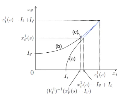
= {x∈R2+|xi≤x1i′(s)−Ii′+Ii, xi−Ii =Vi1′(xi′, s)}
| {z }
(a)
∪ {x∈R2+|xi′ ≤x1i′(s), xi′−Ii′=Vi1(xi, s)}
| {z }
(b) ∪ {x∈R2+|xi′ =x1i′(s),
| {z }
(c)
(Vi1)−1(x1i′(s)−Ii′)≤xi≤x1i′(s)−Ii′ +Ii}
| {z }
(c)
, (15)
whereiandi′(̸=i)(which may depend ons) satisfy
x1i(s)−Ii≥x1i′(s)−Ii′. (16)
Throughout the paper, we denote by i′ for i′ ̸= i. In (16), (V1
i )−1(·) (which may depend on s) denotes the inverse function for V1
[image:4.595.308.510.93.258.2]i (·, s). Note that this function is well defined by Assumption (i).
Figure 1 illustrates the preemptive investment boundary ∂S2
1,2(s). The part (a) is the region where the leader’s
investment in project i generates the same value as the follower’s option value to invest in projecti′. Similarly, the part (b) is the region where the leader’s investment in project i′ generates the same value as the follower’s option value to invest in project i. In the part (c), both firms prefer to be the follower with projectito being the leader with projecti′ due to X(s)∈/S2F
1,2(s). In equilibrium, as will be proved in
Proposition 1, one of the firms invests when X(s) hits the part (c). We see from (15) that, unlike S1
1,2 in a monopoly,
the preemptive investment regionS2
1,2 is independent of the
correlation coefficientρ.
At time t(< T) with X(t) = x, the option value of the leader is written as
V12,2(x, t) :=Ext[e−r(τ12,2(t)−t)max
i=1,2(Xi(τ 2
1,2(t))−Ii)
×1{τ2
1,2(t)≤T}]. (17)
This value is lower than that of the follower if and only if the process X(t) hits the part (c).
So far, we intuitively explain the equilibrium. More pre-cisely, we need to formulate the following optimal stopping
(a) (b)
(c)
Fig. 1. The preemptive investment boundary∂S2 1,2(s)
game for two identical firms j= 1,2. The set of actions is defined by
A(t) := {(τ, i)|τ∈ Tt, i:Fτmeasurable random variable taking values in{0,1}}.
For firm 1’s action (τ1, i1) ∈ A(t) and firm 2’s action
(τ2, i2)∈A(t), the payoff of firm1is defined by
π1(τ1, i1, τ2, i2)
:= Ext[e−r(τ1−t)(X
i1(τ1)−Ii1)
| {z }
leader’s value
1{τ1<τ2}∩{τ1≤T}
+ e−r(τ2−t)V1
i′2(Xi′2(τ2), τ2)
| {z }
follower’s value
1{τ1>τ2}∩{τ2≤T}
+e
−r(τ1−t)
2 (Xi1(τ1)−Ii1+V 1
i′2(Xi′2(τ2), τ2))
| {z }
average of leader’s and follower’s value
×1{τ1=τ2}∩{τ1≤T}].
The last term corresponds to the assumption that if two firms choose the same timing, one of the firms is chosen as the leader with probability 1/2. The payoff of firm 2 (denoted by π2(τ1, i1, τ2, i2)) is defined symmetrically.
A Nash equilibrium ( ˜τ1,i˜1,τ˜2,i˜2) ∈ A(t)×A(t) of the
stopping game satisfies both
π1( ˜τ1,i˜1,τ˜2,i˜2) = max (τ1,i1)∈A(t)
π1(τ1, i1,τ˜2,i˜2), (18)
and
π2( ˜τ1,i˜1,τ˜2,i˜2) = max (τ2,i2)∈A(t)
π2( ˜τ1,i˜1, τ2, i2). (19)
We assume that for (17) the diffusion processX(t) satis-fies9
Assumption (iv)
max
i=1,2(xi−Ii)≤V 2
1,2(x, t) (x /∈S 2 1,2(t)).
9We have not established any proof, but the assumption is satisfied in
[image:4.595.321.536.416.541.2]The following proposition shows that the pair of actions (τ2
12(t), i(τ122(t)), τ122F(t), i(τ122F(t)))∈A(t)×A(t)is a Nash
equilibrium of the stopping game, where the stopping times τ2
12(t), τ122F(t) are defined by (14),(12), and the functions
i(τ2
12(t)), i(τ122F(t))are defined by (11), respectively.
Proposition 1 (τ122(t), i(τ122(t)), τ122F(t), i(τ122F(t))) is a
Nash equilibrium of the stopping game.
Proposition 1 includes the equilibrium in a duopoly with a single project. Indeed, forxi> xi′ = 0, the equilibrium in
Proposition 1 agrees with that of Section 2.B. Accordingly, Proposition 1 extends the previous results to a more general case in which there are two opportunities to invest in. For most of the diffusion process Xi(t), a higher volatility σi leads to a higher option value Vi1 and a later investment timeτi1. If this is the case, by (15) the preemptive investment region S12,2 decreases, which leads to a higher option value
V12,2 and a later investment time τ12,2 in equilibrium. Then,
the effects of volatility σi in a duopoly remain unchanged from a monopoly.
IfX(t)follows a GBM and T =∞, we have an explicit form of the time homogeneous investment boundary ∂S21,2 by (4), (5) and (15) .
Corollary 1 Assume that T =∞, µi(Xi(t), t) =µiXi(t), andσi(Xi(t), t) =σiXi(t), whereµi(< r)andσi(>0) are constant for i = 1,2. The preemptive investment boundary is equal to
∂S21,2
=
{
xi≤x1i′−Ii′+Ii, xi−Ii= (
xi′
x1
i′ )βi′
(x1i′−Ii′) }
∪ {
xi′ ≤x1i′, xi′−Ii′ = (
xi x1
i )βi
(x1i −Ii) }
∪{xi′ =x1i′,(Vi1)−1(x1i′−Ii′)≤xi ≤x1i′−Ii′+Ii }
,
wherei(which does not depend on s) satisfies (16).
The explicit form of the investment boundary∂S2
1,2would
be useful for applications of the model. The option valueV2 1,2
(cf. (17)) can be expressed as the solution of the correspond-ing partial differential equation with the boundary ∂S2
1,2.
Then, we can computeS2
1,2 andV12,2 without difficulty.
For a general diffusion process X(t) we can show the following properties of the preemptive investment region S2
1,2(s), the timing τ12,2(t), and the option valueV12,2(x, t).
Proposition 2 The following relationships hold for all i= 1,2:
Investment region
S11,2(s)⊂S11(s)∪S21(s)⊂S21,2(s)⊂S21(s)∪S22(s), (20)
Investment timing
min(τ12(t), τ22(t))≤τ12,2(t)≤min(τ11(t), τ21(t))≤τ11,2(t), (21)
Option value
0 =Vi2(xi, t)≤V12,2(x, t)≤V 1
i (xi, t)≤V11,2(x, t). (22)
Proposition 2 reveals that the option value decreases and investment takes place earlier as the number of firms increases. This is in line with both theoretical and empirical results in real options games (e.g., [2], [6], [12], and [13]). The inequalityV2
i (xi, t)≤V12,2(x, t) means that the option
value increases with the number of projects in a duopoly. This result extends the previous result for American max-options in a monopoly (e.g., [14], [16], and [17]) into that of a duopoly. Thus, we bridge the gap between the studies on real options games and those on American max-options. In addition, Proposition 2 reveals how the equilibrium changes when the numbers of both firms and projects change. Indeed, the inequalities, V2
1,2(x, t) ≤ Vi1(x, t), τ12,2(t) ≤
min(τ1
1(t), τ21(t)), demonstrate that the option value
de-creases and investment is hastened when the numbers of both firms and projects increase by the same amount. While we exogenously provide the numbers of both firms and opportu-nities, in reality, the number of firms tends to increase with the number of opportunities. Taking this into consideration, our new result can be positioned as an extension of the previous works into a more practical setting.
We now consider two symmetric projects, i.e.,x1 =x2,
µ1(·,·) = µ2(·,·), σ1(·,·) = σ2(·,·), and I1 = I2. In the
sensitivity analysis, we focus on the correlation coefficientρ because the previous strategic models with a one-dimensional state variable cannot reveal the comparative statics with re-spect toρ. For instance, [23] investigates a duopoly with two projects, but they cannot capture the effects of the correlation between project values due to the one-dimensional model. By Proposition 2, we can easily show the following corollary.
Corollary 2 Consider the symmetric projectsi= 1,2. The following equalities hold for the correlation coefficientρ:
max ρ∈[−1,1]V
2
1,2(x, t) =Vi1(xi, t) = min ρ∈[−1,1]V
1
1,2(x, t), (23)
whereρ= 1maximizesV12,2(x, t)and minimizesV11,2(x, t).
Corollary 2 highlights a difference between max-options in a monopoly and in a duopoly. In a monopoly, as is noted in the max-option literature, the high correlation reduces the value of project choice. Conversely, the high correlation in a duopoly plays a positive role in mitigating preemptive com-petition and increasing the option value. Note that the high correlation reduces the first-mover’s advantage in project choice. This finding complements the max-option literature by demonstrating the positive effect of the high correlation in combination with strategic interactions.
on the numbers of both firms and projects but also on the correlation between project values.
We compare the option value V2
1,2 in a duopoly with that
of American min-option in a monopoly. The exercise of the min-option at timeτ, unlike the max-option, yields the payoff mini=1,2(Xi(τ)−Ii). At timet(≤T)withXi(t) =xi, the option value of American min-option is the value function of the optimal stopping problem as follows:
Vmin1 (x, t) := sup τ∈Tt
Ex t[e−
r(τ−t)min
i=1,2(Xi(τ)−Ii)1{τ≤T}].
(24) This type of option is investigated in [24] and [17]. We can show that V1
min(x, t) ≤ V12,2(x, t), where the equality
holds for the symmetric projects withρ= 1, as follows. Let Smin1 (s) be the stopping region for problem (24). Consider the boundary of S12,2(s)∪Smin1 (s). For x ∈ ∂S
2 1,2(s)\
Smin1 (s), V12,2(x, s) is either V11(x, s) or V21(x, s) which
is lager than V1
min(x, s). For x ∈ ∂Smin1 (s) \ S12,2(s),
V1
min(x, s) is equal to mini=1,2(xi−Ii) which is smaller than V2
1,2(x, s) under Assumption (iv). Then, we have
V1
min(x, s)≤V12,2(x, s)on the boundary. For the hitting time
˜
τ to the boundary, we have
Vmin1 (x, t) = Ext[e−r(˜τ−t)Vmin1 (X(˜τ),τ)1˜ {τ˜≤T}]
≤ Ex t[e−
r(˜τ−t)V2
1,2(X(˜τ),τ)1˜ {˜τ≤T}] = V12,2(x, t).
Then, the option value V2
1,2 in a duopoly is higher than the
min-option valueV1
min.
REFERENCES
[1] A. Dixit and R. Pindyck, Investment Under Uncertainty. Princeton: Princeton University Press, 1994.
[2] S. Grenadier, “The strategic exercise of options: development cascades and overbuilding in real estate markets,” Journal of Finance, vol. 51, pp. 1653–1679, 1996.
[3] H. Weeds, “Strategic delay in a real options model of R&D competi-tion,” Review of Economic Studies, vol. 69, pp. 729–747, 2002. [4] K. Huisman and P. Kort, “Strategic investment in technological
in-novations,” European Journal of Operational Research, vol. 144, pp. 209–223, 2003.
[5] Y. Kifer, “Game options,” Finance and Stochastics, vol. 4, pp. 443– 463, 2000.
[6] S. Grenadier, “Option exercise games: an application to the equilibrium investment strategies of firms,” Review of Financial Studies, vol. 15, pp. 691–721, 2002.
[7] B. Lambrecht and W. Perraudin, “Real options and preemption under incomplete information,” Journal of Economic Dynamics and Control, vol. 27, pp. 619–643, 2003.
[8] J. Jou and T. Lee, “Irreversible investment financing and bankruptcy decisions in an oligopoly,” Journal of Financial and Quantitative
Analysis, vol. 43, pp. 769–786, 2008.
[9] A. Zhdanov, “Competitive equilibrium with debt,” Journal of Financial
and Quantitative Analysis, vol. 42, pp. 709–734, 2007.
[10] S. Grenadier and N. Wang, “Investment timing, agency, and informa-tion,” Journal of Financial Economics, vol. 75, pp. 493–533, 2005. [11] T. Shibata and M. Nishihara, “Dynamic investment and capital
structure under manager-shareholder conflict,” Journal of Economic
Dynamics and Control, vol. 34, pp. 158–178, 2010.
[12] E. Schwartz and W. Torous, “Commercial office space: Testing the implications of real options models with competitive interactions,”
Real Estate Economics, vol. 35, pp. 1–20, 2007.
[13] E. Akdo˘gu and P. MacKay, “Investment and competition,” Journal of
Financial and Quantitative Analysis, vol. 43, pp. 299–330, 2008.
[14] D. Geltner, T. Riddiough, and S. Stojanovic, “Insights on the effect of land use choice: The perpetual option on the best of two underlying assets,” Journal of Urban Economics, vol. 39, pp. 20–50, 1996. [15] H. Louberg´e, S. Villeneuve, and M. Chesney, “Long-term risk
manage-ment of nuclear waste: a real options approach,” Journal of Economic
Dynamics and Control, vol. 27, pp. 157–180, 2002.
[16] M. Broadie and J. Detemple, “The valuation of american options on multiple assets,” Mathematical Finance, vol. 7, pp. 241–286, 1997. [17] J. Detemple, American-Style Derivatives valuation and computation.
London: Chapman & Hall/CRC, 2006.
[18] K. Miltersen and E. Schwartz, “R&D investments with competitive interactions,” Review of Finance, vol. 8, pp. 355–401, 2004. [19] K. Huisman, Technology Investment: A Game Theoretic Real Options
Approach. Boston: Kluwer Academic Publishers, 2001.
[20] R. Stulz, “Options on the minimum or the maximum of two risky assets: Analysis and applications,” Journal of Financial Economics, vol. 10, pp. 161–185, 1982.
[21] H. Johnson, “Options on the maximum or the minimum of several assets,” Journal of Financial and Quantitative Analysis, vol. 22, pp. 227–283, 1987.
[22] J. D´ecamps, T. Mariotti, and S. Villeneuve, “Irreversible investment in alternative projects,” Economic Theory, vol. 28, pp. 425–448, 2006. [23] M. Nishihara and A. Ohyama, “R&D competition in alternative
technologies: A real options approach,” Journal of the Operations
Research Society of Japan, vol. 51, pp. 55–80, 2008.
[24] S. Villeneuve, “Exercise regions of american options on several assets,”