Optimal Data Split Methodology for Model Validation

Optimal Data Split Methodology for Model

Validation

Rebecca Morrison, Corey Bryant, Gabriel Terejanu, Kenji Miki, Serge Prudhomme

Abstract—The decision to incorporate cross-validation into validation processes of mathematical models raises an immedi-ate question – how should one partition the data into calibration and validation sets? We answer this question systematically: we present an algorithm to find the optimal partition of the data subject to certain constraints. While doing this, we address two critical issues: 1) that the model be evaluated with respect to predictions of a given quantity of interest and its ability to reproduce the data, and 2) that the model be highly challenged by the validation set, assuming it is properly informed by the calibration set. This framework also relies on the interaction between the experimentalist and/or modeler, who understand the physical system and the limitations of the model; the decision-maker, who understands and can quantify the cost of model failure; and the computational scientists, who strive to determine if the model satisfies both the modeler’s and decision-maker’s requirements. We also note that our framework is quite general, and may be applied to a wide range of problems. Here, we illustrate it through a specific example involving a data reduction model for an ICCD camera from a shock-tube experiment located at the NASA Ames Research Center (ARC).

Index Terms—Model validation, quantity of interest, Bayesian inference

I. INTRODUCTION

Model validation to assess the credibility of a given model is becoming a necessary activity when making critical decisions based on the results of computer modeling and sim-ulations. As stated in [1], validation requires that the model accurately capture the critical behavior of the system(s), and that uncertainties due to random effects be quantified and correctly propagated through the model.

There are various approaches to model validation; here we explore a procedure based on cross-validation. First, one partitions the data into two sets: the calibration (or training) set and thevalidationset. Next, the calibration set is used to calibrate the model. Then the calibrated model produces a set of predicted values to be compared with the validation set. A small discrepancy between predicted values and the validation set improves the credibility of the model while a large discrepancy may invalidate the model. We will present a general framework based on these principles that incorporates our particular goals along with a detailed cross-validation algorithm.

More specifically, we examine situations in which we want to predict values for which experimental data is not available, referred to here as the prediction scenario. Experiments for this scenario may be impractical or even impossible. Still,

Manuscript received June 30, 2011; revised August 13, 2011. This material is based upon work supported by the Department of Energy [National Nuclear Security Administration] under Award Number [DE-FC52-08NA28615].

All authors are located at the Institute for Computational Engineering and Sciences, The University of Texas at Austin; Austin, TX, 78712 e-mail:

{rebeccam, cbryant, terejanu, kenji, serge}@ices.utexas.edu.

as a computational scientist, one wants to predict a certain quantity of interest (QoI) at this scenario and assess the quality of this prediction. Often, the only experimental data available comes from legacy experiments and may be incom-plete. Furthermore, this QoI is seldom directly observable from the system, but requires some additional modeling.

Numerous examples of this situation exist. Computational models aimed at predicting the reentry of space vehicles are one such example. Some characteristics of the system can be recreated in sophisticated wind tunnels, but experiments are expensive and may be unreliable. Another example is the maintenance of nuclear stockpiles. Since experiments to assess environmental impact in case of failure are banned, predictive models must be used.

Babuˇska et al. present a systematic approach to assess predictions of this type using Bayesian inference and what they call a validation pyramid [2]. Scenarios of varying complexity are available that suggest an obvious hierarchy on which to validate the model. In their calibration phase, Bayesian updating is used to condition the model on the observations available at lower levels of the pyramid. The model’s predictive ability is then assessed by further condi-tioning using the validation data at the higher levels. One advantage of their approach is that the prediction metric is directly related to the QoI. This feature is maintained in our work.

In the work described above, the authors employ a single split of the data into calibration and validation scenarios. While they argue that this partition of the data is made clear by the experimental set-up and validation pyramid, it is often the case that all experiments provide an equal amount of information regarding the QoI. To avoid a subjective choice of the calibration set, we determine the set by a more rigorous and quantitative process.

To do this, we propose a cross-validation inspired method-ology to partition the data into calibration and validation sets. In contrast to previous works, we do not immediately choose a single partition as above, nor do we use averages or estimators over multiple splits (see [3]–[5] and references therein). Instead, our approach first considers all possible ways to split the data into disjoint calibration and validation sets which satisfy a chosen set size. Then, by analyzing several splits, we methodically choose what we term the “optimal” split. Once the optimal split is found, we are then able to judge the validity of the model, and whether or not it should be used for predictive purposes.

posterior distribution for the model parameters.

Second, we address a fundamental issue of validation. We can never fully validate a model; instead, we can only try to invalidate it. Because of this, when we choose a validation set with which to test the model, it should be the most challenging possible. In other words, we demand that the model perform well on even the most challenging of validation sets; otherwise, we cannot be confident in its prediction of the QoI.

With these concepts in mind, we propose that the optimal split satisfy the following desiderata:

(I) The model is sufficiently informed by the calibration set (and is thus able to reproduce the data).

(II) The validation set challenges the model as much as possible with respect to the quantity of interest. Using the optimal partition, we are then able to answer whether the model should be used for prediction.

In the current work, we apply our framework to a data reduction model which converts photon counts received by an ICCD camera to radiative intensities [6]. We chose this as an appropriate application because the resulting intensities are later used to make higher-level decisions. Thus, the validity of the model should be thoroughly tested before the model is deemed reliable. Moreover, the uncertainty in such a model should be explicitly evaluated, as possible errors may be propagated through to other predicted quantities.

The paper is organized as follows. In section II, the general framework is detailed step by step. A concise algorithm is provided. In section III, the approach is applied to the data reduction model. Finally, in section IV, short-comings and future work are discussed.

II. VALIDATIONFRAMEWORK

(θ) (θ)

v (D )

π π(D )c

(θ) (θ)

c

v

σ

c

σ

π_v π

Estimate Feedback Control

p

v c

S

S

S No

Data Data

Model with

Re−Calibrated Parameter(s)

Model with

Calibrated Parameter(s)

Validation

v

v

Scenario Validation Scenario Calibration

Sensitivity/ Uncertainty Scenario Prediction

using QoI

Q

Quantification

Yes

Decision Calibration

c γ

D( Q Q ) <, c

Q

Invalid Confidence

Increased is

Model not Invalid Model

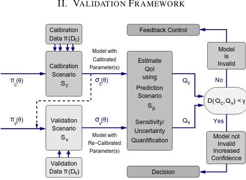
Fig. 1. The calibration and validation cycle

Figure 1 demonstrates the previously described framework [2], which applies when the quantity of interest is only available as a prediction through the computational model, not through direct observation. There, Bayesian updating is performed on a calibration set, and then a prediction of the QoI is made using the updated model. A subsequent update is performed using a validation set followed by an additional prediction with the newly updated model. Finally, the two predictions are compared to assess the model’s predictive capabilities.

A. Prediction metric

The QoI driven model assessment developed in [2] re-quires a metric comparing predictions of the QoI obtained from the calibration and validation sets. In many instances the QoI is determined by a decision-maker, who may not be the computational scientist performing the analysis. Con-sequently, they must work together to develop a suitable metric for the QoI, as well as a tolerance, which quantifies how consistent the predictions must be (note that we cannot measure accuracy of the predictions because we have no true value). Ideally this metric would measure in the units of the QoI, or provide a relative error, allowing for easy interpretation by decision-makers. Examples of such metrics include absolute error measures and percent error based on a nominal value.

In the following sections of the paper we will denote the metric used to measure the predictive performance of the model byMQ, highlighting the fact that it is determined by the QoI. Likewise, we will denote the threshold, or tolerance, byM_Q∗. We stress that generality is maintained since the rest of the procedure discussed below is flexible to the particular choice of metric and threshold. What we do require is that the choice of metric be appropriate for the application at hand. For instance, when using Bayesian inference we require that the metric be compatible with probabilistic inputs, since predictions are provided as probability or cumulative density functions of the QoI.

B. Data reproduction

As discussed briefly in the introduction, one must also ensure that the model is capable of reproducing the observed data. This evaluation has been overlooked, or at least not emphasized, in previous works [2], [6]. Such an evaluation provides confidence that the model and data provided are mutually suitable. Verifying the model’s reproducibility of the observables demonstrates that the parameters of the model are adequately informed through the inverse problem. As in the case of the prediction metric, establishing a performance criterion may require further knowledge of the physical system. The analyst is likely not an expert in the system being modeled and should solicit a modeler’s, or experimentalist’s, assistance in developing a performance metric and tolerance. Doing so will certify that the correct aspects of the system are being captured sufficiently by the model.

We use a similar notation as for the prediction metric. Let MD andM_D∗ denote the data reproduction metric and threshold respectively. We note again that these choices are defined based on the model being considered and are not specific to the framework we propose.

C. Choice of calibration size

With that being said, we do recognize that the particular choice could impact the final conclusion and must be made with care. Of particular concern is providing enough data so that all parameters of the model are sufficiently informed by the inverse problem. If the model were to fail with respect to the data metric, the issue may not be the model itself but too small a calibration set size. In this case one should perform further analysis to determine the source of this discrepancy and increase the calibration set size if necessary.

Given N observations, we denote the size of the calibra-tion set by NC and the size of the validation set by NV. That is,

NC+NV =N. (1)

Note that it could be the case that each of theN observations in fact represents a set of observations, if, for instance, repeated experimental measurements are taken at the same conditions.

We do not perform our analysis on a single partitioning of the data but instead consider all possible partitions of the data respecting (1). The reason for this approach is two-fold. First, it reduces the sensitivity of the final outcome to any particular set of data. Since each data point is equivalent under partitioning, we do not bias the groupings in any subjective way (once we have chosen the calibration set size). Second, we envision an application where it is unclear which experiments relate more closely to the QoI scenario. Considering all admissible partitions can provide insight as to which observations are most influential with respect to the QoI. As an example, consider a case of resonance where the QoI is associated with the resonant behavior of the system. Without knowing a priori the resonance frequency of the system, one cannot say which frequencies will be important for capturing the resonant behavior.

However, the drawback of this approach is evident: we must consider the model performance for all partitions of the data. This yields a combinatorially large number of partitions, whose exact number is given by the binomial formula:

P =

N NC

= N!

NC!NV!. (2)

We will denote these partitions, or splits, by {sk}, where k= 1,2, . . . , P. The computational impact of this becomes even more significant while performing the next step of the procedure.

D. Inversion for model parameters

For each admissible partition of the data, we solve an inverse problem using the calibration set, of size NC, as input data. It is not hard to see why solvingP inverse prob-lems may be difficult, or even impossible, for complicated models. This is an area for improvement; approximations and alternative approaches to reduce the number of inverse problems will be the subject of future work.

As discussed previously, we treat the inverse problem in a probabilistic setting, using Bayesian updating to incorporate the calibration data. As a result we obtain distributions of model parameters, and these in turn yield distributions for the predicted quantities. At this point it becomes clear that the definition of the metrics will depend on how the inverse problems are solved. Note, of course, that a deterministic approach could also be used.

E. Computation of the metrics

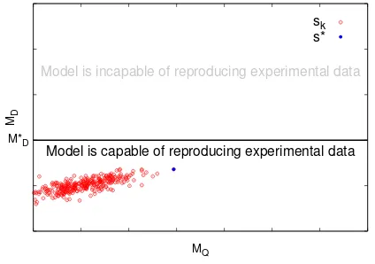
With the solutions obtained from the inverse problems we are now able to evaluate the model’s performance. For each calibration set, we compute the metrics as detailed above. One can then visualize the data on a Cartesian grid where the x and y axes correspond to the metrics MQ and MD, respectively, and each point corresponds to a single partition of the data into a calibration and validation set (figure 2).

MD

MQ

s_k

Fig. 2. Metrics computed for each data splitsk

F. Optimal partition

We attempt to invalidate the model using the optimal split determined by (I) and (II).

For (I), performance in replicating the observables is measured using the data metricMD. Thus we only consider splits,sk, of the data that satisfy

MD(sk)< MD∗.

If no points lie below this threshold, the model’s ability of reproducing the observed data is unsatisfactory, and one must change or improve the model, or the data, or perhaps both.

Next, to satisfy (II), we select the partition s∗ which maximizes the prediction metric,

s∗= argmax

sk, MD(sk)<MD∗

MQ(sk). (3)

The optimal partition for the results shown above is high-lighted in figure 3.

M*_D

MD

M_Q

Model is incapable of reproducing experimental data

s_k s*

Model is capable of reproducing experimental data

G. Comparison ofs∗ withM_Q∗

Finally we are able to assess the model’s ability to predict the QoI. After identifying the optimal partition we compare the model’s performance, in this “worst case” scenario, against the thresholdM_Q∗.

If s∗ fails to satisfy the threshold then we conclude that the model is invalid, given the observations available, and should not be used to make predictions for the QoI. Figure

M*_D

M*_Q

MD

M_Q

Model is incapable of reproducing experimental data

s_k s*

Model is not invalidated

Model is incapable of predicting QoI

Fig. 4. Comparison ofs∗withM_Q∗

4 shows an example of exactly this case.

If s∗ does not violate the tolerance set by the decision-maker we can only conclude that the model is not invalidated given the observations we have. This does not guarantee that the model is valid, only that we cannot demonstrate otherwise. This outcome warrants further observations to continue challenging the model. The process to obtain these additional experimental results may be supplemented by performing optimal experimental design [7]. If, however, we cannot obtain more data, then the process is complete, and we conclude that the model has not been invalidated.

H. Algorithm

The general algorithm can be summarized in 8 steps:

1. elicit the data metric and threshold,MDandM_D∗, from the modeler and/or experimentalist

2. elicit the QoI metric and threshold,MQ andM_Q∗, from the decision-maker

3. givenN, choose the calibration set size,NC, such that

NC+NV =N

4. generate all possible partitions of the data {sk}P k=1, where

P =

_N

NC

= N!

NC!NV!

5. solve P inverse problems for splits{sk}P k=1

6. for each partitionsk, computeMD(sk)andMQ(sk) 7. find optimal split

s∗= argmax

sk, MD(sk)<MD∗

MQ(sk)

8. compareMQ(s∗)withMQ∗

Once more we stress that the procedure described above is extremely general. This is an advantage of the approach and allows for its application to a wide range of problems. Specifics will be discussed for one application below.

III. APPLICATION TO THE DATA REDUCTION MODEL

We now turn to a specific implementation of the proposed algorithm. A data reduction model is chosen for analysis. Since higher level models require predictions obtained from this data reduction model, it is critical that we accurately assess the quality of its predictions. Moreover, we must consider all partitions of the data because the model is significantly influenced by the data.

The inverse problem of calibrating the model parameters from the measurement data is solved using Markov chain Monte Carlo simulations. In our simulations, samples from the posterior distribution are obtained using the statistical library QUESO [8] equipped with the Hybrid Gibbs Tran-sitional Markov Chain Monte Carlo method proposed by Cheung and Beck [9].

First, we briefly describe the experimental set-up, the model in question, and the quantity of interest. Next, we describe the application of the algorithm and present the results.

A. The ICCD camera

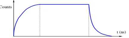
The example problem comes from a shock-tube experi-ment in which an ICCD camera measures photon counts [6]. As the opening time, or gate width, of the camera increases, so does the photon count. For sufficiently large gate widths, this behavior is linear and simple to model. However, at very small gate widths, below the linear regime of the instrument, the behavior becomes complicated and nonlinear. Figure 5 shows a diagram of this behavior. It is in this nonlinear region where we wish to predict the photon count.

t (ns) Counts

Fig. 5. Photon count vs. time for a small gate width in the ICCD camera

The raw data are photon counts received by the camera at eleven different gate widths ranging from 0.5 to 10 micro-seconds. Given the photon count,N∆t,computing the quantity of interest is a simple post-processing step. The reciprocityρis defined as

ρ(∆t) =

_N10

10

/

_N∆t

∆t

, (4)

and the QoI isρ(0.1). A data reduction model for the photon count as a function of gate width,N∆t, is required because we do not have the dataN0.1.

If we only wished to predict the photon count in the linear regime of the instrument, we could simply use:

But in order to account for the nonlinearity encountered at very small gate widths, several new parameters are intro-duced into the model:

N∆t=β(∆t+δ)−β

(α1−α2)

(α1α2) (1−e

−α1(∆t+δ)_{). (6)}

Here,βdescribes the linear term as before, andδis a correc-tion to the gate width ∆t, in case it is reported incorrectly. Also,α1andα2allow for differing opening and closing rates of the camera, respectively. These four parameters must later be calibrated through the inverse problem.

B. Application of the algorithm

Now we apply the proposed algorithm to the example problem. The steps are as follows:

1. As mentioned above, predictions of the quantity of in-terest result in cumulative distribution functions (CDFs) in the units of the QoI. Thus, we compare the maximum horizontal distance between the CDFs, with some cutoff at the tails [2]. In general, for two CDFsF andG, we define:

MQ= max

u∈(

2,1−

2)

|xF,u−xG,u|

where xF,u= min{x∈R;F(x)≥u}.

Here,F is the posterior CDF using the calibration data, Gis the posterior CDF using all the data (including the validation data), and is a parameter between 0 and 1 controlling the amount of cut-off of the tails. See figure 6.

Using this metric, the tolerance for the quantity of interest is set. In this example, the threshold isM∗

Q= 2, which corresponds to the rather large percent error of about 100%.

Fig. 6. the metric for the QoI

2. The model’s performance with respect to the data is characterized using a normalized difference between the true observations and the corresponding predicted values:

MD=E q

(X−D)T _diag(D)−1 _(X−D)

whereD is a vector of all the data, andX is a vector of the predicted values corresponding point-wise toD. Note that the entries of X are the predicted values of the observables using the calibrated model (on just the calibration set), but for all values of gate widths (including those corresponding to both calibration and validation sets).

Using the above as the data metric, the tolerance M_D∗ is set to 0.2, which yields an average relative error of 20%.

3. Given 11 gate widths, we choose calibration set size NC = 7, leaving the validation set size as NV = 4. In fact, as described earlier, multiple data points are provided for each of the gate widths. However, these points are not considered individually during the par-tioning process, but are kept together as a single unit. 4. We generate all possible data sets for calibration:

₁₁

7

= 330.

5. We solve these 330 inverse problems. Again, this is done probabilistically using uniform priors on all parameters and Bayesian updating.

6. We computeMQ andMDfor each of the 330 splits of the data. Results are shown in figure 7.

7. We find all points which satisfy MD(sk) < M_D∗. In this example, all points satisfy this requirement. Next, we find

s∗= argmax

sk, MD(sk)<MD∗

MQ(sk).

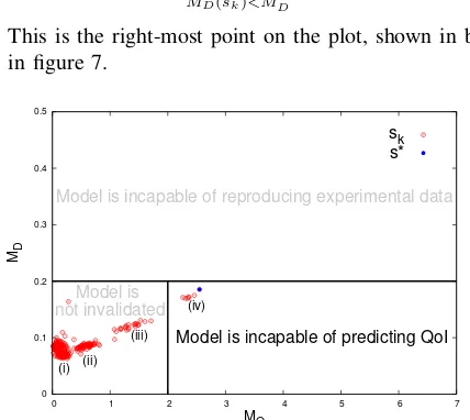
This is the right-most point on the plot, shown in blue in figure 7.

0 0.1 0.2 0.3 0.4 0.5

0 1 2 3 4 5 6 7

MD

M_Q

Model is incapable of reproducing experimental data

s_k s*

Model is not invalidated

Model is incapable of predicting QoI

(i) (ii)

(iii) (iv)

Fig. 7. Results as described in step 7.

8. We compareMQ(s∗)withMQ∗. SinceMQ(s∗)> MQ∗, then we must conclude that the model is incapable of predicting the QoI, and has thus been invalidated.

C. Analysis of results

Looking at figure 7, we see that the points, representing splits, are grouped into four regions. First, we note that s∗ belongs to group (iv), and as group number increases, the size of the group decreases. Now let us examine whys∗ is the most challenging of the splits and why these groups have formed.

First, recall that the data we received was N∆t, where

The calibration set fors∗ is missing0.5,0.6,0.7,0.8. The other points in group (iv) are those whose calibration set is missing0.5,0.6,0.7, but at least contains0.8, making them slightly less challenging than s∗. Next, group (iii) contains those splits whose calibration set is missing 0.5 and 0.6. Similarly, in group (ii), we see all the splits whose calibration set is missing 0.5. Finally, in group (i), the calibration sets contain0.5, and some collection of the remaining points.

The grouping of the data suggests a possible way to decrease the number of inverse problems performed. By finding representatives of the groups, we could search for the optimal split without analyzing every one. Moreover, in the case that the model is not invalidated, understanding these groups could be helpful when planning further experiments, perhaps through experimental design.

IV. CONCLUSION

Computationally, our approach is prohibitively expensive and requires significant improvement. Methods to reduce the number of inverse problems required are being investigated. Among them is the use of mutual information to group observations into sets containing similar data. These larger sets then require fewer inverse problems.

With experimental design one may be able to choose where to perform subsequent experiments that will challenge the model further, finding a new optimal split. This newly determined split could render the model invalid, or provide increased confidence in the model’s predictive capability.

This paper has proposed and demonstrated a systematic framework for assessing a model’s predictive performance with respect to a particular quantity of interest. Extending the work of Babuˇska et al., the ability of the model to reproduce experimental observations was also evaluated.

A data reduction model was examined using our frame-work and ultimately deemed invalid. While the model was capable of reproducing the observations at higher gate widths, it failed based on its performance in predicting the quantity of interest. The analysis was carried out on all partitions of the data respecting a chosen size constraint. This allowed for the determination of an optimal set satisfying calibration (I) and validation (II) requirements.

REFERENCES

[1] R. Hills, M. Pilch, K. Dowding, J. Red-horse, T. Paez, I. Babuˇska, and R. Tempone, “Validation challenge workshop,”Computer Methods in

Applied Mechanics and Engineering, vol. 197, no. 29 - 32, pp. 2375

– 2380, 2008.

[2] I. Babuˇska, F. Nobile, and R. Tempone, “A systematic approach to model validation based on bayesian updates and prediction related rejection criteria,” Computer Methods in Applied Mechanics and

Engineering, vol. 197, no. 29-32, pp. 2517 – 2539, 2008, Validation

Challenge Workshop.

[3] A. Vehtari and J. Lampien, “Bayesian model assessment and compar-ison using cross-validation predictive densities,”Neural Computation, vol. 14, pp. 2439 – 2468, 2002.

[4] S. Arlot and A. Celisse, “A survey of cross-validation procedures for model selection,”Statistics Surveys, vol. 4, pp. 40 – 79, 2010. [5] F. Alqallaf and P. Gustafson, “On cross-validation of bayesian models,”

The Canadian Journal of Statistics, vol. 29, no. 2, pp. 333–340, 2001.

[6] M. Panesi, K. Miki, and S. Prudhomme, “On the validation of a data reduction model with application to shock tube experiments,”

Computer Methods in Applied Mechanics and Engineering, 2011,

under review.

[7] G. Terejanu, R. R. Upadhyay, and K. Miki, “Bayesian Experimental Design for the Active Nitridation of Graphite by Atomic Nitrogen,”

Experimental Thermal and Fluid Science, 2011, under review.

[8] E. E. Prudencio and K. W. Schulz, “The Parallel C++ Statistical Library ‘QUESO’: Quantification of Uncertainty for Estimation, Sim-ulation and Optimization,”Submitted to IEEE IPDPS, 2011. [9] S. H. Cheung and J. L. Beck, “New bayesian updating methodology

for model validation and robust predictions of a target system based on hierarchical subsystem tests.”Computer Methods in Applied

Me-chanics and Engineering, 2009, accepted for publication.

[10] J. Larsen and C. Goutte, “On optimal data split for generalization estimation and model selection,” in Neural Networks for Signal Processing IX, 1999. Proceedings of the 1999 IEEE Signal Processing