Unsupervised Learning of Morphology

(1)

Unsupervised Learning of Morphology

Harald Hammarström

∗

Radboud Universiteit and Max Planck Institute for Evolutionary Anthropology

Lars Borin

∗∗

University of Gothenburg

This article surveys work on Unsupervised Learning of Morphology. We define Unsupervised Learning of Morphology as the problem of inducing a description (of some kind, even if only morpheme segmentation) of how orthographic words are built up given only raw text data of a language. We briefly go through the history and motivation of this problem. Next, over 200 items of work are listed with a brief characterization, and the most important ideas in the field are critically discussed. We summarize the achievements so far and give pointers for future developments.

1. Introduction

Morphologyis understood here in its usual sense in linguistics, namely, as referring to (the linguistic study and description of) the internal structure of words. More speciﬁ-cally, we understand morphology following Haspelmath (2002, page 2) as “the study of systematic covariation in the form and meaning of words.” For our purposes, we assume that we have a way of identifying the text words of a language, ignoring the fact that the termwordhas eluded exhaustive cross-linguistic deﬁnition. Similarly, we assume a number of commonly made distinctions in linguistic morphology, whose basic import is indisputable, but where there is an ongoing discussion on exactly where to draw the boundaries with respect to particular phenomena in individual languages.

Generally, a distinction is made betweeninflectional morphologyandword forma-tion. Inflectional morphology deals with the various realizations of the “same” lexical word, depending on the particular syntactic context in which the word appears. Typical examples of inflection are verbs agreeing with one or more of their arguments in the clause, or nouns inflected in particular case forms in order to show their syntactic rela-tion to other words in the phrase or clause, for example, showing which verb argument they express. Word formation deals with the creation of new lexical words from existing

∗Centre for Language Studies, Radboud Universiteit, Postbus 9103, 6500 HD Nijmegen, The Netherlands/ Department of Linguistics, Max Planck Institute for Evolutionary Anthropology, Deutscher Platz 6, 04103 Leipzig, Germany. E-mail:h.hammarstrom@let.ru.nl.

∗∗Språkbanken, Department of Swedish Language, University of Gothenburg, Box 200, SE-405 30 Göteborg, Sweden. E-mail:lars.borin@svenska.gu.se.

(2)

ones, for example, agent nouns from verbs. If the same kinds of mechanisms are used as in inﬂectional morphology (i.e., the resulting word is derived out of only one existing word), linguists talk about derivational morphology. If two or more existing lexical words are combined in order to make up a new word, the terms compounding or

incorporationare used, depending on the categories of the words involved.

There is a fairly wide array of formal means available cross-linguistically for ex-pressing inflectional and derivational categories in languages. Most commonly, how-ever, some form of affixation is involved—that is, some phonological material is added to the end of the word (suffixation), to the beginning of the word (prefixation), or (much more rarely) inside the stem of the word (infixation). Suffixes and prefixes (but rarely infixes) can form long chains, where the different positions, or “slots,” express different kinds of inflectional or derivational categories. If a language has suffixing and/or prefixing—sometimes called concatenative morphology—it obviously follows that text words in that language can be segmented into a sequence of morphological elements: a stem and a number of suffixes after the stem and/or prefixes before the stem.1

Morphology is one of the oldest linguistic subdisciplines, and this brief presenta-tion by necessity omits many intricacies and greatly simpliﬁes a vast scholarship. (For standard, in-depth, introductions to this fascinating ﬁeld, see, e.g., Nida [1949], Jensen [1990], Spencer and Zwicky [1998], or Haspelmath [2002].)

In language technology applications, a morphological component forms a bridge between texts and structured information about the vocabulary of a language. Some kind of morphological analysis and/or generation thus forms a basic component in many natural language processing applications. Many languages have quite complex morphological systems, with the number of potential inﬂected forms of a single lex-ical word running into the thousands, requiring a substantial amount of work if the linguistic knowledge of the morphological component is to be deﬁned manually. For this reason, researchers often turn to machine learning approaches. This survey article is concerned with unsupervised approaches to morphology learning.

For the purposes of the present survey, we use the following deﬁnition of Un-supervised Learning of Morphology(ULM).

Input: Raw (unannotated, non-selective2) natural language text data

Output: A description of the morphological structure (there are various levels to be distinguished; see subsequent discussion) of the language of the input text

With: As little supervision (parameters, thresholds, human intervention, model selection during development, etc.) as possible

Some approaches have explicit or implicit biases towards certain kinds of lan-guages; they are nevertheless considered to be ULM for this survey. Morphology may be narrowly taken as to include only derivational and inflectional affixation, where the number of affixes a root may take is finite3 _{and the order of the affixes may not be}

1 The picture is less simple in reality, because afﬁxation is often accompanied by so-called

morphophonological changes—changes in the shape of the stem or afﬁx involved, or both—which often have the effect of blurring the boundaries between the elements.

2 With the term non-selective we intend to exclude text data that requires manual selection (e.g., curated singular–plural pairs).

(3)

clitics and compounding (and there seems to be no reason in principle to exclude incorporation and lexical afﬁxes: see Mithun [1999], pages 37–67, for some examples). Many, but not all, approaches focus on concatenative morphology/compounding only. All works considered in this survey are designed to function on orthographic words, that is, raw text data in an orthography that provides a ready-made segmen-tation of text into words. Crucially, this excludes the rather large body of work that only targets word segmentation, that is, segmenting a sentence or a full utterance into words (cf. Goldsmith [2010] who also overviews word segmentation). However, works that explicitly aim to treat both word segmentation and morpheme segmentation in one algorithm are included. Hence, subsequent uses of the term segmentation in the present survey are to be understood as morpheme segmentation rather than word segmentation. We prefer the term segmentation to analysis because, in general in ULM, the algorithm does not attempt to label the segments.

There have been other approaches to machine learning of morphology than pure ULM as deﬁned here, the most popular ones being:

r

_{approaches that require selective input, such as “singular–plural pairs,”} or “all members of a paradigm” (Garvin 1967; Klein and Dennison 1976; Golding and Thompson 1985; Wothke 1985; McClelland and Rumelhart 1986; Brasington, Jones, and Biggs 1988; Tuﬁs 1989; Zhang and Kim 1990; Borin 1991; Theron and Cloete 1997; Oﬂazer, McShane, and Nirenburg 2001, for example)

r

_{approaches where some (small) amount of annotated data, some} (small) amount of existing rule sets, or resources such as a machine-readable dictionary or a parallel corpus, are mandatory (Yarowsky and Wicentowski 2000; Yarowsky, Ngai, and Wicentowski 2001; Cucerzan and Yarowsky 2002; Neuvel and Fulop 2002; Johnson and Martin 2003; Rogati, McCarley, and Yang 2003, for example)

Such approaches are excluded from the present survey, unless the required data (e.g., paradigm members) are extracted from raw text in an unsupervised manner as well. We also exclude the special case of the second approach where morphology learning means not “learning the morphological system of a language,” but rather “learning the inﬂectional classes of out-of-vocabulary words,” namely, approaches where an existing morphological analysis component is used as the basis for guessing in which existing paradigm an unknown text word should belong (e.g., Antworth 1990; Mikheev 1997; Bharati et al. 2001; Forsberg, Hammarström, and Ranta 2006; Lindén 2008; Lindén 2009). One of the matters that varies the most between different authors is the desired outcome. It is useful to set up the implicational hierarchy shown in Table 1 (which

4 There are, however, rare cases of languages which allow the permutation of specific pairs of prefixes, such as Kagulu (Petzell 2007), Yimas and Karawari (Foley 1991, pages 31–32) as well as Chintang, Bantawa, and possibly other Kiranti languages where prefix ordering in general is very free (Rai 1984; Bickel et al. 2007).

(4)

Table 1

Levels of power of morphological analysis.

Form Meaning

Afﬁx list A list of the afﬁxes ⇑

Same-stem decision Given two words, decide if they are afﬁxations of the same stem

Given two words, decide if they are afﬁxations of the same lexeme

⇑

Segmentation Given a word, segment it into stem and afﬁx(es)

Morphological analysis A functional labeling for the afﬁxes in the segmentation ⇑

Inﬂection tables A list of the afﬁxation possibilities for all stems

Paradigm list A list of the paradigms for

all stem types, complete with functional labels for paradigm slots

⇑

Lexicon+Paradigm A list of the paradigms and a list of all stems with information of which paradigm each stem belongs to

⇑

Justiﬁcation A linguistically and methodologically informed motivation for the morphological description of a language

need of course not correspond to steps taken in an actual algorithm). The division is implicational in the sense that if one can do the morphological analysis of a lower level in the table, one can also easily produce the analysis of any of the levels above it. Reﬂecting a fundamental assumption underlying most ULM work, form and meaning (semantics) are kept separate in the table (see Section 2). For example, if one can perform segmentation into stem and afﬁxes, one can decide if two words are of the same stem (if meaning is disregarded) or the same lexeme (if meaning is taken into account). The converse need not hold; it is perfectly possible to answer the question of whether two words are of the same stem with high accuracy, without having to commit to what the actual stem should be.

(5)

impossible, not only because of the great variation in goals but also because most descriptions do not specify their algorithm(s) in enough detail. Fortunately, this aspect is better handled in controlled competitions, such as theUnsupervised Morpheme Analysis— MorphoChallenge6 _{which offers tasks of segmentation of Finnish, English, German,} Arabic, and Turkish.

2. History and Motivation of ULM

Usually and justiﬁedly, the work of Harris (1955, 1967) is given as the starting point of ULM. From another perspective, however, the same work by Harris can be said to equally represent the culmination of an endeavor in the linguistic school of thought known as American structuralism, to formalize the process of linguistic description into so-calledlinguistic discovery procedures.

The variety of American structuralism which concerned itself most with the formal-ization of linguistic discovery procedures is often connected with the name of Leonard Bloomfield, and its core tenet may be succinctly summed up in Bloomfield’s oft-quoted dictum: “The only useful generalizations about language are inductive generalizations” (Bloomfield 1933, page 20). The so-called “extremist Post-Bloomfieldians” took this program a step further: “From Bloomfield’s justified insistence on formal, rather than semantic, features as the starting-point for linguistic analysis, this group (especially Harris) set up as a theoretical aim the description of linguistic structure exclusively in terms of distribution” (Hall 1987, page 156).

The earliest reason for interest in ULM was thus—at least in part—methodological and arguably even ideological, but not (unlike at least some of the later ULM work) motivated by, for example, a desire to simulate language acquisition in humans.

More or less simultaneously with but independently of Harris, the Russian linguist Andreev launched a program much like that of Harris.7 Andreev’s work is much less known than that of Harris’s, and for this reason we will describe it in some detail here. In a series of publications (Andreev 1959, 1963, 1965b, 1967), he develops an “algorithm for statistical-combinatory modeling of languages.” This is part of a research program which, just like that of Harris, aims at eliminating semantics and considerations of meaning completely from the process of “discovery” of language structure.

Thus, Andreev claims to be able to go from unsegmented transcribed speech all the way up to syntax, using basically one and the same approach grounded in text (corpus) statistics. Given our focus on ULM, here we will be concerned only with his approach as applied to morphological segmentation.

Andreev’s approach is much more explicitly based in text statistics—and to some extent in language typology—than Harris’s work. The algorithm for morphological segmentation is described in some detail in the works of Andreev and his colleagues. It relies on statistics of letter frequencies in a text corpus, and of average word length in characters and average sentence length in words. From these statistics he calculates a number of heuristic thresholds which are used to iteratively grow afﬁx candidates from characters at given positions in text words, and paradigm candidates from the resulting segmentations. Instead of looking at successor/predecessor counts or transition proba-bilities, Andreev looks at character positions in relation to word edges, from the ﬁrst and

(6)

the last character inwards no further than the average word length. At each position, the amount ofoverrepresentationis calculated for each character found in this position in some word. The overrepresentation (“correlative function” in Andreev’s terminology) is defined as the relative frequency of the character in this word position divided by its relative frequency in the corpus. The character–position combinations are used in order of decreasing overrepresentation in an iterative see-saw procedure, where affix and stem candidates are collected in alternating iterations of the algorithm. Andreev’s approach reflects the same intuition as that of Harris; we would expect word-edge sequences of highly overrepresented characters to be flanked by marked differences in predecessor or successor counts calculated according to Harris’s method.

A concrete example of how Andreev’s method works (with the ﬁner details omit-ted) is the following, originally presented by Andreeva (1963), but the presentation here is partly based on that in Andreev (1967).

In a 900,000-word corpus of electronics texts in Russian, the most overrepresented letter was <j> (Russian <˘i>) in the last position of the word, where it is eight times as

frequent as in the corpus as a whole (Andreeva 1963, page 49). For the words ending in <j>, its most overrepresented predecessor was <o>, and using some thresholds derived from corpus statistics, the ﬁrst afﬁx candidate found was-oj(Russian -<o˘i>).Removing

this ending from all words in which it appears and matching the remainders of the words (i.e., putative stems) against the other words of the corpus, yields a set of words from which additional suffix candidates emerge (including the null suffix). This set of words is then iteratively reduced, using the admissible suffix candidates (those below a certain length exceeding a heuristic threshold of overrepresentation) in each step, as long as at least two stem candidates remain. In other words: There must be at least two stems in the corpus appearing with all the suffix candidates. In the Russian experiment reported by Andreeva (1963), a complete adjective paradigm was induced, with 12 different suffixes. The initial suffix candidate,-oj, has a high functional load and conse-quently a high text frequency: It is the most ambiguous of the Russian adjective suffixes, appearing in four different slots in the adjective paradigm, and is also homonymous with a noun suffix.

In Andreev (1965b) the method is tested extensively on Russian, which is the subject of several papers in the volume, and a number of other languages: Albanian (Peršikov 1965), Armenian (Melkumjan 1965), Bulgarian (Fedulova 1965), Czech (Ožigova 1965), English (Malahovskij 1965), Estonian (Hol’m 1965), French (Kordi 1965), German (Fitialova 1965), Hausa (Fihman 1965a), Hungarian (Andreev 1965a), Latvian (Jakubajtis 1965), Serbo-Croatian (Panina 1965), Swahili (Fihman 1965b), Ukrainian (Eliseeva 1965), and Vietnamese (Jakuševa 1965). As an aside, we may note that only after the turn of the millennium are we again seeing this variety of languages in ULM work. Most of these studies are small-scale proof-of-concept experiments on corpora of varying sizes (from a few thousand words in many of the studies up to close to one million words for Russian). The outcomes are more often than not quite small “paradigmoid fragments,” that is, incomplete and not always in correspondence with traditional segmentations. It is noteworthy, however, that the method could not produce a single instance of morphological segmentation for Vietnamese (Jakuševa 1965, page 228), which is as it should be, because Vietnamese is often held forth as a language without morphology.

(7)

has been one attempt to do this, by Cromm (1997), who reimplemented the method and tested it on the German Bible, experimenting with various parameter settings and also making some changes to the method itself. He notes that several parameters that Andreev provides mostly without motivation or comment in fact can be changed in a more accepting direction, leading to much increased recall without much loss in precision. Unfortunately, however, in his short paper, Cromm does not provide enough information about the algorithm or the changes that he made to it, so that the Russian original is still the only publicly available source for the details of Andreev’s approach.

A very different, more practically oriented, motivation for ULM came in the 1980s, beginning with the supervised morphology learning ideas by Wothke (1985, 1986) and Klenk (1985a, 1985b) which later led to partly unsupervised methods (see the following). Because full natural language lexica, at the time, were too big to ﬁt in working memory, these authors were looking for a way to analyze or stem running words in a “nicht-lexikalisches” manner, that is, without the storage and use of a large lexicon. This motivation is now obsolete.

The interest in purebred ULM was fairly low until about 1990, however, with only a few works appearing between the mid 1960s and 1990. Especially in the 1980s, the focus in computational morphology was on the development of ﬁnite-state approaches with hand-written rules, but in the course of the following decade, interest in ULM rose greatly, in the wake of a general increased attention during the 1990s to statistical and information-theoretically informed approaches in natural language processing. In speech processing, the problem of word segmentation is ever-present, and as the computational tools for taking on this problem became increasingly sophisticated and increasingly available not least as the result of a general development of computing hardware and software, researchers in linguistics and computational linguistics started taking a fresh look at the problems of word segmentation and ULM.

The work of Goldsmith (2000, 2001, 2006) represents a kind of focal point here. He pulls together a number of strands from earlier work, sets them against a theoretical background informed both by information theory (MDL) and linguistics, and uses them speciﬁcally to address the problem of ULM—in particular, unsupervised learning of inﬂectional morphology—and not, for instance, that of word segmentation or of stemming for information retrieval, and so forth.

Further, there has been the idea that ULM could contribute to various open ques-tions in the field of first-language acquisition (see, e.g., Brent, Murthy, and Lundberg 1995; Batchelder 1997; Brent 1999; Clark 2001; Goldwater 2007). However, the connec-tion is still rather vague and even if ULM has matured, it is not clear what implicaconnec-tions, if any, this has for child language acquisition. Children have access to semantics and pragmatics, not just text strings, and it would be very surprising if such cues were not used at all in first language acquisition. Further, if some ULM technique was shown to be successful on some reasonably sized corpora, it does not automatically follow that children can (and do, if they can) use the same technique. Most current ULM techniques crucially involve long series of number crunching that seem implausible for the child-learning setting.

(8)

involved in the construction of the lexical and grammatical knowledge bases needed for the realization of sophisticated language technology applications.8

Another reason has to do with the acceptance of the world as multilingual and the understanding that language communities are very unequally endowed with language technology resources. There are on the order of 7,000 languages spoken in the world today (Lewis 2009). Their size in number of ﬁrst-language speakers is very unevenly distributed. The top 30 languages in the world account for more than 60% of its popu-lation. At the other end of the scale, we ﬁnd that most languages are spoken by quite small communities:

There are close to 7,000 languages in the world, and half of them have fewer than 7,000 speakers each, less than a village. What is more, 80% of the world’s languages have fewer than 100,000 speakers, the size of a small town. (Ostler 2008, page 2)

On the whole, small language communities will tend to have correspondingly small ﬁnancial and other resources that could be spent on the development of language technology, but the cost of, for example, constructing a lexicon or a parser for a lan-guage is more or less constant, and not proportional to the number of speakers of the language.

At the same time, it has been observed over and over again that the use or non-use of a language in a particular situation—where the language could in principle be used, but where there is a choice available between two or more languages—is intimately connected with the attitudes towards the language among the participants. This is perhaps the most reliable determiner of language use, and not factors such as effort, lack of vocabulary, and so on, which in many cases seem to be post hoc rationalizations motivating a choice made on attitudinal grounds. Another way of expressing this is that languages are more or less prestigious in the eyes of their speakers, and that linguistic inferiority complexes seem to be common in the world.

However, rather than taking status as an inherent and immutable characteristic of a language, we should see it for what it is, namely, a perceived characteristic, something that lies in the eye of the beholder. As such, it can be inﬂuenced by human action. Important for our purposes here is that it has been suggested that making available modern information and communication technologies for a language, including the creation of linguistic resources and language technology for it, may serve to raise its status (see, e.g., the papers in Saxena and Borin 2006).

This, then, is another reason for pursuing ULM: to be able to provide language technology to language communities lacking the requisite resources. However, ULM, at least as understood for the purposes of this survey, requires a written language, which would still exclude a substantial majority of the world’s languages (Borin 2009). Note that the remainder—languages with a tradition of writing—are not on the whole small language communities; in the ﬁrst instance, we are talking about the few hundred most spoken languages in the world, for example, the 313 languages with at least one million native speakers (accounting for about 80% of the world’s population) surveyed by the Linguistic Data Consortium some years back in theirLow-density language survey (Strassel, Maxwell, and Cieri 2003; Borin 2009).

(9)

methods could be employed in order to rapidly and cheaply (in terms of human effort) bootstrap basic language technology resources for new languages.

It should be noted that, even for larger languages, because of the human effort needed to build computational morphological resources, many such implementations are not released to the public domain. Also, open domain texts will always contain a fair share of (inﬂected) previously unknown words that are not in the lexicon. There has to be strategy for such out-of-dictionary words—a ULM-solving algorithm is one possibility. The ULM problem as speciﬁed, therefore, still has a role to play for larger languages.

Finally, and closely related to the preceding reason, ULM and other kinds of ma-chine learning of linguistic information are increasingly seen as providing potential tools inlanguage documentation.9

It has been realized for some time that languages are disappearing at a rapid rate in the modern world (Krauss 1992, 2007). Many linguists see this loss of linguistic diversity as a disaster in the cultural and intellectual sphere on a par with the loss of the world’s biodiversity in the ecological sphere, only on a grander scale; languages are going extinct more rapidly than species. Enter language documentation (Gippert, Himmelmann, and Mosel 2006), which is construed as going well beyond traditional descriptive linguistic ﬁeldwork, aspiring as it does to capture all aspects—linguistic, cultural, and social—of a language community’s day-to-day life, in video and audio recordings of a wide range of sociocultural activities, in still images, and in representa-tive artifacts. Basic linguistic descriptions of lexicon and grammar made on the basis of transcribed recordings still form an important component of language documentation, however, and with the realization that languages are disappearing at a far faster rate than linguists can document them, it is natural to look for ways of making this process less labor-intensive.10

In summary, we have seen the following motivations for ULM (in chronological order):

r

_{Linguistic theory}

r

_{Elimination of the lexicon}

r

_{Child language acquisition}

r

_{Morphological engine bootstrapping}

r

_{Language description and documentation bootstrapping}

As noted, the motivation of eliminating the lexicon is now obsolete, whereas the others are active to various degrees. By far the most popular motivation has been, and still is, that of inducing a morphological analyzer/segmentation from raw text data (with little human intervention) in a well-described language. However, as we have argued herein, the timing is right for the momentum to carry over also to under-described languages.

9 To our knowledge, Eguchi (1987, page 168) is the ﬁrst author to suggest ULM as one of several computational aids to the language documentation ﬁeldworker.

(10)

3. Trends and Techniques in ULM

3.1 Roadmap and Synopsis of Earlier Studies

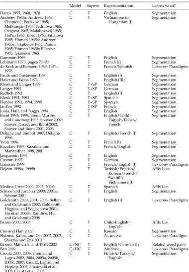
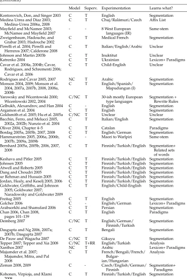
A chronological listing of earlier work (with very short characterizations) is given in Table 2. Several papers are co-indexed if they represent essentially the same line of work by essentially the same author(s).

Given the number of algorithms proposed, it is impossible to go through the tech-niques and ideas individually. However, we will attempt to cover the main trends and look at some key questions in more detail.

The problem has been approached in four fundamentally different ways, which we may summarize in the following way.

(a) Border and Frequency:In this family of methods, if a substring occurs with a variety of substrings immediately adjacent to it, this is interpreted as evidence for a segmentation border. In addition, frequent or somehow overrepresented substrings are given a direct interpretation as candidates for segmentation. A typical implementation is to subject the data to a compression formula of some kind, where frequent long substrings with clear borders offer the optimal compression gain. The outcome of such a compression scheme gives the segmentation. In addition, for those approaches which also target paradigms, stem–sufﬁx co-occurrence statistics are gathered given the segmentation produced, rather than all possible segmentations.

(b) Group and Abstract:In this family of methods, morphologically related words are ﬁrst grouped (clustered into sets, paired, shortlisted, etc.) according to some metric, which is typically string edit distance, but may include semantic features (Schone 2001), distributional similarity (Freitag 2005), or frequency signatures (Wicentowski 2002). The next step is to abstract some morphological pattern that recurs among the groups. Such emergent patterns provide enough clues for segmentation and can sometimes be formulated as rules or morphological paradigms.

(c) Features and Classes:In this family of methods, a word is seen as made up of a set of features—n-grams in Mayfield and McNamee (2003) and McNamee and Mayfield (2007), and initial/terminal/mid-substring in De Pauw and Wagacha (2007). Features which occur on many words have little selective power across the words, whereas features which occur seldom pinpoint a specific word or stem. To formalize this intuition, Mayfield and McNamee and McNamee and Mayfield use TF-IDF, and De Pauw and Wagacha use entropy. Classifying an unseen word reduces to using its features to select which word(s) it may be morphologically related to. This decides whether the unseen word is a morphological variant of some other word, and allows extracting the “variation” by which they are related, such as an affix.

(11)

[image:11.486.54.434.96.644.2]

Table 2

Very brief roadmap of earlier studies.

Model Superv. Experimentation Learns what?

Harris 1955, 1968, 1970 C T English Segmentation

Andreev 1965a, Andreev 1967, Chapter 2, Peršikov 1965; Melkumjan 1965; Fedulova 1965; Ožigova 1965; Malahovskij 1965; Hol’m 1965; Kordi 1965; Fitialova 1965; Fihman 1965a; Andreev 1965a; Jakubajtis 1965; Panina 1965; Fihman 1965b; Eliseeva 1965; Jakuševa 1965

C T Vietnamese to

Hungarian (I)

Segmentation

Gammon 1969 C T English Segmentation

Lehmann 1973, pages 71–93 C T French (I) Segmentation

de Kock and Bossaert 1969, 1974, 1978

C T French/Spanish Lexicon+ Paradigms

Faulk and Gustavson 1990 C T English (I) Segmentation

Hafer and Weiss 1974 C T English (IR) Segmentation

Klenk and Langer 1989 C T+SP German Segmentation

Langer 1991 C T+SP German Segmentation

Redlich 1993 C T English (I) Segmentation

Klenk 1992, 1991 C T+SP Spanish Segmentation

Flenner 1992, 1994, 1995 C T+SP Spanish Segmentation

Janßen 1992 C T+SP French Segmentation

Juola, Hall, and Boggs 1994 C T English Segmentation

Brent 1993, 1999; Brent, Murthy, and Lundberg 1995; Snover 2002; Snover, Jarosz, and Brent 2002; Snover and Brent 2001, 2003

C T

English/Child-English/Polish/ French

Segmentation

Deligne and Bimbot 1997; Deligne 1996

C T English/French (I) Segmentation

Yvon 1996 C T French (I) Segmentation

Kazakov 1997; Kazakov and Manandhar 1998, 2001

C T French/English Segmentation

Jacquemin 1997 C T English Segmentation

Cromm 1997 C T German Segmentation

Gaussier 1999 C T French/English (I) Lexicon+ Paradigms

Déjean 1998a, 1998b C T Turkish/English/

Korean/French/ Swahili/ Vietnamese (I)

Afﬁx Lists

Medina Urrea 2000, 2003, 2006b C T Spanish Afﬁx List

Schone and Jurafsky 2000, 2001a; Schone 2001

C T English Segmentation

Goldsmith 2000, 2001, 2006; Belkin and Goldsmith 2002; Goldsmith, Higgins, and Soglasnova 2001; Hu et al. 2005b; Xanthos, Hu, and Goldsmith 2006

C T English (I) Lexicon+ Paradigms

Baroni 2000, 2003 C T Child-English/

English

Afﬁx List

Cho and Han 2002 C T Korean Segmentation

Sharma, Kalita, and Das 2002, 2003; Sharma and Das 2002

C T Assamese Lexicon+ Paradigms

Baroni, Matiasek, and Trost 2002 C/NC T English/German (I) Related word pairs

Bati 2002 C/NC T Amharic Lexicon+ Paradigms

Creutz 2003, 2006; Creutz and Lagus 2002, 2004, 2005a, 2005b, 2005c, 2007; Creutz, Lagus, and Virpioja 2005; Hirsimäki et al. 2003; Creutz et al. 2005

C T Finnish/Turkish/

English

(12)

[image:12.486.50.429.91.656.2]

Table 2 (continued)

Kontorovich, Don, and Singer 2003 C T English Segmentation

Medina Urrea and Díaz 2003; Medina-Urrea 2006a, 2008

C T Chuj/Ralámuri/Czech Afﬁx List

Mayﬁeld and McNamee 2003; McNamee and Mayﬁeld 2007

- - 8 West European

languages (IR)

Same-stem

Zweigenbaum, Hadouche, and Grabar 2003; Hadouche 2002

C T Medical French Segmentation

Pirrelli et al. 2004; Pirrelli and Herreros 2007; Calderone 2008

C T Italian/English/Arabic Unclear

Johnson and Martin 2003b C T Inuktitut Unclear

Katrenko 2004 C T Ukrainian Lexicon+ Paradigms

´

Cavar et al. 2004a, 2004b; ´Cavar, Rodrigues, and Schrementi 2006;

´

Cavar et al. 2006

C T Child-English Unclear

Rodrigues and ´Cavar 2005, 2007 NC T Arabic Segmentation

Monson 2004, 2009; Monson et al. 2004, 2007a, 2007b, 2008, 2008a, 2008b

C T English/Spanish/

Mapudungun (I)

Segmentation

Yarowsky and Wicentowski 2000; Wicentowski 2002, 2004

C/NC T 30-ish mostly European type languages

Segmentation + Rewrite Rules

Gelbukh, Alexandrov, and Han 2004 C - English Segmentation

Argamon et al. 2004 C T English Segmentation

Goldsmith et al. 2005; Hu et al. 2005a C/NC T Unclear Unclear

Bacchin, Ferro, and Melucci 2005, 2002a, 2002b; Nunzio et al. 2004

C T Italian/English Segmentation

Oliver 2004, Chapter 4–5 C T Catalan Paradigms

Bordag 2005a, 2005b, 2007, 2008 C T English/German Segmentation

Hammarström 2005, 2006a, 2006b, 2007b, 2009a, 2009b

C - Maori to Warlpiri Same-stem

Bernhard 2005a, 2005b, 2006, 2007, 2008

C T Finnish/Turkish/English Segmentation+ Related sets of words

Keshava and Pitler 2005 C T Finnish/Turkish/English Segmentation

Johnsen 2005 C T Finnish/Turkish/English Segmentation

Atwell and Roberts 2005 C T Finnish/Turkish/English Segmentation

Dang and Choudri 2005 C T Finnish/Turkish/English Segmentation

ur Rehman and Hussain 2005 C T Finnish/Turkish/English Segmentation Jordan, Healy, and Keselj 2005, 2006 C T Finnish/Turkish/English Segmentation Goldwater, Grifﬁths, and Johnson

2005; Goldwater 2007;

Naradowsky and Goldwater 2009

C T English/Child-English Segmentation

Freitag 2005 C T English Segmentation

Golcher 2006 C - English/German Lexicon+ Paradigms

Arabsorkhi and Shamsfard 2006 C T Persian Segmentation

Chan 2006, Chan 2008, pages 101–139

C T English Paradigms

Demberg 2007 C/NC T English/German/

Finnish/Turkish

Segmentation

Dasgupta and Ng 2006, 2007a; 2007b; Dasgupta 2007

C T Bengali Segmentation

De Pauw and Wagacha 2007 C/NC T Gikuyu Segmentation

Tepper 2007; Tepper and Xia 2008 C/NC T+RR English/Turkish Analysis

Xanthos 2007 NC T Arabic Lexicon+ Paradigms

Majumder et al. 2007; Majumder, Mitra, and Pal 2008

C T French/Bengali/French/

Bulgar-ian/Hungarian

Analysis

Zeman 2008, 2009 C - Czech/English/German/

Finnish

Segmentation+ Paradigms Kohonen, Virpioja, and Klami

2008

(13)

Table 2 (continued)

Goodman 2008 C T Finnish/Turkish/English Segmentation

Golénia 2008 C T Turkish/Russian Segmentation

Pandey and Siddiqui 2008 C T Hindi Segmentation+

Paradigms

Johnson 2008 C T Sesotho Segmentation

Snyder and Barzilay 2008 C/NC T Hebrew/Arabic/Aramaic/ English

Segmentation

Spiegler et al. 2008 C T Zulu Segmentation

Moon, Erk, and Baldridge 2009 C T English/Uspanteko Segmentation

Poon, Cherry, and Toutanova 2009

C T Arabic/Hebrew Segmentation

Abbreviations: C = Concatenative; I = Impressionistic evaluation; IR = Evaluation only in terms of Information Retrieval Performance; NC = Non-concatenative; RR = Hand-written rewrite rules; SP = Some manually curated segmentation points; T = Thresholds and Parameters to be set by a human.

frequency techniques reminiscent of those of the (a) approaches can be applied. This strategy is targeted towards the special kind of non-concatenative morphology calledintercalated morphology11with the observation that, empirically, in those (relatively few) languages which have intercalated morphology, it does seem to depend on vowel/consonant considerations. In Xanthos (2007), the phonological categories are inferred in an unsupervised manner (cf. Goldsmith and Xanthos 2009) whereas in Bati (2002) and Rodrigues and ´Cavar (2005, 2007) they are seen as given by the writing system.

The ﬁrst two, (a) and (b), enjoy a fair amount of popularity in the reviewed collection of work, though (a) is much more common and was the only kind used up to about 1997. The last two, (c) and (d), have been utilized only by the sets of authors cited therein.

Let us now look at some salient questions in more detail. The following notation will be used in formal statements:

r

_w,_s,_b,_x,_y,_{. . .}_∈_Σ∗_{: lowercase-letter variables range over strings of some}

alphabetΣand are variously called words, segments, strings, and so forth.

r

_W,_S,_{. . .}_⊆_Σ∗_{: capital-letter variables range over sets of}

words/strings/segments.

r

_C_,_{. . .}_{: capital-letter caligraphic variables range over multisets of} words/strings/segments.

r

_{| · |}_{: is overloaded to denote both the length of a string and the cardinality} of a set.

r

_{w[i]: denotes the character at position}_i_{in the string}_{w. For example, if} w=hellothenw[1]=h.

r

_w[i_:_{j]: denotes the segment from position}_i_to_j_{(inclusive) of the string}_w. For example, ifw=hellothenw[1 :|w|]=hello.

(14)

r

_W_C_{is used to denote the set of words in a corpus}_C_.

r

_fp

W(x)=|{z|xz∈W}|: the (preﬁx) frequency ofx, that is, the number of

words inWwith initial segmentx.

r

_fs

W(x)=|{z|zx∈W}|: the (sufﬁx) frequency ofx, that is, the number of

words inWwith ﬁnal segmentx.

Subscript letters are dropped when understood from the context.

3.2 Border and Frequency Methods

3.2.1 Letter Successor Varieties. Most (if not all) authors trace the inspiration for their border heuristics back to Harris (1955). In fact, Harris deﬁnes a family of heuristics, all based on letter successor/predecessor varieties. They were originally presented as applying to utterances made up of phoneme sequences (Harris 1955), but they apply just the same to words, namely, grapheme sequences (Harris 1970). The basic counting strategy, labelled letter successor varieties (LSV) by Hafer and Weiss (1974), is as follows.

Given a set of wordsW, the letter successor variety of a stringxof lengthiis deﬁned as the number of distinct letters that occupy thei+1st position in words that begin withx inW:

LSV(x)=|{z[|x|+1]|z=xy∈W}|

Table 3 shows an example of a letter successor count on a tiny contrived wordlist. We may deﬁne the letter predecessor variety (LPV) analogously. For a given sufﬁx x, the LPV(x) is the number of distinct letters that occupy the position immediately precedingxin the words ofWthat end inx. LSV/LPV counts for an example word are shown in Table 4.

It should be noted that Harris (1955, page 192, footnote 4) explicitly targets the variety in letter successorstypes(i.e., is only interested in which letterseveroccur in the successor position, as opposed to being interested in their frequencies). For example, if there are two different letters occurring in successor position, one occurring a thousand times and the other once, Harris’s letter successor variety is still two—the same as if the two letters occurred once each. Subsequent authors have suggested that the full frequency distribution of thetokenletter successors carries a better signal of morpheme boundary. After all, if there is a significant token frequency skewing, this suggests that we are in the middle of coherent morpheme. Moreover, mere type counts may be influenced by phonotactic constraints (consonant after vowel, etc.), which come out less significant in token frequency counts (Goldsmith 2006, page 6). Already the earliest

Table 3

Example of LSV-counts for some example preﬁxes (bottom) based on a small example word list (top).

W={abide, able, abode, and, art, at, bat}

x a ab abe . . .

{z|z=xy∈W} {abide, able, abode, and, art, at} {abide, able, abode} ∅ . . .

(15)

Table 4

LSV counts ford-,di-,dis-, . . . ,disturbance-and LPV counts for-e,-ce,-nce, . . . ,-disturbance. All ﬁgures are computed on the Brown Corpus of English (Francis and Kucera 1964), using the 27 letter alphabet [a−z] plus the apostrophe. There are|W|=42,353 word types in lowercase.

LSV 13 20 21 6 1 1 3 1 1 1 1

d i s t u r b a n c e

LPV 0 1 1 1 1 1 1 19 6 12 25

follow-ups to Harris (Gammon 1969; Hafer and Weiss 1974; Juola, Hall, and Boggs 1994) experiment with replacing the raw LSV/LPV counts with the entropy of the character tokendistribution. The character token distribution after a given segment can be seen as a probability distribution whose events are the characters of the alphabet. The entropy of this probability distribution then measures how unpredictable the next character is after a given segment. In general, for a discrete random variableXwith possible values x1,. . .,xn, the expression for entropy takes the following form:

H(X)=− n

i=1

p(xi) log2p(xi)

Thus, with alphabetΣ, the letter successor entropy (LSE) for a preﬁxxis deﬁned as

LSE(x)=− c∈Σ

fp(xc) fp_(x) log2

fp(xc) fp_(x)

At least two authors (Golcher 2006; Hammarström 2009b) have questioned entropy as the appropriate measure for highlighting a morpheme boundary. Entropy measures how skewed the distribution is as a whole, that is, how deviant the most deviant member is, in addition to the second member, the third, and so on. If there is no mor-pheme boundary, the mormor-pheme continues with (at least) one character. Soonedeviant, highly predictable, character is necessary and sufficient to signal a non-break, and it is arguably irrelevant if there are second- and third-place, and so forth, highly predictable characters that also signal the absence of a morpheme boundary. For example, the character token distribution before-ngis shown in Table 5. Obviously, the fact that of the 3,352 occurrences of-ng, 3,258 of them are preceded by-i-, says that the absence of a morpheme boundary is highly likely. Now, does it matter that also another 35 are -o-versus only 4 for-e-? Entropy would also take into account the skewedness of-o-versus -e-, whereas for Hammarström (2009b) and Golcher (2006) only the skewedness of the most skewed character (i.e., the character that potentially constitutes the morpheme continuation) is interesting, in this example-i-. Therefore, these approaches only use the maximally skewed character to predict the presence/absence of a morpheme boundary. The letter successor max-drop (LSM) for a prefixxis defined as the fraction not occupied by its maximally skewed one-character continuation:

LSM(x)=1−maxc∈Σ

(16)

Table 5

The character token distributon for the character immediately preceding-ng, computed on the Brown Corpus of English (Francis and Kucera 1964).

-ng3,352

[image:16.486.52.434.219.272.2]

-n- 1 -l- l -h- l -e- 4 -u- 26 -a- 26 -o- 35 -i- 3,258

Table 6

Normalized LPV/LPE/LPM-scores for-e,-ce,-nce, . . . ,-disturbance. All ﬁgures are computed on the Brown Corpus of English (Francis and Kucera 1964), using the 27-letter alphabet [a−z] plus the apostrophe. There are|W|=42, 353 word types in lowercase.

d i s t u r b a n c e

LPV 0.03 0.03 0.03 0.03 0.03 0.03 0.70 0.22 0.44 0.92

LPE 0.0 0.0 0.0 0.0 0.0 0.0 0.74 0.28 0.38 0.81

LPM 0.0 0.0 0.0 0.0 0.0 0.0 0.83 0.53 0.37 0.85

Which one of LSV/LSE/LSM is the “correct” one? The answer, of course, depends on one’s theory of afﬁxation, for which the ﬁeld has no single answer (see Section 3.6, subsequently).

Empirically, however, the three measures are highly correlated. To compare the three, we normalize them to their maxima in order to get a “border” score≤1. The maximum achievable LSV is the alphabet size, so the normalized LSV(x) = LSV|Σ(|x). The maximum achievable LSE is a uniform distribution across the alphabet, so the normalized LSE(x) = −|Σ|·( 1_|LSE(x)

Σ|log2 1|Σ|). The maximum achievable LSM is a uniform

distribution across the alphabet, so the normalizedLSM(x)= 1LSM− (1x)

|Σ|. The predecessor

analogues LPV,LPE,LPM are obvious. Table 6 shows an example word and its normalized predecessor scores of the three kinds.

[image:16.486.53.430.619.664.2]

As in the example, the three different measures have nearly the same story to tell in general, at least for English. For the three measures, Table 7 shows the Pearson product-moment correlation coefﬁcient between the LPH/LPE/LPM-values of all ter-minal segments, as well as the Pearson product-moment correlation coefﬁcient between the LPH/LPE/LPM-ranks of all terminal segments. Most usages in the literature of the letter successor counts have been relative to other counts on the same language. In such cases, the rank correlations show that all three measures can be expected to have near identical effects.

Table 7

The Pearson product-moment correlation coefﬁcient between LPH/LPE/LPM-values (r) and the Pearson product-moment correlation coefﬁcient between LPH/LPE/LPM-ranks (r-rank). All values are computed on the Brown Corpus of English (Francis and Kucera 1964), using the 27-letter alphabet [a−z] plus the apostrophe. There are|W|=42, 353 word types in lowercase.

LPH&LPE LPE&LPM LPM&LPH

r 0.872 0.957 0.729

(17)

Harris (1955) and Hafer and Weiss (1974); for instance:

(a) Cutoff:By far the easiest way to segment a test word is ﬁrst to pick some cutoff thresholdkand then break the word wherever its successor (or predecessor or both) variety reaches or exceedsk.

(b) Peak and plateau:In the peak and plateau strategy, a cut in a wordwis made after a preﬁxxif and only ifLSV(w[1 :|x| −1])≤LSV(x)≥

LSV(w[1 :|x|+1]); that is, if the successor count forxforms a local “peak” or sits on a “plateau” of the LSV-sequence along the word.

(c) Complete word:A break is made after a word prefix (or before a word suffix) if that prefix (or suffix) is found to be a complete word in the corpus word listW.

These and similar strategies have been discussed and evaluated in various settings in the literature, and it is unlikely that any strategy based on LSV/LSE/LSM-counts alone will produce high-precision results. The example in Table 6 showing morpheme border heuristics on a speciﬁc word illustrates the matter at heart. Any intuitively plausible theory of afﬁxation should allow abundant combination of morphemes without respect to their phonological form, which predicts that high LSV/LSE/LSM values should emerge at morpheme boundaries. However, there appears to be no reason why the converse should hold—high LSV/LSE/LSM values could emerge in other places of the word as well. Indeed, any frequent character at the end or beginning of a word may also be expected to show high LSV/LSE/LSM around it, such as the-eat the end of disturbancewhich has higher values than, for example,-ance. Therefore, simply inferring that high LSV/LSE/LSM values indicate a morpheme border is not a sound principle in general.

A different (but less successful, even when supervised) way to use character se-quence counts is that associated with Ursula Klenk and various colleagues (Klenk and Langer 1989; Klenk 1991, 1992; Langer 1991; Flenner 1992, 1994, 1995; Janßen 1992). For each character bigramc1c2, they record, with some supervision in the form of manual curation, at what percentage there is a morpheme boundary before|c1c2, betweenc1|c2, after c1c2|, or none. A new word can then be segmented by sliding a bigram window and taking the split which satisﬁes the corresponding bigrams the best. For example, given a word singing, if the window happens to be positioned at -gi-in the middle, the bigram splits ng|,g|i, and |in are relevant to deciding whether sing|ing is a good segmentation. Exactly how to do the split by sliding the window and combining such bigram split statistics is subject to a fair amount of discussion. It became apparent, however, that the appropriateness of a bigram split is dependent on, for example, the position in a word—-edis likely at the end of a word, but hardly in any other position— and exception lists and cover-up rules had to be introduced, before the approach was abandoned altogether.

(18)

segment. Indeed, better candidates for morphemic segmentation are segments which are somehow overrepresented, that is, more frequent than random. There are various ways to deﬁne this property as well, including the following.

Overrepresentation as more-frequent-than-its-length: For a segment x of |x| charac-ters, it is overrepresented to the degree that it is more common than expected from a segment of its length. This applies to a segment in any position.

f(x)

|Σ||x|

Overrepresentation as more-frequent-than-its-parts: For a segmentx=c1c2. . .cnofn

characters, it is overrepresented to the degree that it is more common than ex-pected from a co-occurrence of its parts. This applies to a segment in any position.

f(c1c2. . .cn)

f(c1)f(c2). . .(cn)

Overrepresentation as more-frequent-as-suffix: For a segmentx, it is overrepresented to the degree that its probability as a suffix is higher than in any other (non-final) position. This applies to a segment in terminal position (but with obvious analogues for other positions).

With such measures, many authors have singled out afﬁxes above a certain over-representation-value threshold or overrepresentation-rank threshold.

Threshold values are unsatisfactory because typically there is no theory in which to interpret them. Although they may be set ad hoc with some success, such settings do not automatically generalize. Such considerations have led many authors to devise compression-inspired models for exploiting skewed frequencies. In particular, several different sets of authors have invoked Minimum Description Length (MDL) as the motivation for a given formula to compress input data into a morphologically analyzed representation.12

The MDL principle is a general-purpose method of statistical inference. It views the learning/inference process as data compression: For a given set of hypothesesHand data setD, we should try to ﬁnd the hypothesis inHthat compressesDmost (Grünwald 2007, pages 3–40). Concretely, such a calculation can take the the following form. IfL(H) is the length, in bits, of the description of the hypothesis; andL(D|H) is the length, in bits, of the description of the data when encoded with the help of the hypothesis, then MDL aims to minimizeL(H)+L(D|H).

In principle, all of the works that have invoked MDL in their ULM method act as follows. A particular wayQof describing morphological regularities is conceived that has two components which we may call patterns Pand data D. A coding scheme is devised to describe any P and to describe any collection of actual words with some speciﬁcPandD. A greedy search is done for a local minimum of the sumL(P)+L(D|P) to describe the set of words W(in some approaches) or the bag of word tokensC (in

(19)

(2006) particular wayQof describing morphological regularities is to allow for a list of stems, a list of affixes, a list of signatures (structures indicating which stems may appear with which affixes, i.e., a list of pointers to stems, and a list of pointers to suffixes). The search is then among different lists of stems, affixes, and signatures to see which is the shortest to account for the words of the corpus. Further details of such coding schemes need not concern us here, but for a range of options see, for example, Goldsmith (2001, 2006), Xanthos, Hu, and Goldsmith (2006), Creutz and Lagus (2007), Argamon et al. (2004), Arabsorkhi and Shamsfard (2006), Ćavar et al. (2004b), Baroni (2003), or Brent, Murthy, and Lundberg (1995).

It should be noted that the label MDL, in at least the terminology of Grünwald (2007, pages 37–38), is infelicitous for such cases where the P,D-search is not among different description languages, but among varations within a fixed language Q. For example, in the stem-affixes-signatures way of description (a specific Q), the search does not include other (possibly more parsimonious?) ways of description that do not use stems, affixes, or signatures at all. For the MDL-label to apply with its full philo-sophical underpinnings, the scope must include any possible compression algorithm, namely, any Turing machine. In this respect it is important to note that, compared to the schemes devised so far, Lempel-Ziv compression, another description language, should yield a superior compression (as, in fact, conceded by Baroni 2000, pages 146–147). MDL-inspired optimization schemes have achieved very competitive results in practice, however, and must be considered the leading paradigm to exploit skewed frequencies for morphological analysis.

3.2.3 Paradigm Induction.The next step after segmentation is to induce systematic alter-nation patterns, or (inflectional) paradigms,14and this is usually done as an extension of a border-and-frequency approach. For purposes of ULM, a paradigm is typically defined as a maximally large set of affixes whose members systematically occur on an open class of stems. For a number of reasons, finding paradigms is a major challenge. The number of theoretically possible paradigms is exponential in the number of affixes (as paradigms aresetsof affixes). Paradigms do not need to be disjoint; in real languages they are typically not. Rather, words in the same part of speech tend to share affixes across paradigms (Carstairs 1983). In addition, without any language-specific knowl-edge, basically the only evidence at hand is co-occurrence of stems and affixes (i.e., when a word occurs in the corpus it evidences the co-occurrence of a [hypothetical] stem and suffix making up that word). Paradigm induction would be an easy problem if all affixes thatcouldlegally appear on a worddidappear on each such word in a raw text corpus. This is, as is well known, far from the case. A typical corpus distribution is that a few lexemes appear very frequently but by far most lexemes appear once or only a few times (Baayen 2001). What this means for morphology is that most lexemes will appear with only one or a minority of their possible affixes, even in languages with relatively little morphology. Of course, there is also the risk that some rare affix, for example, the Classical Greek alternative medial 3p. pl. aorist imperative ending -σθων

13 As most approaches deﬁne their task as capturing the set of legal morphological forms, their goal should be to compressW, but see Goldwater (2007, pages 53–59) for arguments for compressingC.

(20)

(Blomqvist and Jastrup 1998), may not appear at all even in a very large Classical Greek corpus.

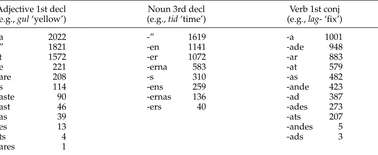
More formally, consider a morphological paradigm (set of sufﬁxes)Pthat is a true paradigm according to linguistic analysis. Ifklexemes that are inﬂected according toP occur in a corpus, each of theklexemes will occur in 1≤i≤ |P|forms. The number of formsithat a lexeme occurs in is likely not to be normally distributed. Most lexemes will occur in only one form, and only very few, if any, lexemes will occur in all |P| forms. It appears that for most languages and most paradigms, the number of lexemes that occur iniforms tends to decrease logarithmically ini(Chan 2008, pages 75–84). As an example, consider the three most common paradigms in Swedish and the frequency of forms in Table 8.

Works which have attempted nevertheless to tackle the matter of paradigms, at least for languages with one-slot morphology, include Zeman 2008, 2009, Hammarström (2009b), and Monson (2009). They explicitly or implicitly make use of the following two heuristics to narrow down the search space:

r

_{Languages tend to have a small number of paradigms (where “small”} means fewer than 100 paradigms with at least 100 member stems each).

r

_{Languages tend to have only small paradigms (where “small” means}

fewer than 50), that is, the number of afﬁxes in each paradigm is small. Agglutinative languages, which have several layers of afﬁxes, can be said to obey this generalization in the sense that each layer has few members, whereas conversely, the full paradigm achieves considerable size

combinatorially.

Although we know of no empirical evulation of them, in the impression of the present authors, the two heuristics appear to be cross-linguistically valid.

[image:20.486.54.432.508.663.2]

Chan (2006) is an exceptionally clean study of inducing paradigms, assuming that the segmentation is already given. The problem then takes the form of a matrix with

Table 8

The three most common paradigms in Swedish according to the SALDO lexicon and morphological resources (Borin, Forsberg, and Lönngren 2008), as computed on the SUC 1.0 corpus (Ejerhed and Källgren 1997) of 55,000 word types.

Adjective 1st decl Noun 3rd decl Verb 1st conj

(e.g.,gul‘yellow’) (e.g.,tid‘time’) (e.g.,lag- ‘ﬁx’)

-a 2022 -” 1619 -a 1001

-” 1821 -en 1141 -ade 948

-t 1572 -er 1072 -ar 883

-e 221 -erna 583 -at 579

-are 208 -s 310 -as 482

-s 114 -ens 259 -ande 423

-aste 90 -ernas 136 -ad 387

-ast 46 -ers 40 -ades 273

-as 39 -ats 207

-es 13 -andes 5

-ts 4 -ads 3

(21)

techniques from linear algebra, in particular Latent Dirichlet Allocation, to break the full matrix into smaller dense submatrices, which, when multiplied together, resemble the full matrix. There is only one humanly tuned threshold, namely, when to stop breaking into smaller parts.

3.3 Group and Abstract

In contrast to the methods that use a heuristic for finding morpheme boundaries, the grouping methods are much less sensitive to continuous segments. String edit distance is the most straightforward metric for which to find pairs or sets of morphologically related words (see, e.g., Gaussier 1999; Yarowsky and Wicentowski 2000; Schone and Jurafsky 2001a; Baroni, Matiasek, and Trost 2002; Hu et al. 2005a; Bernhard 2006, pages 101–117; Bernhard 2007; Majumder et al. 2007; Majumder, Mitra, and Pal 2008). In addition, as unsupervised methods for semantic clustering (e.g., Latent Semantic Analysis) and distributional clustering became more mature, these could be included as well (Schone and Jurafsky 2000, 2001a; Schone 2001; Baroni, Matiasek, and Trost 2002; Freitag 2005). More remarkable, however, is that Yarowsky and Wicentowski (2000) and Wicentowski (2002, 2004) have shown that frequency signatures can also be used to (heuristically) find morphologically related words. The example they use is sang versussing, whose relative frequency distribution in a corpus is 1,427/1,204 (or 1.19/1), whereassinged15 _versus_sing_{is 9/1,204 (Yarowsky and Wicentowski 2000, pages 209–} 210). This way, singcan be heuristically said to be parallel to sangrather thansinged, and indeed the distribution forsingedversussinge(its true relative) is 9/2, that is, much closer to 1.

Suppose now that groups of morphologically related words are somehow heuris-tically extracted. For example, one group might be {play, player, played,playing}and another might be {bark,barks,barked,barking}. The next step would be to find what is common among several groups, not just one. Abstracting morphological alternations given a family of groups is a thorny issue. For instance, Baroni, Matiasek, and Trost (2002) leave the matter largely in the exploration phase. Wicentowski (2004) presents a finished theory based on constraining the abstraction to find patterns in terms of prefix, suffix, and stem alternations.

The outstanding question for the group-and-abstract approaches, related not only to grouping but also to abstracting, is how to ﬁnd one and the same morphological process (umlauting, adding a sufﬁx, etc.) that operates over a maximal number of groups. The search space is huge, considering not only the group space but also the large number of potential morphological processes itself.

The group-and-abstract approaches are also characterized by the ubiquitous use of ad hoc thresholds. However, there are clear advantages in that they are in principle capable of handling non-concatenative morphology and in that issues of semantics (of stems) are addressed from the beginning.

The work by de Kock and Bossaert (1969, 1974, 1978), Yvon (1996), Medina Urrea (2003) and partly Moon, Erk, and Baldridge (2009) can favorably be seen as a mid-way between the border-and-frequency and group-and-abstract approaches as they rely on

(22)

Table 9

Example feature values for the wordsng˜ıthi˜ı(I went) andt ˜ug˜ıthi˜ı(we went) adapted from De Pauw and Wagacha (2007, page 1518).B=-features describe a subset at the start of the word form,E=-features indicate patterns at the end of the word, andI=-features describe patterns inside the word form.

class features

ng˜ıthi˜ı B=nB=ng B=ng˜ıB=ng˜ıtB=ng˜ıth B=ng˜ıthiI=g I=g˜ıI=g˜ıtI=g˜ıthI=g˜ıthi

E=g˜ıthi˜ıI=˜ıI=˜ıtI=˜ıthI=˜ıthiE=˜ıthi˜ıI=tI=thI=thiE=thi˜ıI=hI=hiE=hi˜ı

I=iE=i˜ı

t ˜ug˜ıthi˜ı B=tB=t ˜uB=t ˜ugB=t ˜ug˜ıB=t ˜ug˜ıtB=t ˜ug˜ıthB=t ˜ug˜ıthiI=˜uI=˜ugI=˜ug˜ıI=˜ug˜ıt

I=˜ug˜ıthI=˜ug˜ıthiE=˜ug˜ıthi˜ıI=gI=g˜ıI=g˜ıtI=g˜ıthI=g˜ıthiE=g˜ıthi˜ıI=˜ıI=˜ıt

I=˜ıthI=˜ıthiE=˜ıthi˜ıI=tI=thI=thiE=thi˜ıI=hI=hiE=hi˜ıI=iE=i˜ı

sets of four members with a particular afﬁxation arrangement (“squares”),16 _whose existence is governed much by the frequency of the afﬁxes in question.

3.4 Features and Classes

The features-and-classes methods share with the group-and-abstract methods the virtue of not being tied to segmental morpheme choices. As mentioned earlier, in this family of methods a word is seen as made up of a set of features which have no internal order— n-grams in Mayﬁeld and McNamee (2003) and McNamee and Mayﬁeld (2007), and beginning/terminal/internal segments in De Pauw and Wagacha (2007).

For example, Table 9 shows two words and their features in G˜ik ˜uy ˜u, a tonal Bantu language of Kenya. As designed by De Pauw and Wagacha (2007), initial (B=), middle (I=), or ﬁnal (E=) segments of a given word constitute its features. A majority of features enumerated this way will not be morphologically relevant, whereas a minority is. For example, in this case, I=h is just an arbitrary character without morpheme status, whereas I=ng˜ıthihappens to be equal to a stem. The idea is that arbitrary features such asI=h will be too common in the training data to provide a useful constraint, whereas a more specialized feature like I=ng˜ıthi might indeed trigger useful morphological generalization properties.

The input word listW thus transforms into a training set of word–feature pairs, which can be fed into a standard maximum entropy classifier. The next step is, for each word, to ask the classifier for thekclosest classes, namely, words (which will include the word itself andk−1 others with significant feature overlap). Clearly, such clusters may capture relations that string-edit-distance clustering does not. De Pauw and Wagacha

16 Based on the famousGreenberg square, which is a concrete means of illustrating the minimal requirement for postulating a paradigm: We need a minimum of two attested stems and two attested sufﬁxes (or in the general case arbitrary morphological processes), where both stems must occur with both sufﬁxes:

stemA+sx1 stemB+sx1 stemA+sx2 stemB+sx2

(23)

as preﬁxes, tonal changes, etc., may be abstracted from such clusters.

Clearly, feature-based methods provide an interesting new avenue for non-segmental and long-distance phenomena, but are so far largely unexplored and not free from thresholds and parameters.

3.5 Phonological Categories and Separation

These approaches specifically target the special kind of non-concatenative morphology called intercalated morphology (or templatic morphology or root-and-pattern mor-phology) famous mainly from Semitic languages, such as Arabic. They start out by assuming that graphemes can be subdivided into those that take part in the root, and those that take part in the pattern. For the languages so far targeted, Arabic (Rodrigues and Ćavar 2005, 2007; Xanthos 2007) and Amharic (Bati 2002), this is largely true, or a transcription is used where it is largely true. Rodrigues and Ćavar (2005, 2007) and Bati (2002) hard-code the transition from the graphemic representation of a word to its (potential) root and pattern parts. This can be said to constitute a strong language specific bias, tantamount to supervision. Xanthos (2007), on the other hand, starts out only by assuming that there existsa distinction between root and pattern graphemes and subsequently learns which graphemes are which. See Goldsmith and Xanthos (2009) for an excellent survey on how to do this (something which falls under learn-ing phonological categories rather than morphology learnlearn-ing). Basically, it is possible only because there are systematic combination constraints between different phonemes (approximated by graphemes); for example, vowels and consonants alternate in a very non-random manner.

Once each word is divided into its potential root and pattern, the morphology learning problem is similar to morphology learning given roots and sufﬁxes, that is, the typical model for learning concatenative morphology, where the task is to weed out noise, to decide where patterns (“sufﬁxes”) start and end, which patterns are spurious, and so on. All these authors who have addressed intercalated morphology use a variant of MDL (see the border-and-frequency techniques in Section 3.2). The accuracy of ULM on languages with intercalated morphology appears to be similar to the accuracy on other languages (cf. Section 4.3).

3.6 General Strengths and Weaknesses

(24)

yi occur in as many splits as possible. More precisely, the product, over all words,

of the number of splits for the parts x andy should be maximized. Formally, letxiyi

be the parts of wi induced by splitssi and letp(x)=|{i|x=xi}|=|{wi|xyi=wi}| be

the number of words in which x equals the ﬁrst part of the split and similarly let p(y)=|{i|y=yi}|=|{wi|xiy=wi}|be the number of words in whichyequals the last

part of the split. Then the task is to ﬁnd splits that maximize the following expression:

arg max [s1,...,s|W|]

wi∈W

p(xi)·p(yi)

For example, ifW={ad, ae, bd, be, cd, ce, ggg}, then the conﬁguration of splitsa|d, a|e, b|d, b|e, c|d, c|e, g|ggyields the product (2·3)6·(1·1).

Brent (1999) devises a precise, but more elaborate, way of constructingW fromB and S, but at the cost of a large search space, and whose global maximum is hard to characterize intuitively. The same holds for the extension by Snover (2002). Kontorovich, Don, and Singer (2003), Snyder and Barzilay (2008), Goldwater (2007), Johnson (2008), and Poon, Cherry, and Toutanova (2009) should also be noted for containing generative models.

Most approaches, of any of the kinds (a)–(d) described in Section 3.1, explicitly or implicitly target languages which have (close to) one-slot morphology, that is, a word (or stem) typically takes not more than one prefix and not more than one suffix. Many (indeed most; Dryer 2005) languages deviate more or less from this model. At first, it may seem that multi-slot morphology can be handled by the same algorithms as one-slot morphology, by iterating the process used for one-slot morphology. A decade of ULM has shown that the matter is not so simple, because heuristics for one slot languages do not necessarily generalize to the outermost slot of a multi-slot language.

The (c) and (d) approaches do not combine easily with the others but it is con-ceivable that the (a) and (b) type of approaches may be mutually enhancing. Results from the (a) methods may serve to cut down the search space for the (b) methods, and the (b) methods may provide a way to circumvent thresholds for the (a) methods. There is also the possibility of serial combination where, for example, the (a) methods target concatenative morphology and the (b)—or (c)—methods attempt the remaining cases. Presumably because most methods so far do not produce a clean, well-deﬁned result, various forms of hybridization of techniques by different authors have yet to be systematically explored.

Lastly, there are scattered attempts to address morphophonological changes in a principled way, though so far these have been developed in close connection with a particular segmentation method and target language (Schone 2001; Schone and Jurafsky 2001a; Wicentowski 2002, 2004; Tepper 2007; Kohonen, Virpioja, and Klami 2008; Tepper and Xia 2008).

4. Discussion

4.1 Language Dependence of ULM