Kumiko Tanaka-Ishii
∗Satoshi Tezuka
Hiroshi Terada
Graduate School of Information Science and Technology, University of Tokyo
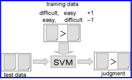
This article presents a novel approach for readability assessment through sorting. A comparator that judges the relative readability between two texts is generated through machine learning, and a given set of texts is sorted by this comparator. Our proposal is advantageous because it solves the problem of a lack of training data, because the construction of the comparator only requires training data annotated with two reading levels. The proposed method is compared with regres-sion methods and a state-of-the art classification method. Moreover, we present our application, called Terrace, which retrieves texts with readability similar to that of a given input text.
1. Introduction
Readability assessment is an important NLP issue with much application in the domain of language education. The capability to automatically judge the readability of a text would greatly help language teachers and learners, who currently spend a great deal of time skimming through texts looking for a text at an appropriate reading level.
Substantial previous work has been done over the past decades (Klare 1963, DuBay 2004a, 2004b). Early work generated measures based on simple text statistics by as-suming that these reflect the text reading level. For example, Kincaid, Fishburne, and Rodgers (1975) assumed that the lengths of words and sentences represent their re-spective difficulty. Chall and Dale (1995) used a manually constructed list of words assumed to capture the difficulty of vocabulary. These measures are easy to use but difficult to apply to languages other than English, because some features, such as word length, are specific to alphabetic writing. Such methods, however, do not compete with recent methods based on more sophisticated handling of language statistics. Collins-Thompson and Callan (2004) proposed a classification model by constructing different language models for different school grades (Si and Callan 2001), and Schwarm and Ostendorf (2005) applied a support vector machine (SVM). Both of these methods outperform classical methods and are less language-dependent.
These new methods, however, have a serious problem when implementation is at-tempted for multiple languages: the lack of training corpora. Large amounts of training data annotated with 12 school grades have not been at all easy to obtain on a reasonable scale. Another possibility might have been to manually construct such training data,
∗University of Tokyo Cross Field, 13F Akihabara Daibiru, 1-18-13 Kanda Chiyoda-ku, Tokyo, Japan. E-mail: [email protected].
but humans are generally unable to precisely judge the level of a given text among 12 arbitrary levels. The corpora therefore have to be constructed from academic texts used in schools. The amount of such data, however, is limited, and its use is usually strictly limited by copyrights. Thus, it is crucial to devise a new method or approach that allows readability assessment by using only generally available corpora, such as newspapers.
Given a single text, it is hard to attribute an absolute readability level from among 12 levels, but given two texts, there should be a better chance of judging which of them is more difficult. This intuition led to the new model presented in this article. Our idea is based onsorting, which is implemented in two stages:
r
A comparator is generated by an SVM. This comparator judges the relative readability of two given texts.r
Given a set of texts, the texts are sorted by the comparator with a sorting algorithm. In our case, we used a robust binary insertion sort, as explained in further detail later in this article.The first step requires a training corpus, but because the comparator only judges which of two texts is more difficult, the texts of a corpus need only be labeled according to two different levels. Two sets of texts—one difficult, the other easy—are far easier to obtain than a training corpus annotated for 12 different levels. Overall, our model of readability thus differs from previous regression or classification models.
Applying this new method, we also present an application, calledTerrace, which is a system that retrieves a text with readability similar to that of a given input text. Terrace was originally motivated by a faculty request made by teachers of multiple foreign languages. The system currently works for English and Japanese, and the languages will be extended to include Chinese and French.
Note that we donotclaim that our model and method is better than existing meth-ods. Although our method does compete well with previous methods, the classification approach used in any given scenario should remain the most natural, relevant method. The intention of this article is simply to propose an alternative way of handling read-ability assessment, especially when adequate training corpora annotated with multiple levels are not available.
2. Related Work
Readability, in general, describes the ease with which a text document can be read and understood. Readability is studied in at least two different domains, those of coherence (Barzilay and Lapata 2008) and language learning. Readability in this article signifies the latter, for both a mother tongue and a second language.
Even within this domain, substantial previous work has been done (Klare 1963; DuBay 2004a, 2004b). DuBay (2004a) writes that:
By the 1980s, there were 200 formulas and over a thousand studies published on the readability formulas attesting to their strong theoretical and statistical validity (p. 2).
Regarding the first type, many researchers have reported how various features affect the readability of text in terms of vocabulary, syntax, and discourse relations. Recently, Pitler and Nenkova (2008) presented an impressive verification of the effects of each kind of feature and found that vocabulary and discourse relations are prominent, although other features are not negligible.
The focus of the current work, however, is not on what feature set to consider, so we use the same features throughout the article, as explained further in Section 3.1. Rather, the focus of this article is onmappingthe extracted feature values to a readability norm. So far, two models have been used for this: regression and classification.
In regression, readability is given by a score based on a linearly weighted sum of feature values. Early methods, from the Wannetka formula (Washburne and Vogel 1928), to the recent methods of Flesch–Kincaid (Kincaid, Fishburne, and Rodgers 1975) and Dale–Chall (Chall and Dale 1995), are of this kind. Elaboration of such regression methods in a more modern context could proceed through a generalized linear model based on estimation of the weights by machine learning, although we have not found such an approach within the literature of readability assessment for language learning. Our proposal is compared with such an enhanced version of regression in Section 8.
In classification, readability is segmented by academic grades, and the assessment is conducted as a classification task. The first is implemented by means of statistical classification modeling, as reported in Collins-Thompson and Callan (2004) and Si and Callan (2001). The authors used a language model (unigrams) and a naive Bayes classifier by presuming different language models for each reading level. A language model Mi is constructed for each level of readability iby using different corpora for
each level. The readability of a given text T is assessed using the formulaL(Mi|T)=
Σw∈TC(w) log Pr(w|Mi), wherewdenotes a word in textT,C(w) denotes the frequency
ofw, and Pr(w|Mi) denotes the probability ofwunderMi. The second is based on an
SVM (Schwarm and Ostendorf 2005) and the authors also studied the effect of statistical features, such asn-grams and syntactic features.
In these papers, the readability norms are represented by means of scores and classes of readability. That is, given a single text, the system assigns a value correspond-ing to a school grade. The result is easy to understand, and various applications have been constructed with this type of scoring. This solution only works, however, when a sufficient amount of training data with annotations regarding multiple levels is pro-vided. Usually, the availability of training data in readability assessment is limited, even for school grading. This is due to the inherent difficulty of classifying the readability of a text into 12 grades, making it difficult to uniformly construct a large set of training data. Moreover, the copyright issue is more serious for academic texts.1Given this situation, when readability assessment is modeled by regression or classification, a research team wanting to apply these previous methods faces the problem of assembling training data, as we did for over a year.
In this article, the readability norm is designed in a completely different way: Given two texts, a comparator judges which is more difficult. By applying this comparator, a set of texts is sorted. The readability of a text is assessed by searching for its position
within the sorted texts. The norm is thus considered as the location of a text among an orderedset of texts. Our approach linguistically enhances assessment of the readability of a text as therelativeease compared to other texts, not as the absolute difficulty of the text. The root of this idea has been presented in two articles of which we are aware. In Inui and Yamamoto (2001), the readability ofsentencesfor deaf people is judged by a comparator generated by an SVM. In addition, Pitler and Nenkova (2008) presented a comparison of texts in terms of difficulty by using an SVM. Similarly to what we present in Section 3.1, those authors propose constructing a comparator by using an SVM to compare two sentences or texts with multiple features. However, neither further applied this approach to obtain readability assessment based on sorting. Our contribution in this study is therefore that we show how a machine learning method can be used as a comparator and applied tosorttexts.
Our method can be situated more generally among machine learning methods for ranking, where the methods learn so that they rank a set of elements given a set of ordered training data. Various methods have been proposed so far. In one of the earliest attempts, Cohen, Schapire, and Singer (1998) obtain a function that scores the probabil-ity that an element is ranked higher than another, and rank all elements by maximizing the sum of the pairwise probabilities. In another, Joachims (2002) applies an SVM to rank elements, by devising the input vector by subtraction of feature values. In more recent studies, such as Xia et al. (2008), an attempt is made to directly obtain the ranking function for the whole ordered training data, not as a composition of pairwise function application between elements. Among these methods, our proposal is unique in two ways. First, none of the previous methods, as far as we know, proposed discretized ranking based on sorting. Second and most importantly, all previous methods assume the existence of fully ordered training data. In contrast, as emphasized by our problem described in this section, such training data are difficult to acquire in the readability domain, and we have to devise a method which works even when very limited training data are all that is available. Our contribution lies in our study of the possibility of using a learning-to-rank method even when learning data are only partially available. Such an approach can be further considered for learning-to-rank methods in general in future work.
3. The Method
In our method, a comparator of the level of difficulty of two texts is generated by using machine learning and then the comparator is applied to sort a set of texts. The method has two parts:
r
construction of the readability relation<, andr
sorting and searching texts by using the relation.These tasks are explained in the following sections.
3.1 Readability Comparator
The readability comparator is constructed by applying machine learning. Given texts a,b∈S, whereSis a set of texts, feature vectorsVaandVbare constructed. By applying
an operator◦,Vabis constructed asVa◦Vb. WhenVabis entered into the comparator, the
Figure 1
Construction of a comparator using an SVM.
the output is binary, we use an SVM to construct the comparator (see Figure 1). Note thatVabandVbaare not the same. Reversibility of a feature vector is thus not obvious in
our work, but ideally, when the judgment forVabis 1, that forVbawill be –1.
In terms of constructing a feature vector Va for a texta, substantial features have
been proposed (Klare 1963; DuBay 2004a, 2004b; Schwarm and Ostendorf 2005; Pitler and Nenkova 2008). In this work, we only utilize the most basic features of vocabulary in terms of word frequencies for three reasons. First, as stated in Section 2, because the focus of this article is not to study the set of features, it is best to set the feature issue aside and use only the most fundamental features. Even then, there are many viewpoints to be verified, as will be seen in Sections 7–9. Furthermore, we have to take into account the pros and cons of various features, because naive features only capture coarse, default trends and could degrade performance. For example, the text length in our data tends to be longer for more difficult texts, thus having a bad influence on short, higher-grade texts and long, lower-grade texts. Therefore, in this article, we only consider simple features regarding vocabulary. Second, previous work has argued for the fundamental nature of vocabulary as a factor in readability (Alderson 1984; Laufer 1991; Pitler and Nenkova 2008). Third, some features other than word frequencies are language-dependent in terms of the writing system, corpus availability, and perfor-mance of NLP analysis systems. For example, average word length, used in the Flesch– Kincaid approach, cannot be applied to Japanese. Thus, we have focused on features that are available for any language, so that the performance becomes comparable across languages.
The features we use are as follows. There are two factors within vocabulary: the local and global factors. The local factor is what words are used and how frequently they ap-pear within a text, whereas the global factor indicates the degree of readability of these words among the overall vocabulary. Both are considered within this article, as follows:
Local: the frequency of each word divided by the frequency of the number of words in the text (this is calledrelative frequencyhere).
Global: the log frequency of words obtained from a large corpus.
Local frequency is the most basic statistic used in machine learning methods. Relative frequency is used to avoid the influence of text length, as mentioned above.
attributed to all words should affect the difficulty levels of texts. In Chall and Dale (1995), the authors counted the number of words not appearing in a list of the most basic 3,000 words, in order to judge vocabulary difficulty, but the plausibility of such a list is difficult to evaluate and such lists might not exist for languages other than English. An alternative is to use word lists with familiarity scores, such as the MRC list in English (Database 2006) or the Amano list in Japanese (Amano and Kondo 2000), but such lists are costly to generate and the word coverage is limited. Instead, we decided to use the log frequency obtained from several terabytes of corpora, because the psychological familiarity score is known to correlate strongly with the log frequency obtained from corpora, as reported in Tanaka-Ishii and Terada (2009) and Amano and Kondo (1995). Tanaka-Ishii and Terada show that log frequency correlates better for larger corpora. Thus, as will be explained in Section 6, Web corpora consisting of 6 terabytes for English and 2 terabytes for Japanese—possibly the largest corpora available for the two languages—were used to obtain the log frequencies.
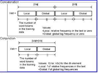
Local and global features are extracted for all words of the two texts aand b to be compared. The final vector is generated by applying an operator◦, such thatVab=
Va◦Vb. Two simple possibilities for the operation◦are the following:
Concatenation: concatenateVb’s elements after the elements ofVa.
Conjunction: produce a new value for theith element ofVabfrom theith elements ofVa
andVbby some function. Typical possibilities for such a function are subtraction
and division.
The two possible vectors forVabare explained by the illustration in Figure 2. The upper
[image:6.486.49.390.382.641.2]half of the figure shows Vab generated by concatenation. Because the comparator is
Figure 2
constructed by machine learning, the dimension of the vectors is four times the number of word tokens that appear in the training data. Each kind of word has a location in a vector, which appears four times withinVab: twice in eachVa and Vb for local and
global features. The first half denotesVa, and the second half denotesVb. In the first half
ofVa, the vector values are the relative frequencies for words appearing in texta, or zero
otherwise. For the second half ofVa, the values are log frequencies measured in a large
corpus for the words appearing ina, or zero otherwise.Vb is constructed in a similar
manner, and the two vectors are concatenated.
In contrast, in the case of conjunction, the dimension of the vector remains twice the number of word tokens appearing in the training data, as illustrated in the lower half of Figure 2. Theith dimension ofVabis calculated as a function of theith values of
Va andVb. Pitler and Nenkova (2008) are likely to have used subtraction within their
experiment.2For this reason, among various other possible functions for the conjunction of two vector values, we also used subtraction.
Construction of a comparator requires training data. Because the comparator judges the difficulty between two texts, the training data contains two sets of texts, a setLdof
a relatively difficult level and a set Le of a relatively easy level. The SVM is trained
on a combination of texts taken fromLe andLd. The training data can combine up to
2× |Le| × |Ld|. For example, if|Le|=|Ld| = 600, the number of data points for training
could amount to 720,000. Whether learning can fully exploit such combined training data is an interesting issue, which is examined in Section 8.
After training, for two given texts a and b, the relative difficulty is judged by inputtingVabinto the SVM. In this phase, if a new word which was not in the training
corpora appears in eitheraorb, the word is ignored for the purposes of this work.
3.2 Sorting and Searching Texts
With a comparator thus constructed, the texts of S are sorted. Further, readability assessment is performed by searching for the position of a text within the sorted texts.
The sorting and searching algorithms can be chosen from among the basic ones already established within computer science. There are further requirements, however, as follows:
r
Searching must be as fast as possible for the actual application.r
Sorting and searching should be implemented with the same procedure, given the nature of the application, as will be explained in Section 5. Moreover, sorting should be done incrementally to facilitate the addition of texts.r
Sorting must be made robust to overcome judgment errors made by the comparator.Given the first two requirements, we chose binary insertion sort and binary sorting from among various sorting and searching algorithms, because it provides one of the fastest search methods.
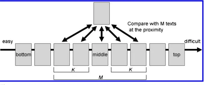
To meet the last requirement, the algorithm is made robust by performing multiple comparisons at one time, as explained here. In binary insertion sort, given a new text, the insertion position is searched for among the previously sorted texts (from the easiest text to the most difficult text), and the text is inserted between two successive textsi andi+1, where the text is more difficult than theith easiest text and it is easier than thei+1th text. Through repetition of this operation, all texts are sorted. Because our comparator is generated using an SVM, one sole comparison could lead to an erroneous result. Moreover, one comparison error could lead to disastrous sorting results with a binary sort, because binary search changes the insertion position significantly, especially at the beginning of the search procedure.
To avoid such comparison mistakes, the comparison judgment is made through multiple comparisons with texts located at the proximity of each position. The number of multiple comparisons is called the width and is denoted as M=2K+1, with K being a positive natural number, as illustrated in Figure 3. Mis dynamically changed during the search procedure by narrowing it down to indicate the exact position. The procedure starts with a given set of textsSand an empty setSS. At each judgment, a text to be inserted is removed fromSand inserted intoSS. The procedure proceeds as follows:
1. Obtain a textxfromS. IfSSis empty, the textxis put intoSSand another textxis obtained fromS.
2. The texts ofSSare already sorted and are indexed byi=1. . .n, where i=1 is the easiest andi=nis the most difficult. Searching is done using three variables, which are initialized as follows:bottom←1;top←n; middle← (top+bottom)/2. The widthMis set as follows:M=2×K+1 (K∈N).
3. IfM>(top−bottom)/2, thenK← (top−bottom)/2. A change inKalso changes the value ofM, which is always set to 2×K+1.
4. Comparexwith texts ati=middle−K...middle+K. If more than K texts are judged as difficult, thentop←middle−1. Otherwise,bottom← middle+1.
[image:8.486.49.390.499.641.2]5. Iftop<bottom, then insertxbefore thebottom. Otherwise, go to step 3.
Figure 3
6. Insertxbeforebottom.
7. If|S|>1, then go to step 1. Otherwise, the procedure is complete.
The complexity for sorting a set|S|amounts toO(C|S|2), whereCis the maximum value of M. Because the time complexity required for insertion is log n, it might seem that the total time complexity is O(C|S|log|S|), but this is not the case: Random access for binary insertion requires the whole data structure to be implemented by an array, which requires copying of the wholeSSat every insertion. Note that the sorting speed at this point does not affect the usability of our application, since the text collection is sorted offline (as explained in Section 5).
On the other hand, the searching speed does affect the usability. For sorted texts, the readability of a text is assessed by searching for its insertion position. The searching is done by binary search, through the same procedure in steps 2 to 6. The computational complexity isO(Clog|SS|), where C is the maximum value ofM.
4. Pros and Cons of the Proposed Method
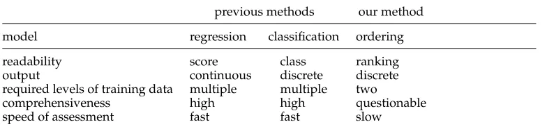
[image:9.486.52.444.570.663.2]Now that we have explained our method, we compare it with the previous models of regression and classification mentioned in Section 2. The comparison is summarized in Table 1.
In previous work that we mentioned, the readability of a text is represented by a score or class, which typically has been indicated in terms of school grades (third row). In contrast, readability in our method is presented as a position among texts, indicating the ranking of a text situated globally among the other texts of SS. Considering the nature of the output of assessment, the regression method is continuous, in that feature values are mapped to scores within a continuous range, whereas classification and our method are both discrete, in that the former gives a class and the latter gives a rank (fourth row).
This fundamental difference gives rise to pros and cons. Above all, the advantage of our method is that it facilitates the construction of training data (fifth row), because it requires only two sets of typically difficult and easy texts. Here, what kinds of corpora the regression method requires in the modern machine learning context has not been clarified because of the lack of previous work in machine learning regression. However, our empirical results, shown in Section 8, suggest that the two sets of difficult and easy training data will not be sufficient, and machine learning regression requires texts labeled with scores for different levels.
Table 1
Qualitative comparison of our method with previous methods.
previous methods our method
model regression classification ordering
readability score class ranking
output continuous discrete discrete
required levels of training data multiple multiple two
comprehensiveness high high questionable
At the same time, there are disadvantages to our model. First, because the method only outputs a relative ranking, applications must be re-designed differently from those in the previous work (sixth row). It could be said that whena>bfor documentsaand b, thenacontains more unfamiliar words as tokens. Even if two texts are next to each other, however, their readability could be very different. For example, texts of grades 1 and 11 could be next to each other in a collection if it lacks texts from grade 2 to 10. An application system generated using our model must cope with this new problem caused by this lack ofabsolutenessfor the readability norm. In the next section, we show how this problem is dealt with in Terrace through the use of graphical representation.
Second, the scores and classes of regression and classification are used to hash the position of texts within the readability norm. On the other hand, because our method lacks scores, the location of a text must always be searched for. Thus, the previous methods require onlyO(1) time for searching, whereas our method requires a certain amount of time before a response is obtained. Therefore, it must be verified that an ap-plication works within a reasonable response time when handling a large text collection. In Section 9, we show that the response time is indeed within a reasonable time.
5. Terrace: An Application
As mentioned in Section 1, creation of this system was motivated by a request from faculty members who teach multiple foreign languages. These teachers must look for up-to-date reading materials with appropriate reading levels every day. This requires scanning through newspapers and Web resources. The teachers’ request was that we construct a system that would facilitate this text search task. More precisely, given a sample text used within the classroom, the system should return texts of similar levels of readability from among newspaper articles and other on-line archives.
At the beginning of this project, we tried to apply Schwarm and Ostendorf (2005) and Collins-Thompson and Callan (2004). Because the request covered multiple lan-guages, though, we faced the corpus construction problem in different languages. This problem was serious, to the extent that training corpora used in published work in English were unavailable. We were forced to look for another path towards building the requested system without annotated corpora having academic grades.
The problem of returning texts of similar readability does not necessarily require intermediating a score/class, because both the input and output are texts. Thus, chang-ing our way of thinkchang-ing, we looked for another readability norm, which led to the framework presented so far.
Terrace is a Web-based system in which the user uploads a text, and the system returns texts of similar readability from among a collection of texts usable as teaching materials, which are crawled for and obtained from the Web. Currently, Terrace works for English and Japanese. The number of languages is currently being increased.
Figure 4 shows an example of giving an input text to Terrace. After the user uploads the text and clicks the Terrace search button, a page like that shown in Figure 5 is displayed.
Figure 4
Screen shot of Terrace input.
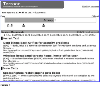
Figure 5
Screen shot of Terrace result for the given input.
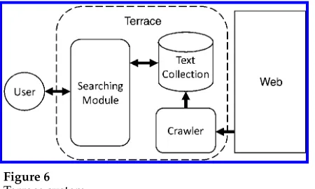
[image:11.486.52.393.287.581.2]Figure 6 Terrace system.
The texts with the closest readability are shown below, and then easier texts are listed. Further down, more difficult texts are listed. By clicking on any of these texts, the user can obtain texts with the desired readability.
This functionality of Terrace is implemented via two modules, one each for search-ing and for crawlsearch-ing, as shown in Figure 6. The crawler collects texts from news sites and other related archive sites every day, and the module incrementally sorts the collected documents. These texts are searched upon a user request.
6. Data for Evaluation
In the rest of this article, the proposed method and the Terrace system are evaluated. The key question to be considered through the evaluation is whether the comparator can discern slight differences in the readability levels of test data from only two sets of training data that are roughly different.
The proposed method was tested for English and Japanese. The data is summarized in Table 2, where the upper block corresponds to English and the lower to Japanese. For
Table 2
Training and test data.
English Data
label corpus levels # of Texts # of Words
Training & TD1-E Time normal 600 623,203
children 600 259,163
TD2-M-E AtoZ 27 levels (5 grades) 674 1,060,557
TD2-F-E English textbook 5 levels (linear) 153 114,054
Japanese Data
label corpus levels # of Texts # of Words
Training & TD1-J Asahinewspaper normal 600 841,289
children 600 533,568
both languages, there were training data and test data. The test data consisted of two sorts:
TD1: A collection of texts taken from the same kind of data as the training data. TD2: A collection of texts unrelated to the training data and originally assigned levels
or a linear ordering. These levels and ordering were used as the correct ordering in our work.
TD2 further consisted of two kinds of data in each language: data for learners of their mother tongue (i.e., children and students) and data for learners of a foreign language. These are labeled as TD2-M and TD2-F, respectively.
For English, the training data were taken fromTime(Time 2008) andTime For Kids (TimeForKids 2008). We downloaded 600 articles (that is,|Ld|=|Le|=600), of which 100
were used as TD1-E. The total number of different words in TD1-E is 22,736, which is the dimension of the feature vector of a text when TD2 is used as the text data.3When using subtraction as◦, the dimension is doubled (for local and global), and when using concatenation, the dimension is four times this value. TD2-M-E consisted of the data set called AtoZ, which can be purchased (ReadingA-Z.com 2008). Each of the texts in this data set is labeled by 27 levels and graded by 5 levels. TD2-F-E consisted of the English textbooks used in Japanese junior high and high schools (Morizumi 2007; Yoneyama 2007). These texts are classified into five grades and also linearly ordered; that is, the texts become more difficult in their order of appearance in the textbooks. These levels and orders originally attached to the data were used as the gold standard in this study. For the global frequency, we used the log frequency of each word as measured from almost 6 terabytes of Web data in English, scanned in the autumn of 2006 (Tanaka-Ishii and Terada 2009).
For Japanese, the training data and TD1-J were taken from Asahi newspapers (AsahiNewspaper 2008; KodomoAsahi 2008). Six hundred (600) articles were acquired, and 100 of these were used as TD1-J. The total number of different words in this training data is 48,762.4 TD2-M-J consisted of Japanese junior high and high school textbooks with six grades, which also appeared in a linear order (Miyaji 2008). TD2-F-J consisted of the texts used in the Japanese language proficiency test (JEES 2008). The texts in this data set are classified into four levels and not linearly ordered. For the global frequency, we used the log frequency of each word as measured from almost 2 terabytes of Web data in Japanese, scanned in the autumn of 2006.
The other evaluation settings were as follows. As the SVM (Joachims 1998, 1999), we used LIBSVM (Chang and Lin 2001). The SVM training was done using the parameters of cost = 0.1 and gamma = 0.00001 with a Gaussian kernel. The value ofKused in robust sorting (Section 3.2) wasK=2.
7. Evaluation of the Comparator
The basic performance was first tested using TD1. Because |Ld| =|Le| = 600, 500 texts
were chosen and paired randomly, and 2×500 = 1,000 pairs were used for training. The factor of 2 is necessary, because a pair can be used twice by exchanging the comparison orderVedandVde. The remaining 100 texts were randomly paired and tested. The results
3 Words are transformed into their standard forms using the Lancaster algorithm (Paice and Husk 2008). Moreover, we do not use feature selection, because it has been reported that the distribution of function words also counts with respect to readability (Collins-Thompson and Callan 2004).
Table 3
Accuracy of the comparator for different operators and features tested on TD1.
English
Concatenation 91.67% Subtraction 94.27%
Japanese
Concatenation 95.47% Subtraction 95.47%
presented here were produced through six-fold cross-validation, and each fold was further repeated five times by changing the pairing of training and testing (i.e., total execution was done 30 times to obtain one performance value).
Table 3 shows the accuracy for English (upper block) and Japanese (lower block). The rows of a block represent the different operators explained in Section 3.1. Overall, the scores were above 90%.
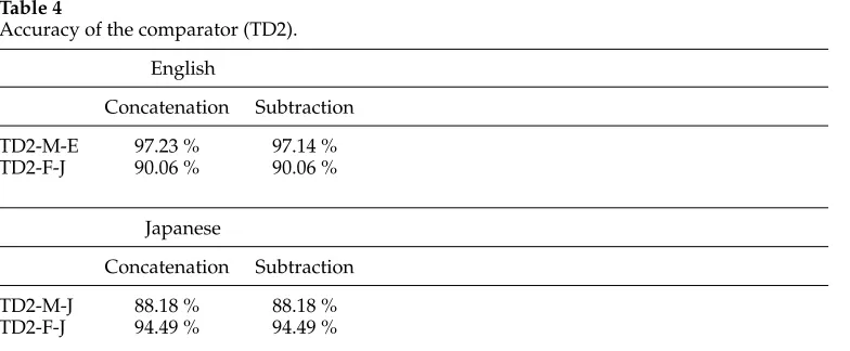
The comparator performance for TD2 was also investigated (Table 4). Here, the training data amount was set to 2×600. The accuracy was measured for all pairs of texts with different levels. For TD2-M-E, all five levels were considered, whereas for the linearly ordered TD2-F-E and TD2-M-J, the levels were considered by grade (that is, five levels for TD2-F-E and six levels for TD2-M-J). The accuracy reported here is the average of execution done five times by changing the random pairing for the training data. The performance was, in general, lower than that for TD1, but still stayed close to 90%. For the operator ◦, whether concatenation or subtraction was used made no difference. Therefore, from here on, the operator◦is set to concatenation.
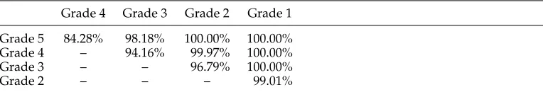
[image:14.486.50.442.503.665.2]To evaluate the classification performance in more detail, the accuracy for every two-class combination was determined for TD2-M-E in English, as shown in Table 5. Because TD2-M-E has five grades, the columns indicate the 1st to 4th grades, whereas the rows indicate the 2nd to 5th grades. The evaluation thus forms a 4×4 table, where each cell indicates the accuracy of distinguishing the two–class pairs for the row and column.
Table 4
Accuracy of the comparator (TD2).
English
Concatenation Subtraction
TD2-M-E 97.23 % 97.14 % TD2-F-J 90.06 % 90.06 %
Japanese
Concatenation Subtraction
Table 5
Classification results between two classes, tested for TD2-M-E in English.
Grade 4 Grade 3 Grade 2 Grade 1
Grade 5 84.28% 98.18% 100.00% 100.00% Grade 4 – 94.16% 99.97% 100.00%
Grade 3 – – 96.79% 100.00%
Grade 2 – – – 99.01%
The closer to the diagonal, the more difficult the classification task was, because the levels to be distinguished became closer to each other. The results reflect this ten-dency, with lower values for cells closer to the diagonal. In particular, the performance for discerning grades between pairs of the 4th and 5th grades was poor. Distinction between the 1st/2nd and 2nd/3rd grades was more successful than that between the 3rd/4th and 4th/5th grades, since the lower the grades the easier it is to discern two given successive school levels.
Before going on to actually sort text using the comparator, we verified how abnor-mal our generated comparator was. Ideally, we want a complete ordering of the set, and for this the comparator must obey certain laws in the sense of mathematical sets. A comparator is considered abnormal if it does not obey two laws:
Reversibility: Texts a,b are defined as reversible if b<a and a>b both hold. This corresponds to the law that whenVab’s value is +1, thenVba’s value must be –1
and vice versa.
Transitivity: Ifa<bandb<c, thena<c.
Especially for transitivity, in an ordered set this law is the primary requirement that must be fulfilled among ordered elements. If transitivity does not hold in many triples, we have to introduce partial ordering instead of the total ordering considered thus far.
The anomalies were measured by using the four TD2 data sets. For all pairs and triples of TD2, we tested the reversibility and transitivity for all possible pairs and triples by changing the random pairing of test data (TD1) five times. For reversibility,
r
10 pairs out of 226,801 for TD2-M-E were non-reversible once,r
1 pair out of 11,628 for TD2-F-E was non-reversible once, andr
all pairs for all other data and random pairings of training data werereversible.
Such strong results were obtained because the training was done by reversing the order of the pairs (thus, the SVM learned bothVed as +1 andVdeas –1.) Similarly, for
transitivity,
r
one triple out of 50,803,424 of TD2-M-E was non-transitive once, andr
all triples for all other data and random pairings of training data weretransitive.
8. Evaluation of Sorting
Since the basic results have been clarified thus far, we will now report the results for concatenation for a more global evaluation of sorting and searching.
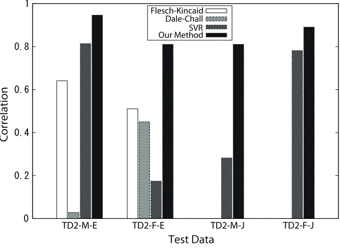
The TD2 data were sorted by the method explained in Section 3.2, and the correla-tion with the correct order was investigated. Three methods were used for comparison:
r
Flesch–Kincaidr
Dale–Challr
Support vector regression (SVR [Drucker et al. 1996])In these three methods, the readability level is obtained as a value, whereas our method presents an order. Therefore, the results of the three methods were sorted according to the values. The resulting orders for the three methods and for ours were then compared with the correct order in the test data. We used the finest annotation for correct ordering; for example, 27 levels for TD2-M-E, linear ordering for TD2-F-E, linear ordering for TD2-M-J, and 4 levels for TD2-F-J.
Here, SVR was trained by labeling the Time/Asahi newspaper texts as +1.0 and the texts ofTime/Asahifor children as –1.0, and then using the 600 texts for training. The LIBSVM package was used with the same kernel and parameter settings given in Section 6.
We used Spearman’s correlation to evaluate the ordering. Spearman’s basic correla-tion formula is
rs=1−
6ni=1d2i
n3−n
wherenis the number of texts, anddi is the difference in ranking between the correct
and obtained results for text i. This formula has an extended version to cope with multiple elements having the same ranking. Givenxandyas ordered sequences with the same ranking, the correlation is given as follows:
rs=
Tx+Ty−
n
i=1d2i
2TxTy
where
Tx=(n3−n)− nx
i=1
(t3i −ti), Ty=(n3−n)− ny
j=1
(t3j −tj)
Here,nx and ny are the numbers of the rankings for equivalently ranked elements in
x andy, respectively, andti,tj denote the number of elements with the same ranking
as elements which are indexed as i,j, respectively. For example, given an order x = [1,2,3,3,4],nx =1, because only 3 had the same ranking,ti=2 fori= 1, because there
are two 3s.
Correlation
Test Data
TD2-M-E TD2-F-E TD2-M-J TD2-F-J Flesch-Kincaid
[image:17.486.56.395.66.314.2]Dale-Chall SVR Our Method
Figure 7
Correlation with the test data.
data, there are only two bars, because Flesch–Kincaid and Dale–Chall are inapplicable. Moreover, note that the vertical heights are comparable within a data set but not among data sets, because the number of levels for each data set is different.
Comparing within each block, our method performed better than any other, having a correlation of more than 0.8 for all cases. Flesch–Kincaid performed quite well, having a high correlation of more than 0.6 for the TD2-M-E data. The use of SVR was less effective, with the correlation being lower than that with our method. This shows that the performance of the regression method is limited, even with a machine learning method, when training data for two levels only are available. In contrast, our method shows that even with rough two-level training data, high correlation is achievable. Such performance is enabled by comparison among texts even in the middle range between difficult and easy texts.
How this performance compares to that of previous classification methods is diffi-cult to say. Above all, our method cannot be fairly compared with previous classification methods from the viewpoint of classification, because in order to transform our sorted results into classes, we would have to give the number of texts in each class. Because this information is not provided to the classification methods, the comparison would be unfair, thus favoring our method. Therefore, the comparison must be made by means of correlation. Another problem is that because we do not possess the training data used in previous work, we could only test with what we have listed in Table 2.
correlation measured on sorted results. By exchanging the halves, the result reported here is the average of two-fold cross-validation.
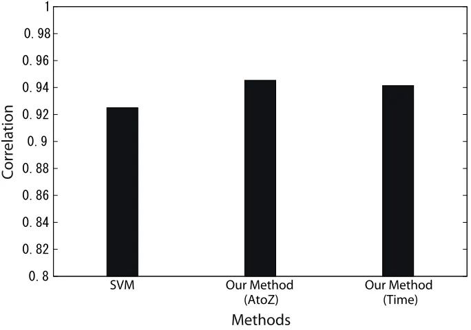
We compared three methods:
1. A classification method using part of TD2-E-M as training data.
2. The sorting method using the same part of TD2-E-M as training data.
3. The sorting method with TD1-E as training data.
The first classification method followed that of Schwarm and Ostendorf (2005). The amount of training data used to build a classifier foreachclass was 67 for +1 and 4×(67) for –1. The parameters used for the SVM were the same as those used for our method. For the second method, the training data consisted of 1,340 (2 ×5C2 [pairs among 5 classes]×67 texts) random pairs of two successive levels. Each fold of two-fold cross-validation was done five times by changing the pairs randomly. For the third method, TD1-E was used as in the previous evaluation, but this time the verification was done with five levels (whereas the first block in Figure 7 was evaluated with 27 levels). The amount of training data was the same as TD1 (i.e., 1,200) and the experiment was done five times by changing the pairs randomly.
The results are shown in Figure 8. Three bars are shown from first to third, cor-responding to each of the three methods. For classification, the correlation was 0.925, whereas the correlations of the second and third bars were 0.946, 0.941, respectively. Our methods thus slightly outperformed the classification method. Moreover, the difference between the second and third methods showed that two-level training data could perform similarly to multiple-level training data. This shows the strength of our method
Correlation
Methods
SVM Our Method(AtoZ)
[image:18.486.50.392.396.636.2]Our Method (Time)
Figure 8
in that it cancomplementa limited amount of training data through relative comparison within the set.
It is not our intention, though, to assert that our method is better than the classifica-tion method based only on this experiment. Classificaclassifica-tion has a much better chance of achieving better performance with large-scale training data, especially when features are studied further. The point here is to show the potential of the sorting model, especially when sufficient amounts of corpus data annotated in multiple classes are unavailable.
Finally, we investigated the effect of the amount of training data as mentioned in Section 3.1. Given a set of relatively difficult texts Ld and a set of easy texts Le, the
maximum number of training pairs will amount to 2× |Ld| × |Le|, with|L|indicating
the number of elements in set L. Two effects related to the amount of data should be considered. First, there is the effect of the absolute amount of data used; that is, the amounts of|Ld|and|Le|. We letN=|Ld|=|Le|and measured the correlation shift
by changing N from 100 to 600. For each N, the number of training pairs was 2N, constructed by randomly samplingNdocuments fromLd andLeand formingNpairs,
and then constructingVdeandVedfor each pair.
Second, the effect of combination should be considered; that is, the number of pairs whose maximum number is 2× |Ld| × |Le|for a givenN. WhenN= 600, this amounts
to 720,000 training pairs, which is too large in terms of the time required for training. Therefore, by fixingN= 100, we tested the learning effect for numbers of training pairs up to 2×100× {1, 5, 10, 50, 100}.
The results are shown in Figure 9, where the first graph shows the effect of the amount of data and the second graph shows the effect of combination. The horizontal axes represent the amount of training data (namely, 2Nfor the first graph and 2×100× {1, 5, 10, 50, 100}for the second graph), and the vertical axes represent the correlation. In the second graph, the horizontal axis is in log scale. Each graph has four lines, each corresponding to a subset of data from TD2. Every plot was obtained by averaging five repetitions of the random pairing of learning data.
In the first graph, the increase in the amount of local data led to only a slight increase in performance, which is almost invisible. In the second graph, the increase in combination did not lead to higher performance, but rather to drastically decreased performance for the English data. This decrease was especially prominent with TD2-F-E, the English textbook for Japanese students. This must have been due to the different natures of the training and test data. On the other hand, the texts of theAsahinewspaper articles and TD2-{M,F}-J are controlled under a similar standard (in terms of vocabu-lary, syntax, and so forth), which would account for the difference from the case in English.
These results suggest that even if our method has the possibility of obtaining large amounts of training data by combination, this would not lead to higher performance. Moreover, the graphs suggest the importance of obtaining a sufficient amount of train-ing data from two levels which match the target domain.
9. Evaluation of the Terrace System 9.1 Evaluation of Searching
TD2-M-E TD2-F-E TD2-M-J TD2-F-J
Correlation
Data Amount
Correlation
[image:20.486.48.391.58.556.2]Data Amount
TD2-M-E TD2-F-E TD2-M-J TD2-F-JFigure 9
Effect of increasing the amount of data (left: corpus data amount; right: training data amount increased by combination).
between the resulting and correct positions was measured. This procedure was repeated for all texts of TD2, and the average difference was obtained. The finest levels for TD2 were used as the correct annotation. The execution was again performed five times by changing the random pairing within the training data.
The results are shown in Figure 10. The horizontal axis represents blocks of TD2 data, and the vertical axis represents the average locational error of searching divided by the total number of levels of each data. Unlike the correlation figures seen so far, the smaller the value of each result, the better the precision of the search results. As was the case in Figure 7, the heights of bars are comparable within a data block, whereas bars across blocks are not comparable because of the different numbers of levels.
Naturally, the results are reversed from those of Figure 7. Methods with higher performance in sorting had smaller errors. Overall, our method had the smallest errors among all methods.
Because Terrace is different from previous systems based on the absolute scores of Flesch–Kincaid or Dale–Chall, it was presented to several language teachers who originated the Terrace project (as mentioned in Section 5). They reacted positively to Terrace, even though the system does not show any absolute readability scores. There are two main reasons for the favorable response. First, as mentioned, because they need texts rather than scores, teachers liked the fact that Terrace returns texts directly without outputting the values. With previous systems, teachers themselves had to input one candidate text after another to find one of an appropriate level. Second, for for-eign language teachers, especially of languages other than English, scores are not well standardized, and teachers are often puzzled by some readability scores. The teaching levels do not necessarily correspond to standard school grades for natives. Therefore, they prefer that a system outputs texts directly as in Terrace, because this means they
Average Error of Search
TD2-M-E TD2-F-E TD2-M-J TD2-F-J
Test Data
[image:21.486.56.397.388.635.2]Flesch-Kincaid Dale-Chall SVR Our Method
Figure 10
do not have to interpret some score which is difficult to assess. Nevertheless, they found that the graphical indicators are helpful for locating themselves among numerous collections.
9.2 Response Time
In Section 4, qualitative analysis showed that a disadvantage of our model is the greater computational complexity in readability assessment. This section reports on the response time when using Terrace.
The response time of Terrace is determined by the addition of three factors:
r
extraction of features from a textr
searching for the text’s position within a text collectionr
system overhead time (server access, Web page generation, etc.)The time needed for feature vector construction is linear with respect to the text length. This process is conducted once before a search. The text’s position within the text collection is then searched for. Because comparison is performed multiple times in a search, this factor dominates the response time. As mentioned in Section 3.2, this time is logarithmic with respect to the number of texts in a collection. The last factor is constant.
We evaluated the response time for TD2-M-E, since we currently have a larger text collection in English and TD2-M-E is a larger data set than TD-F-E. As noted in Section 5, this collection amounts to 14,877 texts taken from CNN (CNN 2008). The input texts were all texts of TD2-M-E. Because K=2, which makesM=2×K+1=5 (e.g., the width of comparison was 5), the total number of comparisons was about 70 for one search. The computational environment was as follows: CPU: Intel(R) Core(TM)2 Quad CPU Q9550 (2.83 GHz); main memory: 3.5 GB; OS: Debian GNU/Linux 4.0.
The results are plotted in Figure 11. Because the key factor for response time is the length of a text, the horizontal axis represents the text length and the vertical axis represents the response time. Each plot corresponds to one text in TD2-M-E. The longer the text, the slower the response time will be. The plotted points are separated into two clusters, with one at the upper right and the other just below. This disjunction corresponds to texts which were judged as more difficult and those judged as easier, respectively, at thefirstcomparison within the binary search. Because the Terrace system stores its feature vectors in a MySQL database, when the number of non-zero features is large, access becomes slower, even when all vector dimensions are the same. For texts judged as more difficult at the first comparison, the vector length in the string (which is how it is implemented in MySQL) becomes longer, and the overall procedure takes a longer time. In any case, for all texts the response time was less than a second. Therefore, although our method does have a complexity disadvantage, the results of this evaluation suggest this is not a serious problem.
10. Conclusion
Response Time (s)
[image:23.486.57.391.67.310.2]Number of Words
Figure 11
System response time for texts in TD2-M-E.
compared to other texts, rather than based on an indicator of the absolute difficulty of the text. In our method, a comparator is constructed using an SVM, which judges which of two texts is more difficult. This comparator is then used to sort the texts of a given set using a binary insertion sort algorithm. Our method differs from traditional readability assessment methods, most of which are based on linear regression, and it also differs from recent methods of statistical readability assessment, which are based on multi-value classification. The advantage of our model is that it solves the problem of assembling training data annotated in multiple classes, because it only requires two classes of training data: easy and difficult. At the same time, our model has the disadvantages of the resulting norm being somewhat incomprehensible as a ranking and greater computational complexity compared to previous methods.
After performing a fundamental evaluation, we compared the overall performance of our method with those of other methods. Our method achieved a higher correlation with the gold standard, more than 0.8, in sorting text collections in both English and Japanese; this was higher than both traditional methods and an SVR trained with two-class corpora. Another comparison with a state-of-the-art classification method confirmed the potential of our method.
We also presented an actual application, called Terrace: a system that retrieves a text of similar readability from a text collection when given an input text. We showed that Terrace can overcome the disadvantages of the proposed model, by introducing a graphical representation of the positions of texts with known levels, and also by verifying that the response time is always less than a second.
References
Alderson, J. C. 1984.Reading in a Foreign Language: A Reading Problem or a Language Problem. London; New York: Longman. Amano, S. and T. Kondo. 1995. Modality
dependency of familiarity ratings of Japanese words.Perception & Psychophysics, 57(5):598–603. Amano, S. and T. Kondo. 2000. On the
NTT psycholinguistic databases ‘lexical properties of Japanese’.
Journal of the Phonetic Society of Japan, 4(2):44–50.
AsahiNewspaper. 2008.http://www. asahi.com/, accessed in June 2008. Barzilay, R. and M. Lapata. 2008. Modeling
local coherence: An entity-based approach.
Computational Linguistics, 34(1):1–34. Chall, J. S. and E. Dale. 1995.Readability
Revisited: The New Dale–Chall Readability Formula. Cambridge University Press, Cambridge.
Chang, C. and C. Lin. 2001.LIBSVM: A Library for Support Vector Machines. Software available athttp://www. csie.ntu.edu.tw/∼cjlin/libsvm. CNN. 2008.http://edition.cnn.com,
accessed in September 2008.
Cohen, W. W., R. E. Schapire, and Y. Singer. 1998. Learning to order things.Journal of Artificial Intelligence Research, volume 10, pages 243–270.
Collins-Thompson, K. and J. Callan. 2004. A language modeling approach to predicting reading difficulty. In
Proceedings of HLT–NAACL, pages 193–200, Boston, MA. Database, MRC Psycholinguistic. 2006.
http://www.psy.uwa.edu.au/ mrcdatabase/uwa mrc.htm, accessed in December 2006.
Drucker, H., Burges C., J. C. Kaufman, A. J. Smola, and V. Vapnik, 1996.
Support Vector Regression Machines. MIT Press, Cambridge, MA. DuBay, W. H. 2004a.The Principles of
Readability. Impact Information, Costa Mesa, CA.
DuBay, W. H. 2004b.Unlocking Language: The Classic Studies in Readability. BookSurge Publishing, Charlestown, South Carolina. Inui, K. and S. Yamamoto. 2001.
Corpus-based acquisition of sentence readability ranking models for deaf people. InNatural Language Processing Pacific Rim Symposium, pages 205–212, Tokyo, Japan. JEES. 2008. Japanese Proficiency Test
http://www.jees.or.jp/jlpt/en/
provided by Japanese Educational Exchange and Services, accessed in November 2008.
Joachims, T. 1998. Text categorization with support vector machines. In
European Conference on Machine Learning, pages 137–142, Chemnitz, Germany. Joachims, T. 1999. Making large-scale
support vector machine learning practical. In Bernhard Sch ¨olkopf, Christopher J. C. Burges, and Alexander J. Smola, editors,
Advances in Kernel Methods: Support Vector Learning. MIT Press, Cambridge, MA, pages 169–184.
Joachims, T. 2002. Optimizing search engines using clickthrough data. InInternational Conference on Knowledge Discovery and Data Mining, pages 133–142, Edmonton, Alberta, Canada.
Kincaid, J. P., R. P. Fishburne, and R. L. Rodgers. 1975. Derivation of new readability formulas for Navy enlisted personnel. Research Branch Report 8–75, U.S. Naval Air Station.
Klare, G. R. 1963.The Measurement of Readability. Iowa State University Press, Ames.
KodomoAsahi. 2008. Asahi Newspaper for Junior School Students.http://www. asagaku.com/, accessed in June 2008. Kudo, T. 2009. Mecab, yet another
part-of-speech and morphological analyzer. Available from
http://mecab.sourceforge.net/. Laufer, B. 1991.How Much Lexis is Necessary
for Reading Comprehension? Vocabulary and Applied Linguistics. Macmillan, Basingstoke.
Miyaji, H. 2008.Junior and Junior High School Japanese. Mitsumura Tosho, Tokyo. From the 3rd grade to the 9th grade, in Japanese.
Morizumi, M. 2007.New Crown English Series 1, 2, 3. Sanseido, Tokyo.
Paice, C. and G. Husk. 2008. The lancaster stemming algorithm. Available from http://www.comp.lancs.ac.uk/ computing/research/stemming/ index.htm.
Pitler, E. and A. Nenkova. 2008. Revisiting readability: A unified framework for predicting text quality. InProceedings of EMNLP, pages 186–195, Honolulu, Hawaii.
ReadingA-Z.com. 2008. Reading A–Z Leveling and Correlation Chart
Schwarm, S. E. and M. Ostendorf. 2005. Reading level assessment using support vector machines and statistical language models. InAnnual Meeting of the ACL, pages 523–530, Ann Arbor, Michigan. Si, I. and J. Callan. 2001. A statistical model
for scientific readability. InCIKM, pages 574–576, Atlanta, Georgia. Tanaka-Ishii, K. and H. Terada. 2009. Word
familiarity and frequency.Studia Linguistica. accepted in 2009, in press, to appear in 2010.
Time. 2008.http://www.time.com, accessed in July 2008.
TimeForKids. 2008.http://www. timeforkids.com/, accessed in August 2008.
Washburne, C. and M. Vogel. 1928.Winnetka Graded Book List. Chicago, American Library Association.
Xia, F., T. Liu, J. Wang, W. Zhang, and H. Li. 2008. Listwise approach to learning to rank: theory and algorithm. In
International Conference on Machine Learning, pages 1192–1199, Helsinki, Finland.