Comparative analysis of the food and nutrients demand in developing countries: The case of main vegetable products in South Asian countries 

Demand for food is a field that has encouraged much activity in economic research and has a long history within the economics profession. At least, ever since Malthus (1798), there has been a recur-ring focus on the availability of food. The particular concern of Malthus was that the growth in population would eventually produce demands for food exceed-ing supply. Approximately 309 million of around 850 million undernourished people in the world live in India, Pakistan and Bangladesh, according to the State of Food Insecurity in the World (SOFI 2011). Therefore, these countries are much concerned by this problem.

According to the SOFI (2011), prices of food com-modities in the world markets, adjusted for inflation, declined substantially from the early 1960s to the early 2000s, when they reached a historic low. They increased slowly from 2003 to 2006 and then surged upwards from 2006 to the middle of 2008 before declining in the second half of that year. According to the UNCTAD database, in the current US dollars, world prices for main grains and oilseed products surge again in 2010 and 2011 and got their highest historical levels notably for wheat, maize and soy-beans products. A number of articles analyzed the

reasons of these evolutions (Gomez 2008; Trostle 2008; Laap1990; Carrasco et al. 2012). Generally, the main reasons presented for the price inflation are the strong global growths in the average income combined with the rising population, which has increased the demand for food, particularly in developing coun-tries, over the last decades. Other factors that have added to the global food commodity price increase include, at the structural level, the declining value of the local currency compared to the US dollar, the rising energy prices, the diminution of research in the agricultural field, the development of bio fuels and some more conjectural reasons: the drop of some crops productions due to the climatic problems, in-terventions of some governments to control imports or exports, speculation in the world markets. Some studies emphasize more precisely on the local condi-tions and interrelacondi-tionships between the world and the South Asian markets evolution (Carrasco et al. 2012; World Bank South Asian region 2010).

The prevailing source of the insufficient food con-sumption in developing countries is the lack of access due to the low income (World Bank 1981), although it is not the only cause according to the SOFI (1999). Therefore, the effect of income and price on the

de-Comparative analysis of the food and nutrients demand

in developing countries: The case of main vegetable

products in South Asian countries

Muhammad Rizwan Yaseen

_{, Irfan Mehmood}

_{, Qasim Ali}

1_{Government College University, Faisalabad, Pakistan}

2_{Pakistan Agricultural Research Council, Faisalabad, Pakistan}

Abstract: Being the most populous countries of South Asia, India, Pakistan and Bangladesh together represent about 37%

of the world total undernourished population. In the article, there are calculated the expenditure elasticities and the own and cross non-compensated price elasticities of main vegetable products of these countries by using the LA-AIDS model. Th ere are used the elasticity estimates to decompose the recent demand fl uctuations into price eff ect, income eff ect and population eff ect for each country. Th en the ways for the government to improve the protein and energy intake after cal-culating the vegetable protein and calories elasticities are compared. Wheat and rice in these countries are relatively price inelastic. For these three countries, the population development (as well as the revenue for India and Bangladesh) appears to be the most important and regular cause of the augmentation of demand for vegetable products. A combination of in-come and price policies may be more eff ective in infl uencing the consumption pattern. Th e government should aim at im-proving the income level of most vulnerable consumers (low income group) in these countries.

Key words: amelioration, expenditure elasticities, LA/AIDS, price elasticities, protein and calorie intake, vegetal food

mand for food in developing countries has been the focus of many studies; see e.g. (Mellor 1983; Behrman and Deolalikar 1987; Alderman 1988).

In this paper, our objective is to analyse the vegeta-ble food consumption pattern and its response to the changes in expenditures and prices for Pakistan, India and Bangladesh, which share a colonial past and are currently the low or middle income level countries at different stages of economic development. The calculation of expenditure and prices elasticities ma-trices for vegetable products is a stage in our project to estimate both the animal and vegetable products demands with a two stage budgeting method and put them in relation with the supply elasticities that we have already calculated (Yaseen et al.2011a, b). So we would be able to construct a partial equilibrium model for each country and make scenarios for 2020.

There exists some data on the matrix demand elas-ticities for these countries in the literature but they are generally badly documented (Food and Agricultural Policy Research Institute) or old, they took both vegetable and animal products (and some non-food products) or they are calculated for a specific year using the panel data. So we decided to use the time series data to calculate elasticities and their decom-position into the rice effect as well as the income effect. For attaining this objective, we had to do some approximations, notably because the retail prices are generally not present in the international databases.

This kind of results (elasticities) is essential to es-timate the future demand of agricultural products to attain food security in these countries. This study is an attempt towards this direction, with the focus on the estimation of the demand parameters of major vegetable food commodities. A better understand-ing of demand elasticities helps to predict the future demand of food products under different scenarios of prices and income and could prove worthy for the policy planners on important policy decisions.

METHODOLOGY

We used the linear approximation version of the AIDS model (proposed by Deaton and Muellbauer 1980a, b) called the LA/AIDS employed by Alderman (1988), based on a particular form of the cost function (or expense) belonging to the class “Price Independent

Generalized Logarithm” (Holt and Goodwin 2009). Following the classical method, we have estimated the

n – 1 share equations ݏ௜ൌ ݌݅ ൈ

ݔ݅

ܯ of the n products for

utility maximizing agents (Holt and Goodwin 2009):

ݏ௜ൌ Ƚ௜൅ ෍ ɀ௜௝Ž݌௝ ௡

௝ୀଵ

൅ Ⱦ௜Ž ܯ

ܲ

i = 1, 2, …, n – 1 j = 1, 2, …, n (1)

where p_j is the price for each product, M the total

expense per capita for the products taken into

ac-count and P is a price index defined by

Žܲ ൌ ෍ ݏ௝ൈ Ž݌௝ ௡

௝ୀଵ

(2)

The linear homogeneity of cost function, the sym-metry of the second-order derivatives, and adding up across the share equations implies the following set of restrictions:

෍ Ƚ௜ൌ ͳ ௡

௜ୀଵ

ǡ ෍ ɀ௜௝ ௡

௜ୀଵ

ൌ ෍ ɀ௜௝ൌ Ͳǡ ௡

௝ୀଵ

෍ Ⱦ௜ ௡

௜ୀଵ ൌ Ͳ

ɀ_௜௝ൌ ɀ_௜௝ (3)

The elasticities are calculated by the following

ex-pressions where ݏҧ௜ and ݏҧ௝ are the mean of the share

on the whole period of the estimation:

(1) for the Marshallian1 _{(or uncompensated)}

elas-ticity of the product i consumption relative to the

price of the product j:

Marshallianelasticity = ܧ_௜௝ெൌ െɁ௜௝൅ ɀ_௜௝

ݏҧ௜ െ Ⱦ௜

ݏҧ_௝ ݏҧ௜

(4)

Where δ_ij is the Kronecker delta term (that is 1

when i = j or 0 when i ≠ j)

(2) for the expenditure elasticity of the product i

consumption

Revenue elasticity = ܧ_௜ோൌ ͳ ൅ Ⱦ௜ ݏҧ௜

(5)

From the calculated elasticities for the different vegetal products, it is also possible to calculate the

different elasticities for different nutrients (N =

pro-tein or calorie) demands relative to the price of the

product j:

1_{The Marshallian demand function simply shows the relationship between the price of a good and the quantity demanded}

ܧ_௝ேൌ ෍ሺݍ௜ൈ ܺ௜Τ ሻ ൈ ߲Žܺܳ ௜Τ߲Ž݌௝ ௡

௜ୀଵ

(6)

where q_i is the content in the considered nutrient

in the product i (in grams of protein or calories per

1 gram of product), x_iis the amount of the product i

consumed per capita and per day and Q is the amount

of protein (or calories) given by all vegetable foods, including those not taken here.

With r_i = q_i × x_i/Q, that is the share of the total

vegetable proteins (or vegetable calories) given by

the product i, we have

ܧ_௝ேൌ ෍ ݎ௜ൈ ܧ௜௝ ௡

௜ୀଵ

(7)

E_ij is the Hicksian or Marshallian elasticity of the

ith _{product relative to the price of j}th _{product. The}

same calculations can be made for the nutrient rev-enue elasticities:

ܧܴே_{ൌ ෍ ݎ} ௜ൈ ܧ௜ோ ௡

௜ୀଵ

(8)

where ܧ_௜ோ _{is the revenue elasticity of the product i.}

The data (consumption and price) used in the LA/AIDS model for the three countries are taken from the FAOSTAT database. Regarding the food taken into account, we selected seven product families, including three individual products (rice, wheat, maize), two products together (millet/sorghum) and three families of products (pulses, sugar and sweeteners, vegetable oils). Concerning prices, the database provides only the producer prices for rice, wheat, millet/sorghum, sugar cane, and pulses. We had the effective retail prices data of these all products for some years so we used a corrective multiplicative factor to apply

to each series of producer prices such that the mean for the available years of the retail price is equal to the mean of the “corrected producer price”. We made some more estimations and approximations

concern-ing sugar, vegetable oils and millet/sorghum2_.

It is important to notice that due to the linearity in prices of the share equations defined in the Equation (6), the fact to use producer prices instead of consumer prices has no influence on the prices and expenditures elasticities as far as those two set of prices evolve in parallel. This is an important not demonstrated hy-pothesis 3, but it is necessary to perform the estima-tions in time series. The LA/AIDS model estimated a system of six (or five) equations with seven (or six) products for each country (in each case wheat has been removed from the system). The FIML (Full Information Maximum Likelihood) method ensures that the coefficients of the equations are independent of the equation which is not taken into account. The coefficients of this excluded equation are estimated by taking into account the fact that the sum of the share of expenditure for all the products is equal to one.

It is conventional to introduce some “dummy vari-ables” that are intended to counteract the problems (economic events unrelated to changes in prices and expenditures, and even the presence of some

unreli-able data or outliers)4_{. The lack of reliable data is a}

major problem in econometric research concerning the less-developed countries, as the time series analysis requires consistent data for a reasonable time span, which often is not available for these countries.

Analysis of main results

The results of the estimations for three counties are indicated in Tables 1 to 5.

2_{For sugar, the producer price was not available in the FAOSTAT, so we selected the price of sugarcane divided by 0.08}

(the average yield of 8% sugar in sugar cane according to the Pakistan Sugar Mills Association). For vegetable oils, the FAOSTAT does not provide any price. Given the growing importance of the palm oil, the price for this product was calculated, based on the FAOSTAT data of foreign trade, the unit values of imports (imports in value divided by im-ports in quantity). Where possible, we performed the same calculations for the imim-ports of soybean and rapeseed oils. These values are only available for some years, so we calculated regression equations of the price for each of these oils based on that of the palm oil and supplemented the missing price data with the equations. We calculated the weighted average unit values of these three products and then converted them into the local currency. For the category millet/ sorghum, the price was taken as the average price of each product weighted by the respective share of consumption of these products in the total consumption of both products.

3_{However, where data is available, we can observe a high correlation coefficient between the retail and producer prices,}

and a graphically simultaneous evolution, mainly for the crops but also to some extent for sugar and vegetal oils.

4_{However, despite the presence of these variables, the mainstreaming of seven product families for India and Bangladesh}

T

able 1. Co

ef fi cien ts of shar e s e q ua tions f or Pak ist

an, India and B

anglade sh     R ic e Mai ze Mille t/s or gh um Sug a r V e g e tal oils D ry b e an Pak ist an India B angla- de sh Pak ist an India B angla- de sh Pak ist an India B angla- de sh Pak ist an India B angla- de sh Pak ist an India B angla- de sh Pak ist an India B

angla- desh

Const an t 0.46*** 0.97*** 1.08** 0.08 –0.02 0.01 0.29*** –0.15 0.02 –0.44* 0.54*** 0.06 –1.2*** 0.18 –0.11 0.58*** (0.18) (0.33) (0.42) (0.07) (0.07) (0.03) (0.06) (0.21) (0.01) (0.25) (0.18) (0.15) (0.30) (0.14) (0.2) (0.18) Ri ce 0.09*** 0.26*** 0.11*** –0.007 –0.005 –0.001 –0.001 –0.008 –0.001* 0.007 –0.05*** –0.02*** –0.01 –0.05*** –0.02** –0.007 (0.02) (0.02) (0.02) (0.005) (0.003) (0.002) (0.004) (0.01) (0.001) (0.01) (0.009) (0.008) (0.01) (0.007) (0.01) (0.01) Mai ze –0.008 –0.06** –0.001 0.01*** 0.01** 0.0002 –0.003 –0.02* 0.0004 –0.0003 –0.01 –0.0003 –0.004 –0.001 –0.00006 –0.008 (–0.006) (–0.03) (–0.002) (0.005) (0.005) (0.001) (0.002) (0.01) (0.0003) (0.01) (0.01) (0.002) (0.002) (0.01) (–0.001) (0.006) Mille t/ so rg h u m –0.001 –0.02 (–0.002* –0.003 –0.001 0.0005 0.01*** 0.05*** –0.0007 0.01** 0.003 –0.001* 0.001 –0.01* 0.0001 –0.01** (–0.004) (–0.01) (–0.001) (0.002) (0.002) (0.0003) (0.002) (0.008) (0.001) (0.003) (0.007) (0.001) (0.003) (0.005) (–0.0004) (–0.004) Sug a r 0.007 (–0.06*** –0.02*** –0.0003 –0.008** –0.0003 0.01** –0.008 –0.001* 0.04*** 0.10*** 0.04*** –0.06*** –0.01** –0.0007 0.001 (–0.01) (–0.01) (–0.008) (0.006) (0.003) (0.002) (0.004) (0.008) (0.001) (0.02) (0.007) (0.007) (0.01) (0.005) (–0.005) (–0.01) V e ge ta ble oils –0.01 –0.04*** (–0.02** –0.004 –0.0004 –0.00006 0.001 –0.0001 0.0002 –0.06*** –0.02*** –0.0007 0.10*** 0.08*** 0.02*** 0.002 (–0.01) (–0.01) (–0.009) (0.003) (0.002) (0.001) (0.003) (0.007) (0.0005) (0.01) (0.007) (–0.004) (0.01) (0.005) (–0.006) (–0.007) Whe at –0.07 –0.08*** –0.06*** 0.01 –0.005 0.0005 –0.01** –0.04*** 0.003* –0.01 –0.03* –0.02** –0.02** 0.014 0.001 –0.03*** (0.01) (0.03) (0.07) (0.007) (0.005) (0.002) (0.004) (0.02) (0.002) (0.01) (0.01) (0.007) (0.01) (0.01) (–0.007) (–0.01) Dr y b e ans 1 –0.007 –0.01 –0.009** 0.001 0.001 0.05*** (0.01) (0.006) (0.004) (0.01) (0.007) (0.01)

  Lag (1)

0.37*** –0.1 0.04 0.39*** –0.06 1.24*** 0.15* 0.05 0.56*** 0.24*** –0.15*** 0.50*** 0.02 0.09** 0.19* 0.2** (0.07) (0.06) (0.10) (0.12) (0.15) (0.07) (0.08) (0.07) (0.14) (0.08) (0.05) (0.08) (0.007) (0.038) (0.11) (0.07)

Log (ex

p endit ur e) –0.08 –0.08 –0.04 –0.01 0.01 –0.002 0.06*** 0.05 –0.003 0.13** –0.07** –0.01 0.25*** –0.04 0.02 –0.11*** (0.03) (0.06) (0.07) (0.01) (0.01) (0.007) (0.01) (0.03) (0.002) (0.05) (0.03) (0.03) (0.06) (0.02) (0.03) (0.03) R 2 0.87 0.93 0.7 0.73 0.89 0.93 0.85 0.88 0.6 0.66 0.92 0.7 0.85 0.93 0.74 0.86 R

2 a

just 0.83 0.9 0.6 0.65 0.85 0.91 0.8 0.83 0.5 0.56 0.89 0.58 0.8 0.90 0.66 0.81 DW 1.12 1.30 1.72 1.97 1.43 1.49 0.71 1.41 2.2 1.04 1.04 1.7 0.81 0.77 2.04 1.61

DW = D

urbin-W

at

son; (*), (**) and (***) r

e pr e sen t t he le ve

l of sig

nif

ic

anc

e a

t 10%, 5% and 1%

1dr y b e ans ar e  us ed  a s a  sy non y m  of  pu ls es S our

ce: our e

stima

Table 1 shows the coefficients of the six (or five) equations of the LA/AIDS model for Pakistan, India and Bangladesh, respectively. We also introduced a lagged variable to correct the autocorrelations between the years. The significances of different parameters at the probability levels of 10%, 5% and 1% are indicated on this table by one star (*), two stars (**) and three stars (***), respectively.

Considering the R2 _{adjusted values and the}

signifi-cance of main coefficients, our results are satisfac-tory. Concerning the Durbin-Watson, the values are generally near to 2 and always superior to 1.1 except for millet/sorghum for Pakistan as well as vegetable oil for Pakistan and India.

The coefficients of the lagged expenditure share appearing in Table 1 are generally significant and important, which indicated high “memory effects”,

that is the food consumption in year t is influenced by the consumption during the preceding years. When the coefficient of the lagged variable in the share equation is positive, the long term elasticities are greater than the short term elasticities (this is generally the case and the multiplicative coefficient can be important).

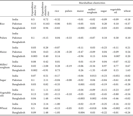
The expenditure elasticities are indicated in Table 2. They are generally positive (normal goods) and the higher values are for sugar in Pakistan (2.11), for wheat in India (2.15) and Bangladesh (1.48). These clearly indicate that, when the revenues (expenses for vegetal food products) increase, the Indian and Bangladeshi people consume first more wheat (which is an appreciated cereal allowing a diversification from rice) and more vegetable oils, sugar and rice, but less subsistence food such as maize and millet/

Table 2: The expenditure and the Marshallian elasticities

E

x

p

endit

ur

e

shar

e (%)

E

x

p

endit

ur

e

el

a

sticity

ri

ce

Marshallian elasticities

rice pulses maize _sorghummillet/ sugar vegetable _oil wheat

Rice 

India 0.5 0.72 –0.32   –0.01 –0.02 –0.09 –0.09 –0.18

Pakistan 0.15 0.163 –0.06 0.01 –0.05 0.01 0.20 0.10 –0.37

Bangladesh 0.83 0.94 –0.82 –0.001 –0.002 –0.03 –0.03 –0.062

Pulses 

India              

Pakistan 0.1 –0.15 0.04 –0.33 –0.05 –0.07 0.18 0.30 0.10

Bangladesh              

Maize

India 0.03 0.28 –0.07   –0.11 0.03 –0.23 –0.11 0.21

Pakistan 0.04 0.63 –0.28 –0.28 –0.47 –0.09 0.04 –0.09 0.54

Bangladesh 0.003 0.40 0.14   –0.94 0.15 0.04 0.007 0.20

Millet/ sorghum

India 0.08 0.42 0.01   0.01 –0.19 0.04 –0.07 –0.22

Pakistan 0.02 –2.08 0.28 –0.19 –0.06 –0.34 0.97 0.77 0.67

Bangladesh 0.002 –0.91 0.73   0.26 –1.35 –0.49 0.15 1.63

Sugar

India 0.07 0.51 –0.17   –0.04 0.013 –0.23 –0.051 –0.02

Pakistan 0.1 2.11 –0.04 –0.08 –0.02 0.04 –0.84 –0.61 –0.30

Bangladesh 0.03 0.82 –0.33   0.001 –0.02 –0.19 –0.01 –0.28

Vegetable oils

India 0.1 1.11 –0.52   –0.04 –0.09 –0.15 –0.23 –0.07

Pakistan 0.13 1.83 –0.15 –0.10 –0.05 –0.02 –0.45 –0.80 –0.54

Bangladesh 0.04 1.48 –0.94   –0.003 0.002 –0.04 –0.46 –0.02

Wheat

India 0.24 2.14 –1.00   –0.02 –0.19 –0.25 –0.16 –0.52

Pakistan 0.5 0.68 –0.15 –0.05 0.03 –0.018 0.06 –0.002 –0.55

Bangladesh 0.09 1.48 –1.05   0.004 0.03 –0.22 –0.01 –0.24

sorghum. Millet/sorghum and pulses are the “inferior good” in Pakistan (elasticities –2.09 and –0.15). This could be explained by the fact that in these countries, more population lives in rural areas and when the expenditure increases, then the rural people preferred to buy animal products as the protein source, while all the vegetable products are normal goods in India.

Elasticities are important parameters widely used in empirical works with agricultural models. In the general literature, all results available are calculated

globally for the vegetable and animal products (some-times also for the non-food products), so the com-parisons of values for the price (the share for each product is very different) and revenue (it refers to only vegetable food expense in our estimation and to the whole expense in other studies) elasticities are not pertinent.

The Table 2 also expresses the Marshallian elastici-ties for seven (or six) products (rice, maize, millet/ sorghum, sugar, vegetal oil, wheat and pulses) of India,

Table 3. Protein and caloric intakes in 2007 for Pakistan, India and Bangladesh

PROTEINS

Pakistan  India  Bangladesh

g/capita/day repartition (%) g/capita/day repartition (%) g/capita/day repartition (%)

Total proteins 59.2 100.00 57.4 100.00   50.5 100.00  

Animal products 23.5 39.70 10.2 17.80   7.8 15.40  

Vegetable products 35.7 60.30 100.00 47.2 82.20 100.00 47.2 93.50 100.00

Seven main vegetal

products 31.9 54.00 89.40 40.6 70.70 86.00 38.2 75.60 80.90

Wheat 22.00 61.60 15.00 31.80 3.7 7.80

Rice (milled

equivalent) 2.8 7.80 13.2 28.00 29.9 63.30

Maize 1.8 5.0 1.2 2.50 1.7 3.60

Millet/sorghum 0.4 1.1 3.8 8.10 0.0 0.00

Sugar (total) 0.1 0.3 0.1 0.20 0.1 0.20

Pulses (total)) 4.7 13.2 7.3 15.50 2.8 5.90

Vegetable oils (total)) 0.1 0.3 0.00 0.00 0.0 0.00

CALORIES

Pakistan  India  Bangladesh

kcal/capita/

day repartition (%)

kcal/capita/

day repartition (%)

kcal/capita/

day repartition (%)

Total calories 2 293.00 100.00 2 352.00 100.00   2 281.00 100.00  

Animal products 468.00 20.40 197.00 8.40   83.00 96.40  

Vegetable products 1 825.00 79.60 100.00 2 155.00 91.60 100.00 2 198.00 3.60 100.00

Seven main

vegetable products 1 658.00 72.30 90.80 1910.00 81.20 88.60 2 055.00 90.10 93.50

Wheat 843.00 46.20 514.00 23.90 126.00 5.70

Rice (milled

equivalent) 148.00 8.10 703.00 32.60 1 591.00 72.40

Maize 65.00 3.60 47.00 2.20 62.00 2.80

Millet/sorghum 15.00 0.80 131.00 6.10 1.00 0.00

Sugar (total) 262.00 14.40 193.00 9.00 79.00 3.60

Pulses (total) 77.00 4.20 122.00 5.70 45.00 2.00

Vegetable oils (total) 248.00   13.60 200.00   9.30 151.00   6.90

Pakistan and Bangladesh, respectively. Confirming to what was expected; the signs of direct price elastici-ties are always negative. The mean shares are also indicated in Table 2. Concerning the Marshallian own price demand elasticities in India, we observe that the absolute value is the highest for wheat (0.52), followed by rice (0.32), vegetal oil (0.25), sugar (0.24), millet/sorghum (0.19) and maize (0.11). This indi-cates that, when the expense for the vegetable food products is constant, people react highly and quickly to price changes for these two basis food products (wheat and rice). The Indian consumer is less reac-tive to the price of millet/sorghum and maize, which are more consumed on the farms. For Pakistan, the highest absolute value is for sugar (0.85), vegetable oil (0.80), wheat (0.55), maize (0.47), then millet/ sorghum (0.35), pulses (0.33) and rice (0.10). These figures show that the Pakistan consumers react highly to price changes mainly for wheat, vegetal oils and rice, but also for other products. For Bangladesh, the highest absolute value is for millet/sorghum (1.35), maize (0.94), rice (0.82), vegetable oil (0.47), pulses (0.33), wheat (0.24) and sugar (0.19).

Therefore, our results are different for each country, but rice, maize and wheat are price inelastic products in all countries (the level inferior to 1).The seven vegetable products taken into account in our analysis

represent an important share of the total protein and caloric intakes in the three countries (Table 3). Table 3 represents that wheat and rice are the major sources of protein and calories in these countries among all products analyzed here.

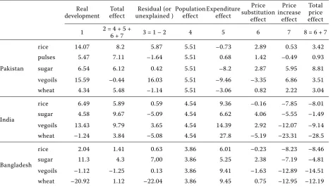
The demand elasticities allow us to determine the effects of different variables (demography, revenue, prices) on the evolution of consumption of these products (Table 4) during the crucial period 2006 to 2008 compared to the preceding years.

The main vegetable food products prices increased rapidly during the years 2006 to 2008, which was manifested by the fact that the consumer price index (CPI) by the World Bank dataset increased during these years by 31.3%, 25.5% and 18% in Pakistan, Bangladesh and India, respectively. In this period, the current gross domestic product increased, in the local currency units (LCU) by 47.8% in Pakistan (12.8% in constant LCU), 37.5 in Bangladesh (15.8% in constant LCU) and 46.8% (22.5% in constant LCU) in India. Using the calculated elasticities matri-ces presented previously, we can explain the most important evolutions of the total consumption of main vegetable foods in these countries during this period (2002–2005 and 2006–2008) and to decom-pose them for each country in four effects; (1) the population effect, (2) the expenditure effect (more

Table 4. Decomposition of the recent demand development into the price, revenue and population effects (be-tween 2002–2005 and 2006–2008) in %

Real development

Total effect

Residual (or unexplained )

Population effect

Expenditure effect

Price substitution

effect

Price increase

effect

Total price effect

1 2 = 4 + 5 + _{6 + 7} 3 = 1 – 2 4 5 6 7 8 = 6 + 7

Pakistan

rice 14.07 8.2 5.87 5.51 –0.73 2.89 0.53 3.42

pulses 5.47 7.11 –1.64 5.51 0.68 1.42 –0.49 0.93

sugar 6.54 6.12 0.42 5.51 –8.2 2.87 5.95 8.81

vegoils 15.59 –0.44 16.03 5.51 –9.46 –3.35 6.86 3.51

wheat 4.34 5.48 –1.14 5.51 –3.06 0.82 2.22 3.04

India

rice 6.49 5.89 0.59 4.54 9.36 –0.16 –7.85 –8.01

sugar 4.58 9.67 –5.09 4.54 6.62 4.06 –5.55 –1.49

vegoils 13.43 9.79 3.65 4.54 14.39 2.92 –12.07 –9.14

wheat –1.24 3.84 –5.08 4.54 27.8 –5.19 –23.31 –28.5

Bangladesh 

rice 2.04 1.41 0.63 3.86 6.01 –0.23 –8.23 –8.46

sugar 11.3 4.3 7,00 3.86 5.25 2.38 –7.19 –4.81

vegoils –1.12 –1.25 0.13 3.86 9.41 –1.63 –12.89 –14.51

wheat –20.92 1.12 –22.04 3.86 9.45 0.75 –12.95 –12.19

T

able 5. Co

st

s of im

pr ov ing t he n utr ien ts in ta ke s

Subsidy on one product

Consum ption of e a ch cr op Pr ic e E x p endit ur e on e a ch cr op Sub sidy

(1% of e

ach cr op ex p endit ur e ) Pr ot ein el a sticity C alor ie el a sticity Pr ot ein ef fe c t C alor ic ef fe c t Co st t o add one g ram pr ot ein Co st t o add 100 c alor ie s 1 2

3 = 1 × 2

4

= 3 × 0.01

5

6

7 = ve

ge

ta

ble

pr

ot

ein × 5

8 = ve

ge ta l c alor ie

s × 6

9 = 4/7

10 = 8/7

U nit s kg/he ad/ye ar LC U/kg LC U/he ad/ye ar LC U/he ad/ye ar g/he ad/da y C al/he ad/da y LC U/he ad/ye ar LC U/he ad/ye ar Pak ist an ri ce 17.14 48.62 833.3 8.33 –0.013 –0.013 0.04 1.95 235.2 426.63 puls e s 5.5 198 1 088.58 10.89 0.02 0.006 –0.09 –0.49 –115.73 –2 236.06 mai ze 8.24 74.12 610.91 6.11 –0.032 –0.023 0.06 1.5 108.02 407.62 mill/s or g 1.62 27 43.78 0.44 0.023 0.017 –0.01 –0.24 –48.56 –179.59 sug ar 27.65 27 746.62 7.47 –0.006 –0.264 0 69.42 12 667.57 10.76 ve goils 12.3 50.62 622.46 6.22 –0.006 –0.288 0 71.38 9 162.07 8.72 whe at 108.66 28.75 3 123.87 31.24 –0.422 –0.316 9.28 266.84 3.37 11.71 India   ri ce 108.68 24.5 2 662.6 26.63 –0.202 –0.236 2.67 165.52 9.96 16.09 mai ze 5.76 16 92.1 0.92 –0.007 –0.006 0.01 0.3 109.5 309.71 mill/s or g 14.33 16 229.3 2.29 –0.034 –0.026 0.13 3.39 17.53 67.71 sug ar 21.5 39.32 845.22 8.45 –0.001 –0.046 0 8.92 87 581.72 94.73 ve goils 8.27 100 826.94 8.27 –0.103 0 20.7 39.96 whe at 51.93 16.68 866.26 8.66 –0.682 –0.513 10.24 264.1 0.85 3.28 B anglade s ri ce 250.37 32 8 011.7 80.12 –0.597 –0.683 17.85 1 087.48 4.49 7.37 mai ze 8.98 30 269.44 2.69 –0.014 –0.011 0.02 0.68 111.13 394.5 mill/s or g 0.09 29 2.61 0.03   sug ar 8.67 55 477.09 4.77 –0.002 –0.03 0 2.35 30 646.14 203.12 ve goils 5.21 135 704 7.04 –0.102 0 15.46 45.54 whe at 14.64 31 453.82 4.54 –0.116 –0.085 0.43 10.6 10.65 42.81 Sub sidie

s on t

h e whole ve ge ta ble f o o d exp e n se Consum ption E x p endit ur e S ub sidy Pr ot ein el a sticity C alor ic el a sticity Pr ot ein ef fe c t C alor ic ef fe c t Co st t o add one g ram pr ot ein Co st t o add 100 c a l Pak ist an 181.11 7 069.53 70.7 0.435 0.881 13.88 1 461.83 5.09 4.84 India 222.17 6 318.45 63.18 0.927 0.93 37.67 1 779.08 1.68 3.55 B anglade sh 290.82   1 0261.4 102.61 0.729 0.911 27.81 1 869.58 3.69 5.49 LC

U = L

o c al c u rr enc y unit S our

ce: our e

stima

tions

. 1, 2, 3...10 ar

e c

olumn n

umb

precisely the vegetable expense based on expenditure elasticities), (3) the total price effect (based on the Marshallian elasticities), which is decomposed in two parts. As the sum by line for each product of the Marshallian elasticities is equal to the revenue elasticity (but with the inverse sign), the sum of these effects (revenue and prices) is the same if each of them is calculated with the current LCU values or is deflated by the CPI. The results are presented with the deflated values in Table 4. The total price effect can be decomposed in a “substitution effect”, which is obtained by multiplying the Hicksian matrix (not presented here) by the vector of price varia-tions, and a “price surge” effect that is equal to the difference between the total price effect and the “substitution effect”. For evaluation of the “revenue” effect, we calculated that only a percentage of the current LCU GDP per head increase was devoted to the vegetable food expenses (56% for Pakistan, 66% for India and 82% for Bangladesh). For this calculation, only the relative variations of prices are necessary, but not the absolute values. As the model was estimated using the corrected producer prices, we gave preference to this approach, after the verification that the hierarchy of development was mainly the same for these prices in each country. We had to correct the development of wheat prices in Pakistan and Bangladesh, where the producer prices underestimated the increase in retail prices.

For Pakistan, we can consider that our model gives relatively good results for pulses, sugar and wheat with an unexplained factor of less than 1.7%. For rice, the price of which has increased two times more than that of wheat, pulse or sugar, we underestimated the observed increase in consumption per capita. It is the same situation for vegetable oils, the price of which had also much increased. We can observe generally negative effects of the “revenue” due to the fact that during this period, the expense for vegetable foods increased less than the CPI. Without this correction of the “inflation illusion”, we should have a revenue effect of 18.4% (instead of –3.1%) and a total price effect of –18.3% (instead of 3.0%) for wheat. For India and Bangladesh, we have nearly good results for the main product which is rice. For these two countries, the vegetable food expenses have increased more than the CPI, so the revenue effects are always positive. For these three countries, the population development (as well as the revenue for India and Bangladesh) appears to be the most important and regular cause of the augmentation of demand for vegetable products. From the calculated matrix of

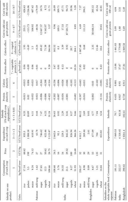
elasticities, it is possible to calculate the elasticities for two main nutrients (proteins and calories) by using the Equations 7 and 8 (Table 5).

The result shows that these Marshallian price elas-ticities for each nutrient are very low. This is due to the fact that nearly all products have nearly similar composition of proteins and calories (except sugar and oils, which contain almost no protein but are richer in calories). So when the price of one product increases by 1%, the consumption of all products modi-fies, but the total intake of protein and calories is not much modified (except for sugar and oils mainly for Pakistan). For wheat, we have more important effects on both nutrients due to the fact that when the price alone increases, it has an important negative effect on the apparent purchasing power and the whole consumption of vegetable food products, mainly in Pakistan and India. The expenditure elasticities are more important as an increase in revenue increases the consumption of all products as well as the total protein and caloric intakes. A hypothetic subsidy of 1% on prices for each product has a limited impact on the protein and caloric intakes (colons 7 and 8 of Table 5), except for wheat in Pakistan and India, as well as rice in India and mainly in Bangladesh. It is then possible to calculate the subsidy level, which is theoretically necessary to increase the protein and caloric intake by respectively 1g/head/day and 100 Kcal/head/day.

We can see (colons 9 and 10) that the most efficient way to achieve this amelioration in nutrition is, if the government chooses to subsidize wheat in Pakistan and India as well as rice in Bangladesh. This strategy can be compared on a theoretical base with a public policy to subsidize the global whole expense concern-ing the vegetable food products. In this case, there is nearly no substitution between the products and it is generally less expensive than any other policy. From these data, it would be possible to calculate for each country the total cost of subsidy to aid the most vulnerable parts of the population by assuming that they have the same initial consumption per head and the same matrix of elasticities like the average consumer, which is an important hypothesis.

DISCUSSION

The consumption of major foods has revealed a structural shift in the dietary pattern due to the changes in tastes, the easier access, the income in-crease, changes in the relative price and the urbani-zation pattern (Radhakrishna and Ravi 1992; Kumar 1998; Murthy 2000; Kumar et al. 2011; Mukherjee et al. 2011), but still cereals occupy a central posi-tion in the dietary pattern of Pakistan, India and Bangladesh (Chaterjee et al. 2007; Mukherjee et al. 2011; Zaman 2011).

According to other studies (Mittal 2006; Chaterjee et al. 2007; Kumar et al. 2011), cereals in India are expenditure inelastic products, but in our study all products are expenditure inelastic except for wheat and edible oils. Edible oils are expenditure elastic, like the peanut oil in other study (Pan et al. 2008). This implies that as the expenditure or the income level increases, the proportion of expenditure or income on wheat and edible oils is much higher than on other products in our analysis. On the other hand, all the products in our analysis are price inelastic showing that the demand of the staple food may not be affected adversely by an increase in the food price inflation (Kumar et al. 2011).

For Pakistan, all the products taken into the analysis are price inelastic like in other studies (Bouis 1992; Haq et al. 2011). According to Haq et al. (2011), wheat is a staple food in Pakistan, therefore the price increase does not change much its consumption. Expenditure elasticities indicated that all products are normal goods except for dry beans and millet/ sorghum. Rice and wheat are expenditure inelastic, which means that when the expenditure or income increases, the consumer prefers to buy other ex-pensive item.

On the contrary, in Bangladesh all the products in our analysis are expenditure inelastic except of wheat, while edible oil is an inferior good. However, according to other studies (Ali 2002; Huq and Arshad 2010), all cereals are expenditure inelastic except of wheat. The compensated own price elasticity indi-cated that all food items except for millet/sorghum are price inelastic. In Bangladesh, rice represents a major part of food as the staple product, so here the price inflation does not affect its consumption like in India.

CONCLUSION

The study delineates a model to estimate the price demand elasticity of different vegetable products and

empirically applies the model to estimate the own and cross price demand elasticity of major vegetable products that cover more than 80% of the total food consumption in Pakistan, India and Bangladesh. The data used in this study are collected from the FAO database. The Marshallian elasticities and their decomposition into the price effect and income effect, as well as the expenditure elasticities have been calculated. Then different means to increase the protein and energy intake by vegetable products are analyzed after calculating the protein and caloric elasticities.

REFERENCE

Alderman H. (1988): Estimates of consumer price response in Pakistan using market price as data. Pakistan Devel-opment Review, 27: 89–107.

Ali M., Arifullah S., Memon H.M. (2008): Edible oil deficit and its impact on food expenditure in Pakistan. The Pakistan Development Review, Pakistan Institute of Development Economics, 47: 531–546.

Ali Z. (2002): Disaggregated demand for fish in Bangla-desh: an analysis using the almost ideal demand system. Bangladesh Development Studies, 28: 1–45.

Behrman J.R., Deolalikar A.B. (1987): Will developing countries nutrition improve with income? A case study from rural South India. Journal of Political Economy, 95: 492–507.

Bouis H.E. (1992): Food demand elasticities by income group by urban and rural populations for Pakistan. The Pakistan Development Review, 31: 997–1017.

Carrasco B., Mukhopadhyay H. (2012): Food Prices Escala-tion in South Asia – A Serious and Growing Concern. South Asia Working Paper Series No.10, Asian Devel-opment Bank.

Chatterjee S., Rae A., Ray R. (2007): Food Consumption and Calorie Intake in Contemporary India. Discussion Paper No. 07.05, Massey University, Department of Ap-plied and International Economics. Available at http:// econ.massey.ac.nz/publications/discuss/dp07-05.pdf Deaton A., Muellbauer J. (1980a): An almost ideal demand

system. Economic Review, 70: 312–326.

Deaton A., Muellbauer J. (1980b): Economics and Con-sumer Behaviour. Cambridge University Press, Cam-bridge.

FAPRI elasticity database. Available at http://www.fapri. org/tools/elasticity.aspx

FAO (1966–2008): FAO Agro Statistical Database. Available at http://faostat.fao.org/site/339/default.aspx

Gomez P. (2008): Emerging Asia and International Food Inflation: The Case of Colombia. Latin America Econo-Monitor, No. 512.

Haq Z.U., Nazli N., Meilke K., Ishaq M., Khattak A., Hashmi A.H., Rehman F.U. (2011): Food demand patterns in Pakistani Punjab. Sarhad Journal of Agriculture, 27: 305–311.

Holt M.T., Goodwin B.K. (2009): The Almost Ideal and Translog Demand Systems. In: Contributions to Eco-nomic Analysis, Chapter 2, Quantif ying Consumer Preferences (ed. Slotje D.). Emerald Group Publishing Limited, pp. 37–59.

Huq A.M., Arshad F.M. (2010): Demand elasticities for different food items in Bangladesh. Journal of Applied Sciences, 10: 2369–2378.

Hussain A., Routray J. K. (2012): Status and factors of food security in Pakistan. International Journal of Develop-ment Issues, 11: 164– 85.

Kumar P. (1998): Food Demand and Supply Projections for India. Agricultural Economics Policy Paper 98-01. Indian Agricultural Research Institute, New Delhi. Kumar P., Kumar A., Parappurathu S., Raju S.S. (2011):

Estimation of demand elasticity for food commodities in India. Agricultural Economic Review, 24: 1–14. Laap S. (1990): Relative agricultural prices and monetary

policy. American Journal of Agriculture Economics, 72: 622–630.

Malthus T. (1798): An Essay on the Principal of Popula-tion. J. Johnson, London.

Mellor J.W. (1983): Food Prospects for the Developing Countries. IFPRI. Reprinted from the American Eco-nomic Review, 73: 239–243.

Mittal S. (2006): Structural Shift in Demand for Food: Projections for 2020. In: Indian Council for Research on International Economic Relations, Working Paper No. 184. Available at http://www.eldis.ids.ac.uk/vfile/ upload/1/document/0708/DOC23553.pdf

Mukherjee N., Choudhury A.G., Khan M.F.A., Islam A.S. (2011): Implication of Changing Consumption Pattern on Food Security and Water Resources in Bangladesh. In: Proceedings of the 3rd _{International Conference on}

Water and Flood Management, January 8–10, 2011, Dhaka, pp. 731–738.

Murthy K.N. (2000) : Changes in taste and demand pattern for cereals: Implication for food security in semi-arid tropical India. Agricultural Economics Research Re-view, 13: 26–53.

Pan S., Mohanty S., Welch M. (2008): India edible oil con-sumption: A censored incomplete demand approach. Journal of Agricultural and Applied Economics, 40: 821–835.

Radhakrishna R., Ravi C. (1992): Effects of growth, rela-tive price and preferences of food and nutrition. Indian Economic Review, 27: 303–323.

SOFI (1999): The State of Food Insecurity in the world. FAO Corporate Document Repository.

SOFI (2011): The State of Food Insecurity in the world. FAO Corporate Document Repository.

Trostle R. (2008): Global Agriculture Supply and Demand: Factors Contributing to the Recent Increase in Food Commodity Prices. A Report from the Economic Re-search Service. Available at http://www.ers.usda.gov/ Publications/WRS0801/WRS0801.pdf

UNCTAD price database. Available at http://www.unctad. org/templates/Page.asp?intItemID=1889&lang=1 World Bank (1981): World Development Report. World

World Bank South Asian region (2010): Food Prices In-creases in South Asia. National Responses and Regional Dimensions. World Bank, Washington.

Yaseen R.M., Dronne Y. (2011a): Estimating the supply response of main crops in developing countries: The case of Pakistan and India. ARPN Journal of Agricultural and Biological Science, 6 (10).

Yaseen R.M., Dronne Y., Ahmad I. (2011b): Estimates sup-ply response of major crops in Bangladesh. Bangladesh Development Studies, 14 (4).

Zaman U.K. (2011): Food production and consumption pattern in Pakistan during 1979 to 2010. Journal of Agricultural Biotechnology and Sustainable Develop-ment, 3: 108–119.

Received: 18th February 2014 Accepted: 20th _{May 2014}

Contact address: