FE modelling strategies of weld repair in pre stressed thin components

FE modelling strategies of weld repair in

pre-stressed thin components

Gervasio Salerno

, Chris Bennett

, Wei Sun

, and Adib Becker

1_{Gas Turbine and Transmissions Research Group, Faculty of Engineering, The}

University of Nottingham, University Park, Nottingham, NG7 2RD, UK

Abstract

Two computational procedures have been developed in the commercial finite element (FE) software codes Sysweld and Abaqus to analyse and predict the residual stress state after the repair of small weld defects in thin structural components. The numerical models allow the effects of the repair to be studied when a pre-existing residual stress field is present in the fabricated part and cannot be relieved by a thermal treatment.

In this work the modelling strategies are presented and tested by simulating a repair of longitudinal welds in thin sheets of Inconel 718 (IN718). Although the numerical strategies in the two codes are intrinsically different, the results show a significant agreement, predicting a notable effect imposed by the initial residual stress.

Keywords: Finite element modelling; Weld repair; Residual stress; Abaqus; Sysweld

1

Introduction

is carried out in an area with a pre-existing stress that may have an effect on the final residual stress distribution.

The methodology for simulating a generic fusion welding process is well es-tablished with a significant amount of works available in the literature. Based on the FE analysis, the numerical approach is a powerful and well-proven tool for predicting the macro-scale effects of both arc and beam welding processes. The applicability of the numerical predictions is also recognized in different in-dustrial fields, although here the main concern is to reduce computational costs associated with the analysis of large geometries while keeping an acceptable level of accuracy in the predictions. An excellent review of the numerical approach is from Lindgren [2]. Less attention has been focused on the simulation of weld repair, particularly on the effects of pre-existing stresses in structural compo-nents where a weld repair is needed. The main volume of research in this area is related to either aged or deteriorated materials in the nuclear, petrochemical or power industries. Thick pipes are the most common geometries analysed due to their large usage in these sectors.

et al. [10] produced numerical models for the experimental test cases studied by Bouchard and were able to get an overall agreement between measurements and prediction with a simplified block-dumped approach: the entire length of a weld pass was supposed to be deposed simultaneously, neglecting the real pro-gression in weld metal deposition. To further reduce the computational cost, they defined a FE model with a relatively coarse mesh in the area of the heat source pass, an uncommon choice for work of this kind as a fine mesh should be used here in order to better approximate the weld pool shape and simulate the steepest temperature gradients [11]. Comparisons appeared less satisfactory at mid-length and the end of the long repair. Residual stresses associated with the original girth weld were not represented in any of their FE models because they judged the predicted stresses close to the repair relatively unaffected by the prior stress field. A different geometry was examined by Jiang et al. [12,13] who considered the effects of the repair weld of a flat stainless steel clad thick plate. Simulating the repair as a multi-pass weld with material deposition and assuming a virgin state as the initial condition for the plate, they highlighted some correlations between the residual stress distribution, repair length, welding heat input and number of layers. Despite the different geometry, they found a great effect imposed by the repair length on the transverse stress distribution in agreement with findings from Dong [7]. They showed that increasing the repair length or the heat input caused the transverse stress to decrease, while a little effect was predicted on the longitudinal distribution. Also when the groove was filled with more layers, both the longitudinal and transverse residual stresses appeared to be decreased.

In the research mentioned above, the common strategy for predicting the residual stress caused by the repair procedure with FE analysis consists of treating it as a new weld: any existing residual stress due to the history of the components is assumed to be zero in the numerical models, although there is no clear evidence in the literature that the approximation can always be safely accepted, particularly when the repair is carried out immediately after a faulty joining process. To the best of the authors’ knowledge, the only work contrary to this approach is from Dong et al. [14]. While studying weld repair in the case of pipe geometries, they concluded that the pre-existing original weld stresses had a very little effect on the repair residual stress characteristics predicted from their numerical model. They highlighted that the effect might not be equiva-lent if the repair depth is different from the one they considered, or if the repair welds are located near the weld start/end positions, which they did not consider because the initial stress field was mapped from an axisymmetric simulation into the 3D model. A more recent work from Deng and Kiyoshima [15] has shown the effect of an initial special heat treatment on the final residual stress induced by a laser weld in a pipe. Although the authors did not investigate a repair but a fabrication weld, they recommended to carefully consider any other fabrication process, besides the welding, which potentially introduces residual stresses into a component, if the interest is to accurately predict the final stress state.

package Abaqus, for the prediction of residual stress in weld repair of thin struc-tural components when the procedure is applied to correct defects caused by the manufacturing phase or damage due to the operative life. While Sysweld is designed to perform welding simulations with inbuilt special functions, a gen-eral FE code requires programming of specific subroutines in order to perform numerical simulations of welding processes. The choice of using a second FE code, like Abaqus, allowed the authors to benchmark the work conducted with Sysweld. In both the numerical strategies, the pre-existing weld residual stresses are not neglected and the models provide the opportunity to investigate both the effect of the repair on the original residual stress and vice-versa. The ap-proaches are tested using the simulation of a repair of a bead-on-plate weld of an IN718 thin sheet. The details of, and associated experimental data for, the original weld (assumed to be flawed) are taken from the study of Dye et al. [16]. The experimental data have been used to validate the predictions from both the thermal and mechanical analyses performed in both of FE codes, in terms of temperature and residual stresses, for the original weld. The predicted macro-stresses from the repair modelling approach developed in each FE soft-ware are presented and compared in terms of fields and along specific paths of interest. The effects of neglecting the initial weld in the modelling of the repair process are also shown. Further applications of the models and benefits of the approaches are discussed.

2

Methodology

When a weld exhibits a localized defect, the repair process consists of removing a sufficient volume of material around it with a machining process, such as milling or partial milling, creating an excavation that is then refilled with a subsequent welding process with filler deposition. If the defect being repaired is small, only a small volume of material is removed, and the remaining part of the fabricated structure retains a residual stress state determined by the original weld. In the present work it is assumed that the potential defect has a negligible effect on the residual stress distribution caused by the initial weld. In this section the repair test case and the computational strategies are presented.

2.1

Case study

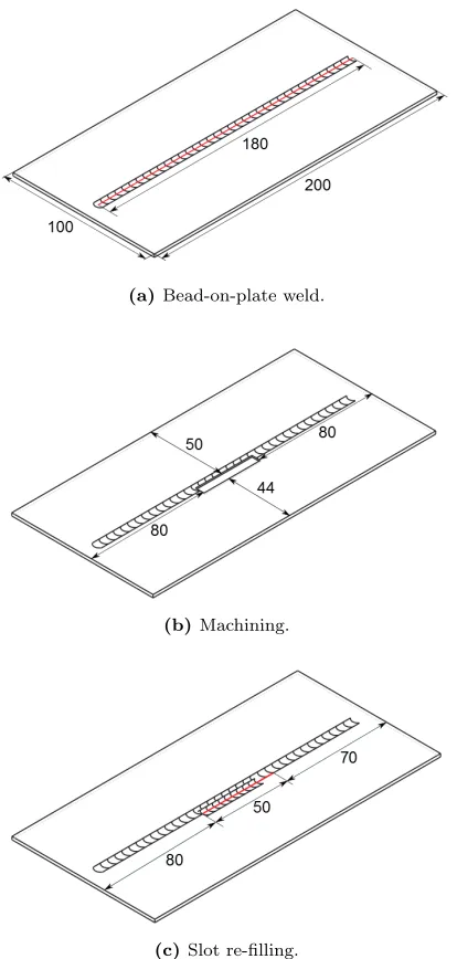
A tungsten-inert gas welding (TIG) is used to fabricate bead-on-plate in a 2 mm thick sheet. The thin plate is 200 mm long and 100 mm wide. The weld is 180 mm long, with start/end located at 10 mm from the sheet edges as shown in Fig. 1a. The process is autogenous, i.e. without filler, with the parameters shown in Table1.

Table 1: Summary of welding parameters.

Velocity 1.59 mm s−1 Peak current 80 A Base current 40 A Frequency 2 Hz Pct cycle at peak current 60 Torch-work potential 9 V

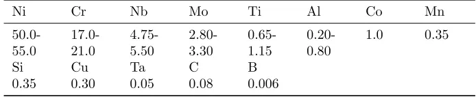
Table 2: Nominal chemical composition of IN718 (in wt%)

Ni Cr Nb Mo Ti Al Co Mn

50.0-55.0 17.0-21.0 4.75-5.50 2.80-3.30 0.65-1.15 0.20-0.80 1.0 0.35

Si Cu Ta C B

0.35 0.30 0.05 0.08 0.006

solution-heat-treated condition, the condition which the nickel-based superalloy is generally welded in.

As a small defect is assumed to exist at the boundary of the HAZ and the fusion zone, the repair procedure is defined as follows. The defective part is removed creating a rectangular slot, 40 x 6 mm, 1 mm deep across the thickness, located as shown in Fig. 1b, with one side exactly on the weld central line of the initial weld. The slot is refilled with a single TIG weld pass, with filler deposition. For convenience, the process is assumed to be equivalent to the initial weld, but the welding power is set to 680 W, chosen using the FE thermal analyses to ensure the filler material will reach the melting temperature during the deposition process. The path for the second weld starts 10 mm ahead of the slot (Fig 1c). The distance between the two weld central lines is 3 mm. The plate is unclampled during both the weld and repair process.

2.2

Theoretical background

In this section the theoretical basis of computational welding mechanics for a fusion joining process is briefly presented. As the amount of heat generated by the mechanical deformation of the material is negligible compared to the heat from the arc or beam, a sequentially coupled analysis is generally adopted. This consists of an initial thermal analysis to predict the thermal field imposed by the welding process into the fabricated structure, and solving the equation that governs the heat flow:

k

_∂2_T

∂x2

+k

_∂2_T

∂y2

+k

_∂2_T

∂z2

+G=ρC∂T

∂t (1)

(a)Bead-on-plate weld.

(b)Machining.

(c)Slot re-filling.

can be modified to take into account the latent heat of fusion/solidification and possible solid-phase transformations, but both the effects are not modelled in the present model. Coupled with initial and boundary conditions, it is solved by means of FE analysis. The predicted thermal field is then transferred as an input into the mechanical model. As the inertia effects are negligible, the process is considered quasi-static. The equilibrium equation is simply given by:

{σ}+{f}={0} (2)

where {σ} is the stress vector representing the internal force that balances {f}, vector of the external forces. The stress tensor is assumed to be symmet-rical, i.e. σij =σji. Stress-strain relations are expressed as in Eqs. 3:

{dσ}= [Dep]{dε} −[Cth]{dT} (3a)

[Dep] = [De] + [Dp] (3b)

where [De], [Dp], [Cth] are the elastic, plastic and thermal stiffness matrix, while{dσ},{dε} and{dT} are respectively the stress, strain and temperature increments. Again the problem is numerically solved by means of FE analysis.

2.3

Computational models

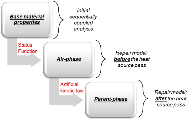
The computational models were implemented in the commercial FE codes, Abaqus and Sysweld, made up of three macro-steps as shown in Fig. 2:

The first step is a sequentially coupled thermo-mechanical analysis that im-poses the initial stress state for the subsequent repair model. The second and third steps are part of the repair modelling strategies discussed in detail in sec-tions2.7 and2.8. The element deactivation is purely mechanical and involves the computation of a new equilibrium condition to accommodate the material removal. The final step is, again, a sequentially coupled thermo-mechanical analysis that includes the simulation of filler deposition. The significance of the original weld residual stress distribution was also investigated by repeating the foregoing modelling procedure but leaving out the first sequentially coupled analysis.

Figure 2: Outline of the modelling strategy.

2.4

Mesh design

Figure 3: Cell used to make up the full meshes.

repair procedure was not symmetrical. The entire mesh contains 30560 elements and 40605 nodes and was used to solve the thermal and mechanical problems. 8-node linear heat transfer brick and 8-8-node linear brick elements were selected in both Abaqus and Sysweld for the thermal and mechanical analyses, respectively.

2.5

Material model

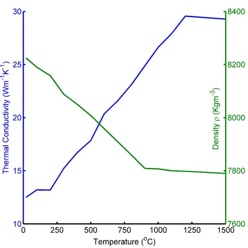
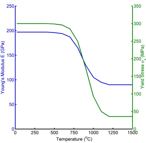
The thermal and mechanical properties for IN718 were defined as temperature dependent as in Dye et al. [16] shown in Figs. 4, 5 and 6. The Poisson’s ratio was taken to be 0.33 (temperature independent). To account for heat transfer due to fluid flow in the weld pool, the thermal conductivity was almost tripled for temperatures above the material solidus temperature (1260◦C). This assumption is not necessary using Sysweld as the software sets the selected melting value as cut-off temperature when transferring the predicted thermal field into the mechanical model. In other words, the maximum temperature perceived from the mechanical model is the chosen melting value. This was set to 1240◦C (slightly lower than the solidus temperature as in [16]). The release of latent heat during solidification was not accounted for.

Figure 4: Specific heat and thermal expansion coefficient.

Figure 5: Thermal conductivity and density.

ε=εe+εp+εth (4)

where the three components on the right hand side of Eq. 4 are the elastic, plastic and thermal strains, respectively. The elastic strain was modelled with the isotropic Hooke’s law, while yielding was defined using the von Mises crite-rion. A rate-independent model with a linear isotropic hardening behaviour was assumed for the plastic material properties. The thermal strain is computed by means of the temperature-dependent mean expansion coefficient.

The default mechanical treatment of the weld pool was selected in the two software. The annealing option in Abaqus resets the equivalent plastic strain (εpeq) when the temperature of the material point is greater than the selected

annealing value. If the temperature falls below the annealing temperature, plastic strain is accumulated again. In Sysweld the fusion option zeroes the total strain when the temperature exceeds the selected value.

2.6

Thermal and mechanical boundary conditions

Figure 6: Young’s modulus and yield stress.

were both included as heat loss mechanisms with Newton and Stefan-Boltzmann laws, respectively. The second effect dominates at higher temperatures near and in the weld zone, while the first effect is more relevant for lower temperatures away from the weld zone. The convective and emissivity coefficients were set to 25 W/m2 _{and 0.8 respectively [17].}

Several heat source models may be found in the literature to catch the weld pool shape and properly simulate the weld heating for different fusion welding processes. The double ellipsoid developed by Goldak et al. [11] is a common choice for TIG. However as thickness of the sheet is small in this case, a 2D Gaussian distribution of the heat power gives a good approximation of the heating process and is also preferred due to the reduced number of parameters to be selected. The powerQis distributed as:

Q=Q0e  −

(x)2_{+ (y−v·t)}2

r2 0

 

(5)

wherev,t,r0 andQ0 are the welding velocity, integration time step,

velocity) [18]. While the welding power was set to 560 and 680 W for the weld and repair thermal analyses, r0 and η were respectively set to 4 mm and 0.7

with a trial/error approach to ensure that the thermal predictions for the ini-tial weld were in good agreement with the experimental observations, using a combination of two approaches: thermal histories and weld pool shape compar-ison between predictions and experimental tests. Same values forr0andη were

maintained for the repair weld as well.

It is worth highlighting that the dimension of Q in Eq. 5 depends on the FE code used, as Sysweld requires a power (W) [19], while Abaqus expects a power density, W/[L2_{] when the heat is applied onto a surface, as in this case,}

and W/[L3_{] if the heat is applied in a volume [20]. As large differences in the}

thermal predictions are reflected in the mechanical results, a check on the heat flux (W/[L2_{]), both in the magnitude and the distribution, was used to ensure}

that the heat given in input in the two FE codes was consistent.

Figure 7: Location of the nodes for the mechanical constraints.

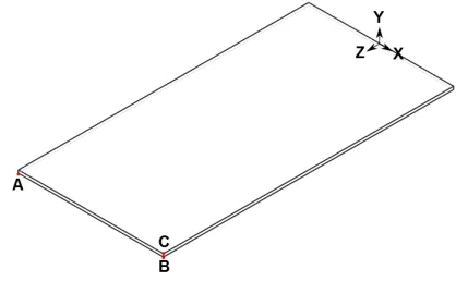
Constraints were applied in the mechanical analyses only to prevent rigid body motions as the sheet was free to deform during the whole process. An artificial boundary condition was imposed as follows (Fig. 7):

• node A constrained along X,Y,Z

• node B constrained along Y,Z

• node C constrained along Z

2.7

Repair modelling in Abaqus

the model. These are gradually ramped down to zero during the removal step, to ensure the new equilibrium condition is smoothly recomputed in the rest of the model, and the solution converges. Elements remain inactive in subsequent steps unless the user changes their status. Internal forces associated with them are removed from the results because they are not considered in the computa-tion process by the software, starting from the beginning of the step in which they are deactivated. This is advantageous from a computational point of view, particularly when the area deactivated is relatively large (many elements), but it can also cause issues when elements need to be reactivated in the subsequent phase. The deactivation effect imposes a new equilibrium condition, causing both a redistribution and potentially a release in the residual stress field, de-pendent on the extent and the location of the part deactivated. Although the residual stress in proximity of the deactivated area may not be a good represen-tation of the actual one caused by the physical removal process, the simplified numerical strategy can still be adopted, based on the assumption that the effect on the local residual stress field is dominated by the subsequent refilling welding process. A new sequentially coupled analysis was then carried out to simulate the effects of the slot refilling. Dead elements in the slot were reactivated (model change → add) in a “reset” status (i.e. zero stress, strain & plastic strain) in order to simulate the filler deposition. If all of them were reactivated at the same time, they would have the material properties assigned as in the initial weld simulation. When the heat source approaches them, the part of material in front of it would react both in the thermal and mechanical analyses, although it is not physical existent yet. However, when the heat source moves along the welding path, the material in front of it has less influence on the thermal field than the one behind it, because the heat flow in the welding direction is slower than the weld speed. Therefore, the material deposition can be ignored in the thermal analysis [22]. Also, from the authors’ experience, the reactivation pro-cedure in the thermal analysis causes instabilities in the predicted temperature histories because the code imposes a ramping for the material thermal conduc-tivity from a zero value to the actual one. Unless elements are made thermally active slightly ahead of the torch, the simulated weld pool will not be stable, showing sudden drops and increases in temperature. As there are no relevant differences in the predicted thermal fields using this approach or avoiding the elements deactivation/reactivation, it is recommended to ignore the actual ma-terial deposition in the thermal analysis, significantly saving time in the model preparation.

A sequential reactivation of elements in the slot, grouped into pre-defined sets, was coded in the mechanical step in order to simulate the deposition effect. Fig. 8shows the reactivation of a set in terms of the von Mises stress and weld pool position in the corresponding thermal frame. A new analysis step was created for each set being reactivated, making the model preparation repetitive and prone to mistakes. Hence a python script was used to automate the step definition process in Abaqus.

Figure 8: Filler deposition procedure in Abaqus.

predicted thermal history: this ensures that the stress-free elements will give the appropriate mechanical contribution in the model as soon as their temperature falls below the annealing value, 1240◦C in this case. Since the software does not perform any calculation for deactivated elements, the strategy is equivalent to the so-called “inactive element” approach described by Lindgren and Hedblom [23], one of the two possible procedures used in the literature to simulate ma-terial deposition in FE analysis. The main issue was already discussed in the mentioned work: nodes of the removed elements remain at the location occupied at the time of deactivation, causing their new configuration (when reactivated) to be significantly different from the one specified when defining the initial FE model, particularly in large-displacement analysis. This could negatively affect the quality of the results or totally prevent convergence of the solution. The easiest way to bypass the problem was found in defining a duplicate set of ele-ments on top of the removed ones, whose material properties did not influence the solution [20]. These duplicate elements only provide a means of updating the position of the nodes of the removed elements when they are deactivated.

2.8

Repair modelling in Sysweld

equivalent to the so-called “quiet element” approach described by Lindgren and Hedblom [23] as an alternative numerical strategy to simulate material depo-sition in FE analysis where, the not yet deposited filler is considered in the computation process. Although zeroed out of the load vector, stress associated with deactivated elements still appears in element-load lists.

As the deposition effect in the thermal analysis showed analogous issues as described in the previous section (unstable temperature in the weld pool with non-physical drops and increases), it was also neglected in the Sysweld analysis. In this case the software only applies the reduction factor on the mechanical material properties. After the original residual stress was introduced into the model by means of the initial sequentially coupled analysis, the status function for elements in the slot was shifted from 1 to -1, which imposes a new equilibrium condition that accommodates the stiffness reduction of deactivated elements. The same problem, as discussed in the previous section, had to be considered: elements in the slot cannot be reactivated, all at the same time, by simply re-shifting the status function value. This is because, elements in front of the torch would give a mechanical contribution when that area is not physically existent yet.

Figure 9: Evolution of material properties for elements in the slot.

phase defined with the mechanical properties shown in section2.5. The diagram in Fig.9shows the evolution of material properties for elements in the slot based on the current analysis step.

Figure 10: Filler deposition procedure in Sysweld.

Fig. 10 shows the elements reactivated as air-phase, representing the not yet deposited filler, and their conversion into parent-phase while the heat source approaches and passes on them. In the mechanical analysis this ensured that the material being deposited was numerically treated as air when ahead of the torch, soft-solid when the torch was on it, and solid after the torch pass.

3

Results

3.1

Results of thermal analyses

experi-ment and FE predictions from the models in the two software codes. The small difference in temperatures between the two software codes (30◦C maximum) causes the weld pool predicted in Abaqus to appear slightly wider than the one in Sysweld, but the shapes are equivalent. It is evident from the experimen-tal macrograph that the welding process caused the material to entirely melt through the thickness. The numerical heat source selected for the modelling was suitable to predict this effect. For the sake of completeness, in Fig. 13 the predicted thermal histories are shown in the case of the repair weld at a distance of 6, 8 and 10 mm from the weld path on the sheet top surface. Again a very good agreement is visible in the numerical results, confirming that the two software codes compute very similar thermal fields when consistent heat powers are assigned as an input. As expected, maximum temperatures at each location are higher than the corresponding ones from the previous analysis, as the effective weld power was increased to ensure the filler melted.

Figure 12: Real [16] and predicted weld pool shape from the FE codes.

3.2

Results of mechanical analyses

Figs. 14and15show the evolution of the strains and thermal histories in a node from the weld pool, with the aim of presenting the different treatment of the weld fusion zone imposed by the FE codes. For clarity, only the strain component in the weld direction is shown. The cut-off effect imposed by Sysweld in the temperature history, when transferred into the mechanical model, is noticeable in the constant value of 1240◦C between 55 and 60 s (when the node is in the weld pool). Conversely, the temperature that Abaqus transfers into the mechanical model reaches a peak in the same time frame. When the temperature reaches the melting value, Sysweld zeroes all the strain components, whatever the value is immediately before. In Abaqus, althoughεp

eq is the only strain component

zeroed, the effect is still visible on the total strain as a sudden drop. However, the plastic strain is not totally reset, causing bothεp _{and consequentlyεto be}

similar in trend but significantly different in magnitude when the node cools down. Disregarding the zeroing in the highlighted time frame, both the elastic and thermal strain histories present comparable trends.

Four paths were selected to compare the residual stress: paths 1 and 3 are located at the start and end of the repair slot as shown in Fig. 16, path 2 is located in the middle of the repair and path 2’ (not visible in Fig.) is parallel to path 2 but located at half thickness where residual stress measurements were taken. Longitudinal and transverse stresses are compared with neutron diffraction measurements along path 2’ in Figs. 17 and 18after the bead-on-plate weld. The experimental measurements show trends and magnitudes which are well correlated with the numerical results. The longitudinal stress presents a typical distribution for welded structures, with a tensile area close to the weld path that becomes compressive moving towards the sheet edges. Less correlation is found in the compressive region, while this occurs close to the weld path area for transverse stress distribution.

Figure 13: Repairing weld: measured and predicted thermal cycles at 6, 8 and 10 mm from the weld center line at approximately the mid-length of the weld.

codes are in good agreement, with the highest and lowest peaks at the same lo-cations. The region surrounding the refilled slot shows the highest longitudinal tensile stress, with the highest peaks occurring in the area that corresponds to the initial weld. As for the initial weld, the peaks are due to the annealing effect in Abaqus (fusion temperature option in Sysweld), occurring where the temper-ature reaches 1240◦_{C. In proximity of the slot refilled, the longitudinal residual}

stress appears relatively less invariant in the weld direction than the transverse stress. This, conversely, shows a complex and highly variable distribution. In both cases the distributions are totally tensile along the paths considered. Also the longitudinal stress is still more important than the transverse stress, in terms of magnitude.

Figure 14: Thermal and strains histories in a point in the weld pool. Abaqus (solid line) Sysweld (dashed line).

predictions from the two FE codes, the comparison shows an underestimation in the maximum longitudinal residual stress when the pre-existing stress field is neglected. The peak occurring in the HAZ of the initial weld is approximately 100 MPa lower both in the Abaqus and Sysweld results. The distributions are both tensile close to the refilled slot, but the disparity tends to be marked, moving to the sheet edges where signs of the stress become opposite, i.e. com-pressive when the initial stress is neglected, tensile when it is not. Although the distribution after the repair in Fig. 21may suggest there is not equilibrium along path 2, the cross section in Fig. 22shows that the longitudinal stress is self-equilibrated, both after the initial and repair weld, highlighting tensile and compressive areas.

Figure 15: Thermal and strains histories in a point in the weld pool. Abaqus (solid line) Sysweld (dashed line).

tensile transverse stress appears slightly different, particularly after the repair and neglecting the original stress. Despite some disparities, the characteristic transition from tensile into compressive at the start/end weld is still clear and predicted from both Abaqus and Sysweld. Finally, a significant redistribution of the initial stress is notable from the presented results. Also, both the pre-dicted stress distributions appear significantly different when the original stress is neglected.

4

Discussion

ef-Figure 16: Location of reference paths.

fect of the different mechanical treatments of the weld fusion zone, as Sysweld zeroes the total strain when the temperature exceeds the selected melting value, while Abaqus only zeroes the equivalent plastic strain.

Numerical results from the two codes show a very good correlation both in terms of thermal histories and the weld pool shape, with Abaqus predicting a slightly higher temperature than Sysweld, in agreement with findings from Deshpande et al. [17]. A possible explanation for the different predicted and measured cooling rates can be found in the heat loss mechanisms. These were numerically imposed on all the sheet surfaces, while in the experimental test, the plate was partially insulated from the jig using a graphite backing plate. Therefore, the model predicts a faster cooling rate than the real case, and also causes the predicted fusion zone to have a slightly different shape from the real one. This possibly affects the mechanical results as well, producing some visible incongruities when compared to the neutron diffraction measurements. The simulation of the partial heat loss due to the conduction between the IN718 sheet and the graphite backing plate could improve the agreement between predictions and experimental results. However, as the main aim of the work was to present the weld repair modelling strategies, the predicted stress fields for the original weld were judged to be sufficiently accurate to be uses as initial conditions in the FE models.

The repair modelling strategies, summarized in Table 3, predict very com-parable distributions for the longitudinal and transverse stress. The differences are believed to be mainly due to a combination of three distinct effects:

• small differences in the initial stress;

• treatments of the weld pool imposed by the two software codes;

• intrinsic differences in the implementation of the weld repair models.

Figure 17: Longitudinal residual stress after initial weld along path 2’.

limit the maximum temperature and only resets the equivalent plastic strain, leaving the other components unaffected. The third point mainly concerns the procedure adopted to simulate the material deposition. In the groove filling step, Abaqus does not consider the not yet deposited filler in the mechanical computation process when it is not physically existent, while Sysweld does, con-sidering those elements with a reduced stiffness. In the case of Abaqus, elements simulating the filler do not give any mechanical contribution in the model till they are deposited (becoming mechanically active again). In the case of Sysweld they give a mechanical contribution and exert an effect on the surrounding ma-terial even when they are not physically existent yet. This certainly causes the strain and, consequently, stress histories to have a different evolution in the two FE models during the heating phase of the groove refilling step, that is clearly reflected in the final state when the sheet cools down.

per-Figure 18: Transverse residual stress after initial weld along path 2’.

fectly agree with the findings by Dong et al. [7,24] i.e. the increased magnitude compared to the initial one and the sharp fall from tensile into compression beyond the ends of the repair. Also the relative uniformity of the longitudinal stress along the repair weld direction, with highly tensile peaks near the refilled slot caused by the strong restraint imposed by the surrounding material were also discussed in the same works.

Figure 19: Longitudinal residual stress after repair procedure. Abaqus (solid line) Sysweld (dashed line).

certain distance from the fabrication weld, in the present work, the original weld stress appears to have an effect both on the repaired and, more evidently, the non-repaired area.

Figure 20: Transverse residual stress after repair procedure. Abaqus (solid line) Sysweld (dashed line).

could be also applied to predict the effect of standardised repair procedures and, potentially, to improve them in order to determine a lowered final residual stress state, by analysing the effect of different weld parameters. This perfectly adheres to the emerging idea of green welds, that promotes the avoidance of heat treatments. Also the models can certainly be a valid tool to investigate the assumption of neglecting the history, and therefore the stress field present in the component before repair, still obtaining conservative predictions.

5

Conclusions

Figure 21: Effect of the initial residual stress on the longitudinal stress. Abaqus (solid line) Sysweld (dashed line).

the numerical models. Despite the differences in the way the two software codes model some aspects of the process, predictions are in good agree-ment. A good correlation is also found with the available experimental data, both in terms of thermal histories and residual stresses, confirming that both the FE software codes can be used to predict useful data for the analysis of fatigue life and structural integrity of fabricated thin welded components.

appli-Figure 22: Longitudinal residual stress before and after repair procedure. Cross section at path 2 (Abaqus).

Table 3: Overview of the weld repair FE models in Abaqus and Sysweld.

Physical step Abaqus Sysweld

Machining model change - remove status function -1 Slot refilling model change - add

synchronized with heat source pass

status function 1 combined with artificial kinetic law

cability of the models includes all the possible cases of weld repair, where an important residual stress is already present in the component and its effect on the final stress distribution is not predictable.

• The predictions in terms of residual stress for the repair case study are relatively well-correlated, despite the methodologies using different nu-merical approaches to simulate the physical sequence of the process. The models show a significant redistribution of the initial stress caused by the repair procedure, clearly visible in the presented stress fields. Noticeable features in the numerical results are consistent with findings from previous work in the field of weld repair.

• The numerical models predict different residual stress distributions whether the pre-existing stress is neglected or not. In detail, the simulation of the repair as a new weld, i.e. neglecting the pre-existing stress, appears not to be conservative for the longitudinal tensile stress. However, it should be pointed out that the present results are based on the case study analysed.

(a)After bead-on-plate weld.

(b)After repair procedure.

(c)Neglecting the initial residual stress.

Figure 23: Longitudinal Residual Stress from Abaqus (left) and Sysweld (right).

be carefully considered, if the interest is to predict a realistic final stress state.

Acknowledgements

(a)After bead-on-plate weld.

(b)After repair procedure.

(c)Neglecting the initial residual stress.

Figure 24: Transverse Residual Stress from Abaqus (left) and Sysweld (right).

Funding

The authors wish to thank Rolls-Royce plc for their financial support of the research.

References

[1] Ram, GD Janaki and Reddy, A Venugopal and Rao, K Prasad and

[2] Lindgren, LE. Numerical modelling of welding. Computer methods in applied mechanics and engineering 2006; 195(48): 6710–6736.

[3] Brickstad, B and Josefson, BL. A parametric study of residual stresses in multi-pass butt-welded stainless steel pipes. International Journal of Pressure Vessels and Piping 1998; 75(1): 11–25.

[4] Deng, D and Murakawa, H. Prediction of welding residual stress in multi-pass butt-welded modified 9cr–1mo steel pipe considering phase transformation effects. Computational Materials Science2006; 37(3): 209– 219.

[5] Yaghi, AH and Hyde, TH and Becker, AA and Sun, W and

Hil-son, G and Simandjuntak, S and Flewitt, PEJ and Pavier, MJ and Smith, DJ. A comparison between measured and modeled resid-ual stresses in a circumferentially butt-welded p91 steel pipe. Journal of Pressure Vessel Technology 2010; 132(1): 011206.

[6] Feng, Z and Wang, XL and Spooner, S and Goodwin, GM and

Maziasz, PJ and Hubbard, CR and Zacharia, T. A finite element

model for residual stress in repair welds. Technical report, Oak Ridge National Lab., TN (United States), 1996.

[7] Dong, P and Hong, JK and Bouchard, PJ. Analysis of residual

stresses at weld repairs.International journal of pressure vessels and piping 2005; 82(4): 258–269.

[8] Brown, TB and Dauda, TA and Truman, CE and Smith, DJ

and Memhard, D and Pfeiffer, W. Predictions and measurements of residual stress in repair welds in plates. International journal of pressure vessels and piping 2006; 83(11): 809–818.

[9] Bouchard, PJ and George, D and Santisteban, JR and Bruno,

G and Dutta, M and Edwards, L and Kingston, E and Smith, DJ. Measurement of the residual stresses in a stainless steel pipe girth weld containing long and short repairs. International Journal of Pressure Vessels and Piping 2005; 82(4): 299–310.

[10] Elcoate, CD and Dennis, RJ and Bouchard, PJ and Smith, MC.

Three dimensional multi-pass repair weld simulations.International journal of pressure vessels and piping 2005; 82(4): 244–257.

[11] Goldak, JA and Chakravarti, A and Bibby, M. A new finite element model for welding heat sources. Metallurgical transactions B 1984; 15(2): 299–305.

[12] Jiang, WC and Wang, BY and Gong, JM and Tu, ST. Finite

[13] Jiang, W and Xu, XP and Gong, JM and Tu, ST. Influence of repair length on residual stress in the repair weld of a clad plate. Nuclear Engineering and Design 2012; 246: 211–219.

[14] Dong, P and Bouchard, PJ and Zhang, J. Effects of repair weld length on residual stress distribution. Journal of pressure vessel technology 2002; 124(1): 74–80.

[15] Deng, D and Kiyoshima, S. Numerical simulation of residual stresses induced by laser beam welding in a sus316 stainless steel pipe with con-sidering initial residual stress influences. Nuclear Engineering and Design 2010; 240(4): 688–696.

[16] Dye, D and Hunziker, O and Roberts, SM and Reed, RC. Modeling of the mechanical effects induced by the tungsten inert-gas welding of the in718 superalloy. Metallurgical and Materials Transactions A2001; 32(7): 1713–1725.

[17] Deshpande, AA and Tanner, DWJ and Sun, W and Hyde, TH

and McCartney, G. Combined butt joint welding and post weld heat treatment simulation using sysweld and abaqus. Proceedings of the Insti-tution of Mechanical Engineers, Part L: Journal of Materials Design and Applications 2011; 225(1): 1–10.

[18] Stenbacka, N and Choquet, I and Hurtig, K. Review of arc efficiency values for gas tungsten arc welding. In IIW Commission IV-XII-SG212, Intermediate Meeting, BAM, Berlin, Germany, 18-20 April, 2012. pp. 1– 21.

[19] SYSWELD Reference Manual. ESI Group, France 2014; .

[20] ABAQUS Analysis User’s Manual Version 6.13. Dassault Syst`emes Simulia Corp, USA 2013; .

[21] Teng, TL and Chang, PH and Tseng, WC. Effect of welding sequences on residual stresses. Computers & structures 2003; 81(5): 273–286.

[22] Lundb¨ack, A and Lindgren, LE. Modelling of metal deposition. Finite Elements in Analysis and Design 2011; 47(10): 1169–1177.

[23] Lindgren, LE and Hedblom, E. Modelling of addition of filler material in large deformation analysis of multipass welding. Communications in Numerical Methods in Engineering 2001; 17(9): 647–657.