A novel spatiotemporal home heating controller design: system emulation and field testing

Contents lists available atScienceDirect

Building and Environment

journal homepage:www.elsevier.com/locate/buildenv

A novel spatiotemporal home heating controller design: System emulation

and

fi

eld testing

Martin Kruusimägi

, Sarah Sharples

, Darren Robinson

a_{University of Nottingham, United Kingdom} b_{University of Sheffield, United Kingdom}

A R T I C L E I N F O

Keywords: Spatiotemporal heating Control algorithm Thermal comfort User experience Home automation

A B S T R A C T

We have developed a spatiotemporal heating control algorithm for use in homes. This system utilises a com-bination of relatively low-tech hardware interfaced with electric heating systems and a smartphone interface to this hardware, and a central server that progressively learns users' room-specific presence profiles and thermal preferences. This paper describes the associated spatiotemporal heating control algorithm, its evaluation uti-lising the dynamic building performance simulation software EnergyPlus, and a longitudinal deployment of the algorithm controlling a quasi-autonomous spatiotemporal home heating system in three domestic homes. In this we focus on the prediction of occupants' presence and preferred set-point temperature as well as on the cal-culation of optimum start time and the utilisation of user-scheduled absences; this for two comfort strategies: to maximise comfort and to minimise discomfort. The former aims to deliver conditions equating to a‘neutral’ thermal sensation, whereas the latter targets a‘slightly cool’sensation with corresponding heating energy savings. Simulation results confirmed that the algorithm functions as intended and that it is capable of reducing energy demand by a factor of seven compared with EnergyStar recommended settings for programmable ther-mostats. Field study results align with thesefindings and highlight the possibility to reduce energy under the minimise discomfort strategy without compromising on occupants' thermal comfort.

1. Introduction

This research is motivated by the IPCC's recommendation to achieve a 40–70% reduction in anthropogenic greenhouse gas emissions by 2050 and to fully decarbonise anthropogenic activities by 2100, to maintain global warming below 2 °C over the course of the 21st century [24]. With the Climate Change Act [29] the UK government has es-tablished legally binding targets to lower the UK's carbon dioxide emissions to 20% with respect to 1990 levels by 2050. In 2015, the domestic sector was the second-largest emitting sector (27%) in the UK, after transportation (38%) [3], with space heating contributing two-thirds of total domestic usage [26]. The UK housing stock is relatively poorly insulated and ageing, with between 85% and 97% of dwellings that will be in use in 2050 already having been built in 2006 [14]. But the expense of renovating an outdated housing stock suggests that more efficient ways of heating buildings need also to be examined. To this end, we develop and evaluate in this paper a new spatiotemporal heating control solution, which reduces the amount of energy used for heating whilst achieving occupant comfort aspirations.

Related prior studies on automated home heating control algorithms

applied a neural network to predict occupancy probability that best matched observation using data from the past few hours, the previous three days, and for same weekday over the past four weeks, suggesting possible cost savings [22]. Others used GPS positioning data from oc-cupants' phones as a trigger for a set-back mode and their simulations demonstrated that savings up to 7% could be obtained by integrating drive-home time as a trigger for re-heating the house to user-selected settings [11]. Subsequent work highlighted that a probabilistic presence schedule derived from GPS data outperformed user-reported presence schedules and driving home duration alone [17], indicating that an automated system could deliver better results for limiting heater switch-on time than a human-programmed thermostat. However, none of these studies applied these schedules to a simulated or situated heating system, thus not reflecting the complexities of managing a thermal environment to match users' expectations; nor did they adapt set-points according to users' preferences or exercise spatial dis-crimination in their control.

In afirst response to this shortfall, Gao and Whitehouse [7] de-monstrated, utilising a control algorithm that acted reactively after presence was detected, rather than proactively predicting presence and

https://doi.org/10.1016/j.buildenv.2018.02.027

Received 1 October 2017; Received in revised form 20 February 2018; Accepted 21 February 2018

∗_{Corresponding author.}

E-mail address:[email protected](M. Kruusimägi).

Building and Environment 135 (2018) 10–30

Available online 23 February 2018

catering for future occupancy, that occupants' ability to forgive the algorithm's delays in this“miss time”could be utilised to reduce heating and cooling durations, resulting in potential heating and cooling de-mands up to 15% lower than those achieved using the US recommended EnergyStar setback schedule (8 a.m.–6 p.m.). This model applied a user-selected set-point temperature based on their presence. While an in-teresting approach, the energy saving was achieved at the cost of oc-cupants' comfort, a trade-offthat would not be acceptable to all users. Another control algorithm used motion sensor and magnetic door sensor data to (1) monitor occupants' presence to switch the HVAC system offduring night-time and absences, (2) utilised previous pre-sence data to predict prepre-sence and choose between a proactive and reactive approach to heating, and (3) utilised a‘deep setback’in which the temperature was allowed to decay to 10 °C or grow to 40 °C, (further change was limited to prevent damage to the building) [20]. A static set-point of 70 °F (21 °C) was used and the authors concluded that an energy use reduction of up to 28% was possible, highlighting that deeper set-backs (allowing temperature to decay or grow more) have a larger impact on energy saving than longer (limited decay or growth allowed for a longer period) setbacks [20]. Others have included weather and building characteristics in a controller utilising a combi-nation of a proactive and reactive heating strategy, demonstrating that occupancy prediction can reduce energy spent by 9% [15]. A different approach utilised occupant discomfort history and occupancy predic-tion to constrain the expected discomfort to deliver energy savings in an office setting [21]. Whilst interesting, it would perhaps be more sui-table to understand the occupants' experience of discomfort and avoid it, rather than exploit it.

A more comprehensive approach by Scott et al. [28] gave their al-gorithm control over a gas-fired heating system in 5 households in the UK (2) and the US (3). One of thefive participating households tested a spatiotemporal control algorithm, whilst the remaining four were controlled to provide a uniform thermal environment throughout the house; both responding to predicted occupancy. User presence was detected using RFID tags and the algorithm's performance was mea-sured against a 7-day programmable thermostat schedule. Their algo-rithm pre-heated living spaces in expectation of future presence, ap-plying a user-defined set-point when the space was occupied during the day and a sleep set-point during the night. When the space was un-occupied their algorithm predicted the next un-occupied period by re-presenting space occupancy as a binary vector for each day, where each element represented occupancy in a 15- minute interval. A partial oc-cupancy vector from midnight up to the current time was used to predict future occupancy by finding similar days from the past. The algorithm then computed the Hamming distance, which simply counts the corresponding number of unequal binary vector elements between the current partial day and the corresponding parts of all the past oc-cupancy vectors, picked the 5 nearest past days and predicted presence as a mean of thosefive days [28]. Results from deployment demon-strated an 18% decrease in gas usage for individual room control and an 8% reduction for a uniform solution, showing that a spatiotemporal heating solution delivers greater energy savings. Koehler et al. [16] used a GPS-enabled smartphone application to provide location data to predict occupancy and give the smartphone control over one of ten domestic heating systems. Their algorithm used time periods of Un-necessary Heating (percentage of daytime periods when the user was away from home, but the temperature was above 15.5 °C) and Lost Comfort(percentage of daytime periods at home when the temperature was below the user's preferred temperature) periods to optimise heating times to occupant presence. The authors concluded that 44 min of un-necessary heating per day can be avoided and that their prediction model was up 6.3% more accurate than manual control, or Scott et al.’s controller [28]. While these proposed algorithms are a step in the right direction, they fail to close the thermal comfort feedback loop and dynamically account for users' thermal preferences. By that, we mean that they merely applied a user-defined set-point temperature and did

not treat this set-point as a variable that can be part of a thermal comfort dialogue.

Jazizadeh et al. used fuzzy logic to compute weighted thermal preference profiles of multi-occupant spaces using occupants' thermal preference votes, to determine dynamic heating set-points [13]. The authors gave their algorithm control over a 2-zone office space and concluded that increased comfort was delivered. It has also been de-monstrated that temperature set-point variations of ± 3 °C can lead to 7–37% savings in energy usage, depending on climate and building size [9], suggesting that additional energy savings are possible then in-cluding thermostat set-point in the control algorithm.

From this review of the key advances in advanced home heating control systems, we conclude that significant effort has been invested in strategies to predict occupancy, using a variety of data sources, to best match pre-heating and heating output with presence. Those studies that have incorporated real-life deployment have treated the thermal com-fort feedback loop as closed, so that preferred heating set-point was not included as a control variable; and few of these have addressed the domestic setting. The work presented here aims to fill this gap. We propose that including thermal sensation feedback from users over time can lower the temperature set-point; and/or better match users' spa-tiotemporal thermal preferences. Furthermore, we suggest that by nudging this set-point towards the lower end of thermal neutrality, further energy savings could be realised.

We refer the interested reader to Kruusimägi (2017) for a more detailed review of advances in home heating control systems and of joint-cognitive systems approaches [12] to include human subjects in their design and subsequent deployment, with the aim of maximising the dual objectives of acceptance and performance gains.

1.1. Aims and objectives

The aim of this paper is to develop a heating control system that delivers thermal comfort and energy efficiency and to evaluate itsfi t-ness for purpose in real-life contexts. In this we consider thermal comfort to mean that the occupant experiences a sensation of (close to) thermal neutrality in the space they occupy, and energy efficiency to mean the delivery of these conditions at minimal energy usage. For a heating control system to achieve these objectives it needs to: (i) ac-count for individual differences in occupants' thermal sensation, (ii) demonstrate an ability to adjust itself to its context, (iii) operate in relative autonomy to limit energy use in heating unoccupied spaces, and (iv) facilitate an appropriate degree of manual over-ride for occu-pants. The control algorithm of such a system would, therefore, need to: (a) capture and predict occupants' presence in the space, (b) include occupants' thermal feedback and adaptation in a heating set-point cal-culation, and (c) optimise heating system start time, to reflect the (potentially varying) thermodynamic characteristics of the space within which it operates, and (d) enable occupants to override the heating system operation and associated set-point. In addition, such an algo-rithm could be enhanced by a nudging mechanism (a variant of (b)), utilising occupants' thermal feedback to adjust the heating set-point to the lower boundary of their comfort range, thus limiting the amount of energy required without compromising on comfort.

Our interpretation of an algorithm and its underpinning technology that meets these criteria is presented in the following section. We then evaluate thefitness for purpose of the core elements of this algorithm, emulating its operation in a simulation environment, before deploying the combined system in thefield - giving the algorithm control over heating regimes in three homes for a six month period. In this way, we were able to explore the user experiences of living with such a system in a highly ecologically valid1_{setting over extended periods.}

1_{By ecological validity it is meant that a phenomenon observed in a hypothetical}

1.2. Algorithm

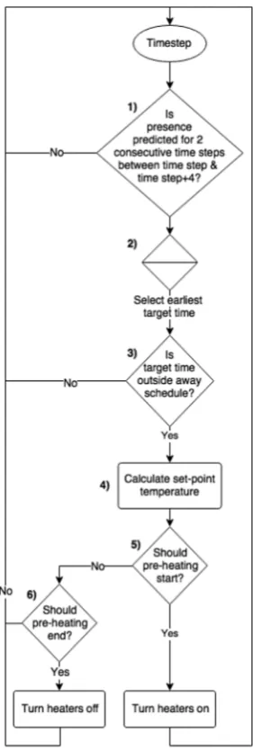
Our proposed spatiotemporal heating control algorithmfirst pre-dicts future presence probabilities (steps 1–3 inFig. 1) based on past presences for that weekday (addressing item (a) above). Predicted presences are thereafter associated with a temperature set-point (step 4 inFig. 1) based on occupants' thermal sensation feedback relating to previous set-points (addressing item (b) above). We present two var-iations of the algorithm, differing in the manner in which the set-point calculation is performed. A ‘maximise comfort’ strategy calculates a temperature at which the occupant was predicted to experience thermal neutrality on the ASHRAE 7-point scale [1], while the‘minimise dis-comfort’strategy opted for the‘slightly cool’sensation. We consider the latter to be the lower boundary of the occupant's thermal comfort range that would not cause discomfort. With future presences and set-points determined, the algorithm proceeds to pre-heat the room (steps 5&6 in Fig. 1) in readiness for the next presence (addressing item (c) above). This step utilises an optimum start algorithm that initiates activation of the heaters so that the target set-point temperature is reached at or near to the predicted start of presence. The optimum start algorithm con-tinually updates itself to reflect the physical characteristics of the space it occupies as well as other factors such as seasonality. In addition, the algorithm accounts for occupant-dependant departure schedules, re-ferring to extended, abnormal periods away from home such as holi-days or other absences, and supports the occupant in overriding pre-dicted set-point temperatures (establishing quality (d) in algorithm operation); after which the algorithm resumes normal operation.

The algorithmicflow is summarised (Fig. 1), followed by a more detailed explanation of each key feature.

At step 1) inFig. 1the algorithm calculates presence probabilities for the current and four subsequent 10-min time-steps. This calculation (1) is performed using an exponentially weighted running mean [5], which uses inputs from previous calculations for that weekday and the measured presence from the last occurrence of that weekday. Weekday differentiation was utilised to accommodate common changes in peo-ples' activities between weekdays and weekends, as well as between individual days within these work pattern-orientated categorisations. Fig. 1.Depicting the functionalflow of the proposed control algorithm.

Fig. 2.Illustrating the system design offield study technology.

Fig. 3.Illustrating the operational interactions between the server, Raspberry Pi and phone app.

= − + − − Pi (WPi21 (1 W PM) i21)

1

2 ₍₁₎

The presence probability Pfor current day i is calculated using previous predictions, measured presence PM, and a weightW of 0.8 (this relatively high value causes the algorithm to favour historic over recent data, preventing it from over-reacting to erratic user behaviour). By using previously calculated predictions in this way, we avoid the need to store the entire series (or some subset thereof), therefore lim-iting the number of data lookups and calculations that the algorithm has to perform in comparison with other exponentially weighted run-ning mean expressions, and only requires 1 week of trairun-ning data to function. The algorithm performs this calculation for the current time step as well as four time steps into the future, aiming to identify ‘meaningful presences’; defined as two consecutive time steps where P≥0.4, to represent a threshold between predicted presence and ab-sence, with predicted presence probabilities below this value being treated as predicted absences. The value of 0.4 was established during a

calibration exercise. Our four consecutive time steps, representing a 40min duration, eliminates presences where the user was likely to be present, but for a period not deemed long enough to warrant heating. Weighting the use of previous predictions and measured presence al-lows the algorithm to stay up to date with the latest changes in beha-viour, without being overly influenced by erratic and non-repeating behaviour, or indeed by outdated historic data. Consider two cases that require the algorithm to learn new behaviours–firstly, an occupant's work hours change to part-time, causing increased presence, but not to be confused with an abnormal sick day spent at home; secondly, a change in occupancy leading to entirely new presence profiles and thermal preferences. A memory decay similar to our implementation facilitates such cases.

In step 2 inFig. 1 the algorithm sorts and selects the earliest oc-curring meaningful presence, utilising this as the target time for which to achieve the desired conditions. It then performs checks (step 3 in Fig. 4.Illustrating the smartphone application given to study participants.

Fig. 1) to ensure this does not fall within a user-specified away sche-dule2.If the target time is unaffected by away schedules, the algorithm calculates a preferred set-point temperature for that room in step 4 in Fig. 1. The set-point calculation utilises occupant thermal sensation feedback votes on the ASHRAE 7-point scale [1], in conjunction with coincident measured temperature data. All submitted (using a smart-phone app) thermal comfort votes are retrieved and the average of these temperatures calculated based on the Griffiths [10] method, seen in (2), which states that for every 0.5 point change in thermal sensation on the ASHRAE scale, there corresponds a 1 °C change in temperature; meaning that the sensation vote and temperature for which the vote was cast can be used to calculate the temperature at which neutrality is sensed:

= −

Tn Ti 2Sen (2)

WhereTndenotes neutral temperature,Tiis the indoor air temperature at the time of observation and Senis the reported thermal sensation [-3≤Sen≤+3]. At this step, the algorithm could utilise either the maximise comfort or minimise discomfort heating strategy; this latter corresponding toTn−2.

Subsequently (step 5 inFig. 1), the algorithm determines whether pre-heating should commence, switching heaters on if the current time exceeds or equals the optimum heating start timetstart, thereafter re-starting the whole process.

= − −

t t T T

S

start end now

(3) Heretendcorresponds to the predicted end of the preheating, which also coincides with the start of the forecasted period of presence, whileTnow is the current temperature,Tis the set-point temperature andS is the slope. This slope represents the rate at which the heating system in any room increases the temperature in that room, and is (re-)calculated (step 6 inFig. 1) following the pre-heating period as follows:

= ∗ − + − ∗

S W S (1 W) Δ Δ

i i T

t 1

(4)

The new slopeSiis calculated using a weightedW (0.8) value for the previous slopeSi−1and the changes in timeΔtand temperatureΔT that occurred during the pre-heating period. This is a linear simplifi -cation [19] of more complex optimum start algorithms, such as that proposed by Birtles & John [2]. This re-calculation of slopes enables the algorithm to adapt to changes (influencing heat storage and time-varying heat gains and losses) that might impact future optimal start times.

Following preheating, the algorithm enters a state of monitoring, which causes the heating to maintain the set-point temperature as long as occupant presence is detected. The set-point temperature is also maintained for one time-step following the end of preheating without occupant presence, to account for short absences.

1.3. Deployment architecture

For simplicity, our algorithm was deployed in homes equipped with standalone electric convector heaters, controlled by WiFi-enabled plugs (WiFiPlug2 by WifiPlug [30]) and a Raspberry Pi computer, equipped with temperature and motion sensors; that all communicated with a central database on a university server that hosted the control algo-rithm (Fig. 2). This simplified the process of gaining ethics approval for our experiments, whilst also simplifying our implementation.3

Data collection and control were centralised for storage capacity, reliability and security reasons–data was safe from on-site damage, allowed for access by researchers, and ensured failures in Raspberry Pi computers had decreased significance. Users were provided with com-munication and control capabilities through a smartphone application (from here on“app”or“application”).Fig. 3identified the interactions between the server, application, and Raspberry Pi units.

As seen inFig. 3no direct communication between the application and Raspberry Pi occurred. Rather, the Raspberry Pi sent presence (3) and temperature (4) readings to the database (2), from which it re-ceived instructions (5, 19). This introduced a delay in implementing user-implemented changes but ensured all data was captured by the researchers. Similarly, the app read information (8, 17 inFig. 3) from the database to display to the user and wrote users' changes (9, 10, 11, 12 inFig. 3) to the database. The control algorithm (1 inFig. 3) is a PHP Fig. 6.Illustrating the % of actual presence covered by different check window sizes and the number of queries required for logging that data.

2_{However, throughout the period covered by this away schedule, presence data is still}

recorded (albeit consistently recording absences) and this recorded data is still used in future predictions of presence for the effected day types, thus undermining the accuracy of future predictions. In a future implementation, data recorded during away schedules should be overlooked and the window used to calculate presence probabilities corre-spondingly shifted backwards in time.

3_{This does not imply that our algorithm could not be deployed to central water-based}

systems; simply that these cases would require the regulation of radiators using wireless valves (and feedback to the central boiler, to engage or disengage it as necessary).

programming language implementation of what is described above, with a few key changes. Namely, for technological simplicity, the al-gorithm's calculations were triggered automatically every midnight, as well as based on user-submitted away schedules (12 & 14 inFig. 3), calculating the following day's heating schedule for every room, rather than continuously. However, pre-heating operations (5, 6 in Fig. 1) resided within the Raspberry Pi (6 inFig. 3). The algorithm's output was mostly invisible to the user, except for some feedback through the control application interface.

The majority of users' interactions with the app involved viewing information about their house and administering manual over-rides (‘a’ in Fig. 4), providing feedback regarding thermal sensation and pre-ference as well as perceived control votes (‘b’inFig. 4), and creating and managing“away”schedules (‘c’inFig. 4).

Two configurations of the application were deployed, altering the manner in which users viewed (Fig. 4a) the spaces in their home. The “visible”version provided feedback 2 h into the past and future (the temperature-time graph was presented), whilst the“blind”version did not (the graph was hidden).

Users were prompted to submit a vote (Fig. 4B) using push notifi-cations throughout the experiment and were also directed to the vote screen after every temperature override. User interactions with the app were captured using a Google Analytics plugin.

2. Evaluatingfitness for purpose

In what follows we test the algorithm's control logic in an emulated environment with regard to its four distinct qualities: a) occupant presence prediction, b) temperature set-point calculation from thermal sensation votes, c) optimum pre-heating start time, and d) handling occupant-defined away schedules. In addition, its energy saving po-tential is assessed by comparison with a pre-determined schedule that is common for a programmable thermostat. Subsequently, its perfor-mance in-situ is assessed with regard to the same qualities a-d; along-side an evaluation of the technological implementation.

2.1. Emulated environment

Prior to evaluating thefitness-for-purpose of the proposed algorithm by simulating its control logic in an emulated environment, the algo-rithm was calibrated for appropriate use of sensor data.

2.1.1. Code calibration

Sensing motion is a potentially unreliable means for inferring oc-cupants' presence, because people may be present but sedentary so that the sensor (in our case a presence infrared (PIR) detector) is unable to detect motion (there is none to detect) and infer correctly that the user is present. For this reason, a calibration exercise was undertaken to ensure the algorithm adequately observed presence.

This calibration was conducted in two stages –initially, various “presence check windows”were introduced to the code and tested in an office setting where the effort cost of recording observed presence was low. Subsequently, the best performing check window was tested in a domestic environment. The“check window”refers to a duration of time during which, if motion was detected again, two instances of motion

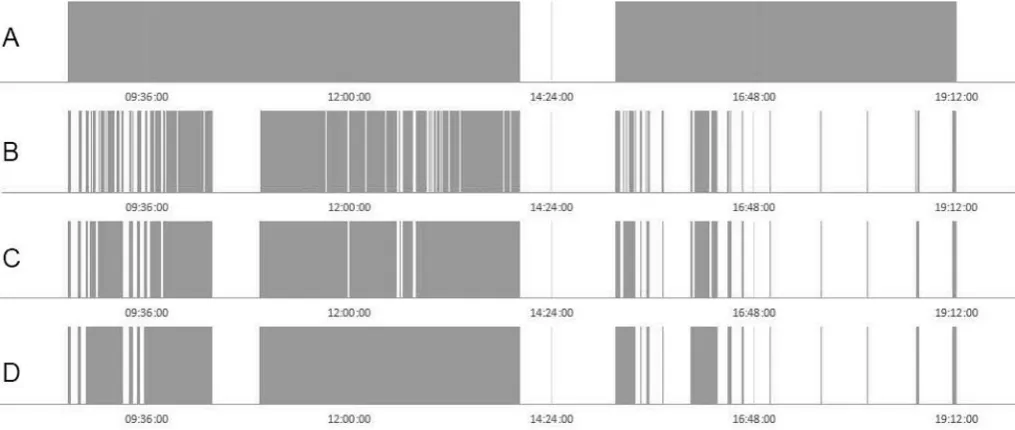
Fig. 7. Displaying the user-recorded (A) and sensor recorded (B) presence data across a sample day. Table 1

Comparison of modelled rooms.

Characteristic Modern Flat Victorian house

Volume 43.17 m3 _{44.86 m}3

Floor area 17.27 m2 _{17.95 m}2

Window area (Cardinal direction) 3.53 m2_{(E) 2.34 m}2_(S)

Glass U-value 3.004 W/m2_{-K 5.827 W/m}2_-K

Exterior wall area (Cardinal direction) 13.65 m2_{(E) 9.25 m}2_(S)

were treated as a continuous presence. Six different check window sizes were tested ranging from 30 s to 180 s, increasing in 30-s increments. A Raspberry Pi computer combined with a PIR motion sensor was set up in an office with 3 individuals working on computers and seated at desks. While people moved in and out of the office on a regular basis, it was unusual for the office to be empty except during a lunch break. Based on this, the assumption was made that presence fromfirst to last detection was constant.

The recorded office presence data spanned from 8:39 in the morning until 19:11 in the evening, with a gap from 14:01 to 15:10 when no-body was present.Fig. 5illustrates this time period in comparison with presence captured by selected check windows.

It is worth noting that the motion sensor positioning was not ideal. The sensor was located in the corner of the office, where two rows of

desks were positioned facing each other in the middle of the room. This meant that the sensor was behind one of the occupants and its vision obscured by computer screens for the remaining two. This explains the lack of data in parts of the morning and in the second half of the day -relatively subtle motions of hands and upper body associated with working at a computer were out of sight of the sensor, resulting in extremely low recorded presence in comparison to actual presence (15–55%).

In general, an increase in window duration corresponded to an in-crease in the percentage of actual presence time covered by the sensor data and a reduction in the number of data logging queries to the re-mote database, but too long a window would‘join’too many instances of motion detection and not reflect real life presence correctly.Fig. 6 plots the percentage of actual presence and the required queries as a function of window duration.

The percentage of correctly recorded presence time is asymptotic, with little improvement above 120s, beyond which there would be an increased risk of failure to adequately detect presence dynamics (ar-rival/departure times). Consequently (and supported by literature [25]), a 120s window was deemed adequate for deployment.

As noted earlier, this check window was further tested by installing the equipment (without heaters) in an open-plan kitchen/lounge of a 2-person household. The occupants of the house were asked to manually record the times they entered and exited the room, just as the sensor should over the course of a day.

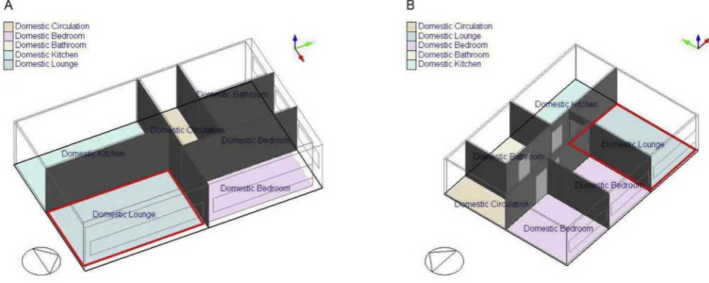
Fig. 7 plots the differences in manually recorded presences and those recorded by sensors. There were once again periods in the late afternoon where occupants were present but the sensor did not record them. This too was due to sensor placement–it can be speculated that occupants were watching TV or performing sedentary activities on sofas Fig. 8.Layout of modelled houses (A–Modernflat, B–Victorian house), with simulated rooms highlighted.

Table 2

Input assumptions relating to the four tested aspects of the control algorithm.

Process referred to Initial input assumptions

Presence Calculating the probability that a user is in the room, based on previous predictions and recorded presence.

An initial value of 0 was imposed for presence probability and recorded presence.

Slope Calculating a slope value for use in the optimum start algorithm.

An initial value of 1 was used for subsequent adjustment by the algorithm.

Temperature set-point Effects of user-provided feedback on thermal sensation votes for set-point temperature

An initial value of 10 °C was used. Vote casting was subsequently simulated by sampling from thermal sensation probability distributions corresponding to the current observed temperature, using the SCATS dataset [23].

Away schedules Users defining periods when they are away from the building to switch the heating off.

Two away schedules were built on days 19–21 and 113–119 to simulate the occurrence of

a weekend and a week from home.

Table 3

Describing, for the four tested aspects of the control algorithm the corresponding, input assumptions.

Configuration number House Heating system Algorithm setting

1 Modern Electric Maximise comfort

2 Modern Electric Minimise discomfort

3 Modern Central heating Maximise comfort

4 Modern Central heating Minimise discomfort

5 Victorian Electric Maximise comfort

6 Victorian Electric Minimise discomfort

7 Victorian Central heating Maximise comfort

8 Victorian Central heating Minimise discomfort

9 Modern Electric Control configuration

10 Modern Central heating Control configuration

11 Victorian Electric Control configuration

12 Victorian Central heating Control configuration

that were the furthest location from the sensor, causing slight posture changes to be missed.

There were also some false positives recorded by the sensor, but this may be due to short-lived entries to the room that were not recorded by the participants.

With a 120s window, the sensing equipment was only capable of recording 49.5% of the total presence duration. Based on this data, it would be unrealistic to assume that the algorithm would achieve a 0.8 probability of presence: the threshold above which we would deem occupants to be present. Therefore, assuming that around 50% of true presence would be captured, we set a threshold for the probability of presence of 0.4, in combination with the 120s window. If different, more reliable presence capture technology was intended to be used, this

value would need to be revisited.

2.1.2. Emulation method

Prior to deployment in thefield, the algorithm's functionality was assessed by simulating its output in an emulated environment, using EnergyPlus [4] coupled with the Building Control Virtual Test Bed (BCVTB) [6]. This setup allowed for different house models and algo-rithm configurations to be tested with ease.

representing two different house types (a purpose-built flat, and a Victorian house) and two different heating system types (electric heating & central heating) were used.Table 1summarises the diff er-ences in the modelled rooms between the two house types andFig. 8 present their layout.

These models are of two houses in Nottingham, UK with one oc-cupant simulated for each. In order to provide a representative depic-tion of the occupant's presence in the room, time use survey (TUS) data [8] was integrated. Collected during the year 2000, this TUS data de-scribes 20,981 people's activities in diary format at 10-min time steps. This was filtered to eliminate individuals younger than 18 years, wrapped to match the simulation start time of midnight (TUS diaries started at 4 a.m.) and grouped by weekday (so representing an average

adult's activities for each average day of the week). The data was thereafterfiltered to leave activities that the user reported to take place at home, and were likely to take place in the lounge. These included all reading-related activities, TV and video, radio & music, hobbies (in-cluding IT, arts etc.), socialising with household members, and house-hold management using the internet. Other activities were assumed to correspond to absence from the lounge.

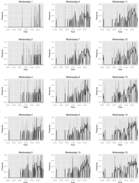
The simulation models used an ideal loads HVAC system: system capacity was constrained (1 kW for the electrical system and 3 kW for the thermal) and distribution losses and inertia was ignored, so that heat was delivered to the target zone(s) in an idealised way. This system was modelled in two configurations–one to simulate an electric con-vector heater (limited at a capacity of 1 kW zone sensible heating Fig. 10.Observed (grey) and predicted (line) presence probabilities: Wednesdays only, all configurations.

Fig. 11. (continued)

power) and another to represent a central heating system three times as powerful (3 kW capacity). Capacity limits were imposed to evaluate the usefulness of the algorithm's modelling of pre-heating start time. The simulation used Nottingham, UK weather data and was run fromfirst of January for 180 days (matching the estimated deployment time for the succeeding field trial, to capture the transition from full heating [winter], through partial heat to no heating [summer] demand). The assumptions made in initialising the control algorithm are outlined in Table 2below.

A control configuration was also included that utilised Energy Star recommended thermostat settings for a programmable thermostat [27]. The implemented settings utilised an occupant presence schedule be-tween 6am and 8am and 6pm-10pm with a 21 °C set-point temperature and 16 °C setback temperature at other times.

A total of twelve configurations were simulated, as illustrated in Table 3.

2.1.3. Emulation results

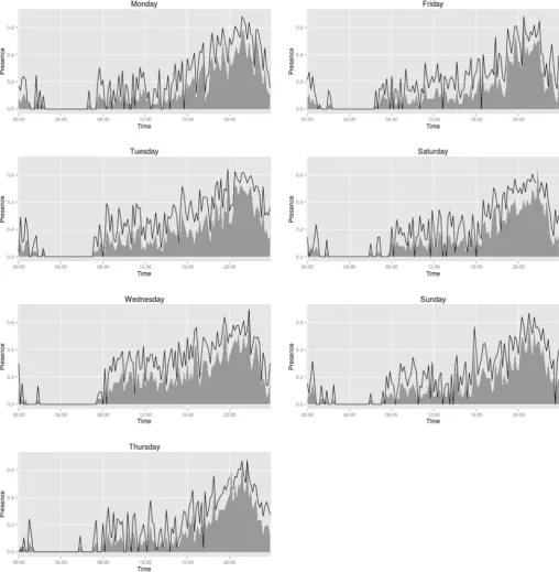
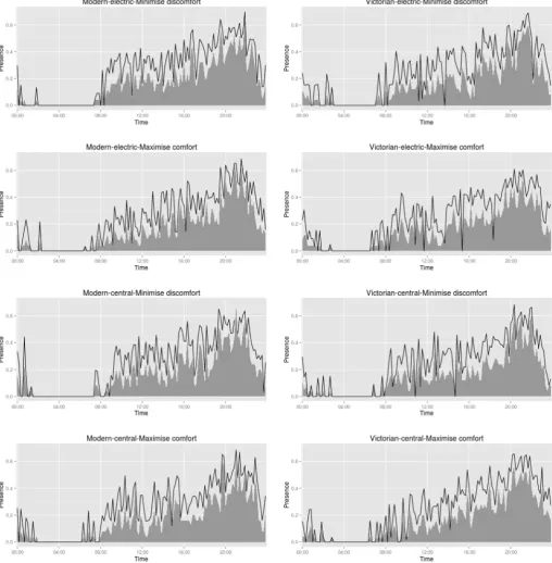
2.1.3.1. Presence prediction. Fig. 9depicts the algorithm's predicted and observed (TUS data) presence profiles for all days for the Modern-Electric-Minimise discomfort configuration and Fig. 10 compares Wednesday profiles for all configurations.

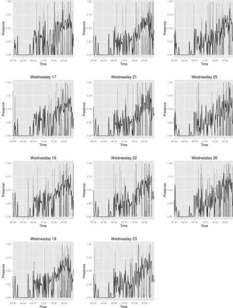
The algorithm was able to develop these profiles using only one week of training data, so that algorithm-scheduled heating periods were defined from the second simulated week onwards, indicating that the algorithm was relatively quick to learn new behaviours, highlighted in Fig. 11.

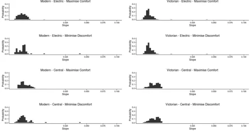
However, it is worth noting that this element was significantly in-fluenced by the simulated presence value. Within the simulation soft-ware, when a person was present in the room, the observed presence value for that 10-min time step would be 1 (meaning that presence is continuous throughout the timeslot). But in reality, our presence sen-sing apparatus may detect presence that began or terminated part way Fig. 12.Slope distribution for all simulated conditions (for clarity the x-axis has been clamped at 0.1, omitting the initial value of 1 and thefirst calculated instance of c0.2).

Fig. 14.Thermal sensation distribution (stacked area chart) with positive and negative temperature cumulative distribution functions (black lines) comparison between heating types.

Fig. 15.Thermal sensation distribution (stacked area chart) with positive and negative temperature cumulative distribution functions (black lines) comparison between heating control strategies.

through this time slot, so that partial presence would be recorded (a Real number rather than a Boolean); lowering the probability of a person being present and correspondingly increasing the number of historically similar day types needed for the threshold to be passed by which a meaningful presence would be predicted.

The mean observed (albeit based on Time Use Survey data in this emulation experiment) and predicted presence profiles presented in Fig. 10are a close match, suggesting that overall tendencies in occu-pation are captured well by our algorithm; albeit with systematic over-prediction (an error in magnitude) suggesting that the calibration parameters require further tuning, favouring historic predictions over recent observed presence (W in (1)). Naturally, the algorithm performs less well when comparing prediction with observation for specific days (Fig. 11). This is expected in an algorithm which is essentially using historical data to smooth (albeit with decay) perturbations arising from a process that is stochastic in nature. Nevertheless, these results do suggest that the weighting introduced a reasonable memory decay; so that the algorithm gradually adjusted itself to the latest behaviour trends.

The algorithm also successfully reproduces distinct presence profiles for each day of the week. While an individual weekday configuration makes the algorithm slower to adapt to abrupt but repeated (amongst similar day types) behaviour changes (due to a relative lack of training data for this weekday as opposed to using more abundant data for all weekdays), this sort of decay does support the handling of distinct differences in behaviour amongst similar day types. For example, for those working for a proportion of weekdays outside of their home.

Furthermore, with a RMSE of 0.363 in predicted presence prob-ability across all simulated use cases (flats, heating systems and prac-tices) and day types and with little variance (Monday 0.353, Tuesday 0.353, Wednesday 0.357, Thursday 0.358, Friday 0.363, Saturday 0.391, Sunday 0.393), the algorithm performs consistently throughout. Overall then, we suggest that the proposed algorithm performs adequately in predicting users' presence at home.

2.1.3.2. Slope. The slope in our optimal start algorithm represents the rate of increase of temperature in the room following activation of a heater. This variable is recalculated following every pre-heating

instance.Fig. 12depicts a distribution of all calculated slopes for all simulated conditions evolving from an initial value of 1. The results indicate that the algorithm quickly (within 2–3 instances) adjusted the initial value to reflect the building's characteristics (position on the x-axis).

It is clear from Fig. 12that the slope was rather stable but not constant, meaning that the optimum start algorithm (4) not only adapts itself to the fixed characteristics of the building (its envelope and construction materials), but also to the day-to-day variations in heat flows within the room, affected by thermal gains from occupants, out-door weather conditions, solar gains, heatflow to adjacent rooms, etc. These results suggest that the slope calculation and preheating func-tionality in the algorithm were both useful and functioned as expected.

2.1.3.3. Temperature set-point. Prior to any exploration of the results, it is important to note that the thermal sensation data used to simulate user voting was obtained from an experiment assessing occupants' thermal comfort in the summer. This is likely to cause a lower preferred set-point than might be expected for winter months, so that users may report being comfortable at temperatures that would otherwise seem unlikely or difficult to obtain via heating during winter months.

Figs. 13–15present the thermal sensation probability distributions obtained by drawing from observed distributions (SCATS data) for temperature bins matching those simulated, as well as the cumulative distribution functions of prevailing temperatures in the simulated en-vironment throughout the duration of the simulation; with the two curves intersecting at the median simulated temperature. Owing to limitations in heating capacity (1 kW electric, 3 kW central) for the houses of different standards of insulation (Modern insulated cavity wall, Victorian uninsulated solid wall) we observe considerable varia-tions in median temperature between housing type (a -Fig. 13) and more modest differences between heating system (b - Fig. 14) and strategy (minimise/maximise (dis)comfort strategies) (c -Fig. 15).

Interestingly, our different heating strategies led to very similar mean comfort votes (−1.1 for minimise discomfort, −1.0 for maximise comfort and−1.0 for the EnergyStar case).

On this basis, we conclude that the algorithm succeeds in adapting itself to users' thermal preferences and accommodates diversity in these preferences between housing and heating system configurations; with constraints on heating system capacity leading to offsets in median indoor temperature that are typically observed in poorly insulated housing.

2.1.3.4. Away schedules. Two away schedules were incorporated in the simulation and the effect of these can be seen inFig. 16. As explained in Fig. 1, the algorithm calculates a presence probability regardless of the away schedule. However, if the calculated time step falls within an away schedule, the set-point calculation is not executed, therefore preventing any heating activity from taking place.

Long periods of no heating activity can also be observed towards the

end of the simulation period, due to the relatively warm summer weather during which little or no additional heating was required.

From this we conclude that the algorithm performs as expected for the straightforward case of handling away schedules.

2.1.3.5. Energy implications. Finally, Fig. 17 compares performance criteria (energy demand, mean indoor temperature, and mean sensation) between all simulation configurations including the EnergyStar recommended programmable thermostat settings.

These results show that the proposed algorithm significantly out-performs the recommended (EnergyStar) programmable thermostat settings, reducing energy demand without compromising on comfort. The proposed algorithm delivered an average 45.8 kWhm−2_{saving in} comparison to a programmed schedule (average 68.8 kWhm−2for all EnergyStar conditions, average 23.0 kWhm−2 _{for all conditions).} Furthermore, the minimise discomfort algorithm configuration used on average 19.4 kWhm−2less energy than the maximise comfort condition Fig. 17.Energy and comfort implications comparison between all simulated conditions.

Table 4

Displaying the characteristics of the participating households (all names are pseudonyms).

Characteristics Flat 1 Flat 2 Flat 3

House exterior

Occupant characteristics and the anonymous persona assigned to them

Postgraduate student (male) - Carl 1 postgraduate student (male) - Paul, 1

professional (female) - Diane

2 postgraduate students (1 male - John, 1 female - Mildred)

Heating strategy Maximise comfort Minimise discomfort Minimise discomfort

App visibility Visible Blind Visible

Dwelling type Purpose builtflat Convertedflat Convertedflat

Rooms deployed with equipment 5 rooms–Lounge, Bedroom, Second

bedroom, Bathroom, Kitchen

4 rooms–Lounge/kitchen, Bedroom,

Bathroom, Hallway

3 rooms–Lounge/kitchen, Bedroom,

Bathroom

Existing heating system Gas central heating Electric convector heaters Electric convector heaters

Fig. 18.Floor plans highlighting the placement of sensor kits and heaters in the participating households (diagrams are not to scale).

(average 13.3 kWhm−2 _{for minimise discomfort, 32.7 kWhm}−2 _for maximise comfort), with simulated average thermal sensation votes only 0.1 lower on the ASHRAE 7-point scale (average vote of−1.1 for minimise discomfort, −1.0 for maximise comfort, −1.0 for EnergyStar). These results suggest that the energy use reduction oc-curred without an additional cost in user discomfort. However, these results relate only to simulations of single rooms with synthetic

representations of occupants. Nevertheless, the primary purpose of this simulation experiment was to evaluate the proof of principle of the algorithm, and that we believe we have done, rather than determine its absolute performance. For this we have conducted a real-life deploy-ment experideploy-ment, as set out below.

Fig. 20.Comparison of thermal sensation probability distributions with prevailing temperature positive and negative accumulative distribution functions (black) for participating households and their heating strategy.

2.2. Field deployment

2.2.1. Deployment method

Participants that satisfied the following criteria were self-selected. (1) They were responsible for their household heating expenses, (2) their existing heating system was preferably (but not limited to) elec-tricity based (ideally not storage heating), (3) they lived in a house/flat no bigger than 5–6 rooms, (4) apartments had to have a minimum of 2 rooms, and lastly, (5) occupants owned and used a smartphone running either an iOS or Android operating system. Recruitment for this study, which was based in Nottingham UK, was achieved through the aca-demic participant recruitment service callforparticpants.com,

university email mailing lists and the social media network Facebook. In total three households (seeTable 4for full detail) were recruited out of several that showed an interest.

temperatures to provide the algorithm with its initial conditions. Furthermore, interviews with participants were conducted 2 weeks after installation, 2 months into the experiment, and after its conclu-sion. Throughout the duration of the experiment, check-up emails were sent to the participants and daily check-ups utilising database queries and system logs were performed remotely. When delays in sensor data logging intervals occurred, the apparatus was remotely re-booted. In severe cases, participants were contacted to walk them through a manual restart by removing and replacing the power supply. With these measures, the installations were on-line for 87.5% (Flat 1), 56.4% (Flat 2, due to a poor internet connection for 2 rooms), and 82.3% (Flat 3) of the time. As noted earlier, participants were also sent reminder push notifications as prompts to submit thermal comfort votes. The rate of push notifications decayed over the course of the experiment from one in every two days in February, to every three days in March, and every four days subsequently until the end of the experiment. Following the conclusion of the experiment, participants were compensated with £20 Amazon shopping vouchers per month of participation.

2.2.2. Deployment results

In the following, we discuss the algorithm's performance in the participating households, who can broadly be described as “Fashion user”(Flat 1) characterised by the occupant's preference for selecting a desired clothing level and subsequently relying on the heating system to deliver thermal comfort, and ad-hoc working from home presence patterns;“Frugal user”(Flat 2) characterised by reported prioritisation of cost saving on heating (conflicting thermal preferences and strategies between occupants were also reported) and one occupant following a strict absence for work routine, while the other's work hours were flexible, creating variable presence-absence profiles; and“Everything's fine” users (Flat 3) characterised by their environmental conditions

naturally meeting their comfort expectations due to good insulation and high temperature gains from neighbouringflats, subsequently low en-gagement with the heating apparatus, and a strict absence for work pattern for both occupants. For more detail on the households and their interactions with the heating system and control application, please refer to Kruusimagi et al. [18].

2.2.2.1. Providing thermal comfort and user experiences for different heating strategies. Comparison of the maximise comfort and minimise discomfort heating strategies revealed that there was little difference between submitted average sensation votes - minimise discomfort 3.6 (on a 1 to 7 scale, or−0.4 on a−3 to +3 scale), maximise comfort 3.9 (minimise discomfort 108 votes by 4 users, maximise comfort 301 votes by 1 user). However, analysis of the reported values of how users felt and wanted to feel at the time (Fig. 19) between the two strategies showed that two dominant voting cases prevailed. In the first case, users reported a sensation of“cool”or“slightly cool”while they would have liked to have felt“neutral”or“slightly warm”. In the second case, users reported to have felt“slightly warm”or“warm”and would have liked to have felt a “neutral” or cooler sensation. Interestingly, the Maximise Comfort users had a higher probability of reporting thermal preference of“cold”at thermal sensations of“neutral”,“slightly warm”, or “warm” indicating that their heating strategy tended to deliver temperatures that were too high. In contrast, the Minimise Discomfort strategy users were more likely to feel“cold”, but their preference at the time tended to coincide with the Maximise Comfort users.

The‘fashion’and‘everything'sfine’users' households (top & bottom in Fig. 20) were within their comfort range (slightly cool/neutral/ slightly warm) for over 75% of the time. In contrast, the‘frugal’users' household (Fig. 20middle) experienced“cold”,“warm”or“hot” sen-sations for the same percentage of time. This appears to be in part due Fig. 22.Comparison of observed (colour) and predicted (line) average presence profiles in Flat 2 Room 4 (lounge) for all days.

to the users' operation of the system–limiting the amount of time it was turned on in order to save cost, thus choosing to subject themselves to such conditions.

While the results require verification from a larger sample size, these results do indicate that there is potential for utilising a minimise discomfort strategy as a nudging mechanism to reduce energy use without compromising on comfort; provided that occupants are in fa-vour of this strategy.

2.2.2.2. The ability to predict occupant presence and provide a spatiotemporal heating solution. The recorded presence data and system functionality logs showed that the algorithm was able to predict temporal variations in the profile of the probability of presence reasonably well (seeFig. 21comparing between rooms and Fig. 22comparing between days in the same room), particularly given the lack of training data, but the magnitude tended to be overestimated (suggesting once again that the weighting in equation(1)may need to be adjusted).

More specifically, we can identify in Fig. 21three rooms that are used intermittently but actively, and they are small enough that the motion sensor has a high hit rate. These are rooms Flat (F)1 Room (R)2, F2R1 and F3R2. We also observe rooms in which we reliably detect and thus predict presence during periods of activity and relatively poorly (over-predicting) during inactivity: F1R1, F1R5, F2R3, F3R3. Other rooms lie somewhat between these extremes. Furthermore, the diff er-ences between the days inFig. 22highlights that the algorithm creates a presence profile specific to the day of the week, adapting itself to the users' different activities regardless of the day.

Although our results are encouraging, it is worth noting that our ability to predict presence in this setup was constrained by the tech-nology used. Although this can be managed to some extent through calibration, we would recommend the use of more accurate sensing technology, also requiring a dedicated re-calibration check window and

presence thresholds. In a commercial application of our algorithm, these can be tailored to home configuration and user behaviours.

2.2.2.3. Algorithm adjusting to its environment and pre-heating in anticipation of occupancy. As noted earlier, our optimum start algorithm (OSA) aimed to calculate the most appropriate time to start pre-heating rooms for predicted presence. Owing to a combination of housing characteristics, the selected heating strategy and users' heating aspirations, there is a contrast in the number of instances in which heaters were activated; in particular when comparing F1 with F2 and F3 (see Fig. 23). Heaters were relatively frequently activated in F1 leading to a distribution of calculated slope parameters having a relatively small standard deviation. In contrast, heaters were seldom activated in the other houses (with the exception of F2R3), but when activated we do nevertheless observe a shift from the starting value of 1 towards lower values; indicating as observed during emulation process, that the algorithm successfully calculates a dynamic slope and the corresponding optimal start time (so long as the predicted presence probability is accurate).

2.2.2.4. Potential energy savings. Since no data was gathered regarding the participants' energy usage prior to the technological intervention (we used our own replacement heaters), it was not possible to demonstrate any energy savings directly. However, several promising results emerged.

A comparison of calculated neutral temperatures, based on reported sensation votes and coincident temperatures, with pre-study ques-tionnaire responses, revealed that households overestimated their pre-ferred set-point temperatures by some 2.1 °C (F1 = 1.71 °C, F2 = 4.3 °C, F3 = 0.32 °C). These results suggest that autonomous systems can po-tentially change households' heating system behaviours with corre-sponding energy savings.

participating households and all rooms, the heaters were switched on for an average of 1 h and 9 min per day (42min Everything'sfine user, 2 h 20min Fashion user, 25min Frugal user). These results were con-sistent with those of the simulated Modern Electric house, where heating operation times were 3 h 45 min (EnergyStar configuration), 1 h 32min (maximise comfort configuration), and 10min (minimise discomfort configuration). On average across the participating house-holds, this duration was just under the maximise comfort configuration in the simulation and suggests that an average saving of 46 kWhm−2 could be realised in comparison with the EnergyStar recommended programmable thermostat settings over half a year. But, these results are somewhat speculative. An accurate assessment would require measurements of energy use (and preferably also indoor and outdoor– for normalisation purposes–conditions), both pre- and post-interven-tion.

3. Conclusions

The aim of this exercise was to evaluate thefitness for purpose and real life performance of a quasi-autonomous spatiotemporal home heating control algorithm.

Our results suggest that the proposed algorithm was able to develop a presence profile for a single room for every day of the week in both emulated and true-to-life environments. While the proposed algorithm is relatively simple in its logic in comparison to more complex presence prediction solutions ([28] or [22]), and could be further improved upon using more reliable sensing technology, we do accommodate real-life diversity, which has been demonstrated in thefield study. Our algor-ithm's memory decay allows it to perform well in changing conditions and to adapt itself to interpersonal differences in thermal preference. In the version presented here, memory decay was not applied to thermal preference or set-point calculation, but this could readily be accom-modated. In addition, we have shown that our algorithm was able to adapt itself to its environment; to the building envelope, heating system specifications, daily changes in climate conditions. Our algorithm is able to achieve this level of operation and performance with virtually no training data. We believe this to be of paramount importance for systems designed for the home setting.

Our evaluation of both maximise comfort and minimise discomfort strategies suggest that heating control algorithms can proactively nudge users towards more energy efficient behaviours without compromising comfort requirements. This calls for testing of other domestic algo-rithms in the wild, where their core functionality can be coupled with users' behaviour and preferences, and thus for the system to be assessed from a holistic joint-cognitive systems view, ensuring a pleasurable user experience while allowing for a higher degree of granularity in spa-tiotemporal heating control and corresponding energy savings.

Acknowledgements

The authors acknowledge Jacob Chapman and Daniel Ratzinger for their invaluable input in the realisation of this project. The study was approved by University of Nottingham Faculty of Engineering ethics committee. This work was supported by the Engineering and Physical Sciences Research Council [grant number EP/G037574/1].

References

[1] ASHRAE, ASHRAE Standard 55.66: Thermal Comfort Conditions, (1966).

[2] A.B. Birtles, R.W. John, A new optimum start control algorithm, Build. Serv. Eng. Technol. 6 (3) (1985) 117–122 1985.

[3] Department of Energy & Climate Change, Energy Consumption in the UK - Chapter 1: Overall Energy Consumption in the UK since 1970, (2014).

[4] EnergyPlus | EnergyPlus,https://energyplus.net/, (2016) , Accessed date: 4 March

2016.

[5] EWMA Excel | Exponentially Weighted Moving Average | Reference Manual |

NumXL,http://www.spiderfinancial.com/support/documentation/numxl/

reference-manual/descriptive-stats/ewma, (2015) , Accessed date: 13 May 2015.

[6] FrontPage, bcvtb,https://simulationresearch.lbl.gov/bcvtb, (2016) , Accessed date:

4 March 2016.

[7] G. Gao, K. Whitehouse, The self-programming thermostat: optimizing setback schedules based on home occupancy patterns, Proceedings of the First ACM Workshop on Embedded Sensing Systems for Energy-efficiency in Buildings, 2009, pp. 67–72 2009.

[8] J. Gershuny, et al., Multinational Time Use Study, Versions World 5.5.3. 5.80 and 6.0. Centre for Time Use Research, University of Oxford, United Kingdom, 2011. [9] A. Ghahramani, et al., Energy savings from temperature setpoints and deadband:

quantifying the influence of building and system properties on savings, Appl. Energy 2016 (2016).

[10] I. Griffiths, Thermal comfort studies in buildings with passive solar features, Field Studies. Report to the Commission of the European Community, ENS35, vol. 90, 1990 1990.

[11] M. Gupta, et al., Adding gps-control to traditional thermostats: an exploration of potential energy savings and design challenges, Pervasive Computing 2009 (2009) 95–114.

[12] E. Hollnagel, D.D. Woods, Joint Cognitive Systems: Foundations of Cognitive Systems Engineering, (2005).

[13] F. Jazizadeh, et al., Human-building interaction framework for personalized thermal comfort-driven systems in office buildings, J. Comput. Civ. Eng. 2014 (2014).

[14] R. Kannan, N. Strachan, Modelling the UK residential energy sector under long-term decarbonisation scenarios: comparison between energy systems and sectoral mod-elling approaches, Appl. Energy 86 (4) (2009) 416–428 2009.

[15] W. Kleiminger, et al., Smart heating control with occupancy prediction, The 2014 ACM International Joint Conference, 2014 2014.

[16] C. Koehler, et al., TherML: occupancy prediction for thermostat control, Proceedings of the 2013…, 2013 2013.

[17] J. Krumm, A.J.B. Brush, Learning Time-based Presence Probabilities. Pervasive Computing, Springer, 2011, pp. 79–96.

[18] M. Kruusimagi, et al., Living with an autonomous spatiotemporal home heating system: exploration of the user experiences (UX) through a longitudinal technology intervention-based mixed-methods approach, Appl. Ergon. 65 (2017) (2017) 286–308.

[19] G.J. Levermore, Building Energy Management Systems: Applications to Low-energy HVAC and Natural Ventilation Control, Taylor & Francis, 2000.

[20] J. Lu, et al., The smart thermostat: using occupancy sensors to save energy in homes, Proceedings of the 8th ACM Conference on Embedded Networked Sensor Systems, vol. 2010, 2010, pp. 211–224.

[21] A. Majumdar, et al., Energy-comfort optimization using discomfort history and probabilistic occupancy prediction, 2014 International Green Computing Conference, IGCC 2014, 2015 2015.

[22] M.C. Mozer, et al., The neurothermostat: predictive optimal control of residential heating systems, Adv. Neural Inf. Process. Syst. 1997 (1997) 953–959. [23] J.F. Nicol, K.J. McCartney, SCATS: Final Report. Technical Report, Oxford Brookes

University, Oxford, 2001.

[24] R.K. Pachauri, et al., Climate Change 2014: Synthesis Report. Contribution of Working Groups I, II and III to the Fifth Assessment Report of the Intergovernmental Panel on Climate Change, IPCC, 2014.

[25] J. Page, et al., A generalised stochastic model for the simulation of occupant pre-sence, Energy Build. 40 (2) (2008) 83–98 Jan. 2008.

[26] J. Palmer, et al., Great Britain's Housing Energy Fact File 2011, DECC, London, 2011 2011.

[27] Programmable Thermostats |ENERGY STAR,https://www.energystar.gov/

products/heating_cooling/programmable_thermostats, Accessed date: 4 June 2016. [28] J. Scott, et al., PreHeat: controlling home heating using occupancy prediction,

Proceedings of the 13th International Conference on Ubiquitous Computing (New York, NY, USA, 2011), 2011, pp. 281–290.

[29] UK Parliament, Climate Change Act 2008. The Stationery Office Ltd., London. March (2008), (2008).

[30] WIFIPLUG - App controlled smart plug - App controlled Smart Plug - WiIFIPLUG: http://www.wifiplug.co.uk/. Accessed: 2016-01-20.