Does the composition of government expenditure matter for long run GDP levels?

For Peer Review

Does the composition of government expenditure matter for long-run GDP levels?

Journal: Oxford Bulletin of Economics and Statistics Manuscript ID: OBES-09-113.R5

Manuscript Type: Original Article

For Peer Review

Does the composition of government expenditure matter for

long-run GDP levels?

NORMAN GEMMELL

_{RICHARD KNELLER}

_{ISMAEL SANZ}

‡_{Victoria Βusiness School, Victoria University of Wellington, New Zealand}

(Corresponding author: e-mail: [email protected])

†

School of Economics, University of Nottingham, UK (e-mail: [email protected]) ** Universidad Rey Juan Carlos. Madrid, Spain.

(e-mail: [email protected])

Abstract

We examine the long-run GDP impacts of changes in total government expenditure and in the shares of different spending categories for a sample of OECD countries since the 1970s, taking account of methods of financing expenditure changes and possible endogenous relationships. We provide more systematic empirical evidence than available hitherto for OECD countries, obtaining strong evidence that reallocating total spending towards infrastructure and education is positive for long-run output levels. Reallocating spending towards social welfare (and away from all other expenditure categories pro-rata) may be associated with modest negative effects on output in the long run.

Word count: 11.961

JEL codes: H50; O40

Keywords: government expenditure composition, fiscal policy, GDP

This version: August 2015

For Peer Review

I. Introduction

The fiscal stimulus packages enacted in many countries from 2009 onwards to combat the global economic crisis typically included changes in various public expenditure programs. Much debate surrounded the merits of these fiscal packages, not least with respect to the wisdom of governments’ attempts, and ability, to stimulate the economy via expenditure injections. The specific public spending choices in these short term fiscal packages were motivated in part by a desire to be consistent with long term growth objectives, such as expanding infrastructure spending perceived as benefiting long-run GDP levels or growth rates. The austerity programs that have been used since then to deal with the resulting high levels of public debt have led to the same debates but from the opposite side; which types of expenditure should be cut and what are the longer term growth effects from doing so. This brings to the fore the twin questions: how strong is the evidence that long-run income levels or growth rates respond to public expenditure changes, and which expenditure categories have greatest impact?

This paper focuses on these two questions. We first briefly review the relevant theory. This builds on Barro (1990) and Devarajan et al. (1996) who proposed that some ‘productive’ public

expenditures can influence long-run growth rates via public sector inputs in private production functions. Following a brief discussion of the existing evidence on long-run public expenditure-output relationships, we provide more systematic empirical evidence than available hitherto for OECD countries.1

In addition to the above political economy motivations, there are a number of academic reasons to re-examine this issue. Firstly, most empirical studies focus on a subset of individual expenditure categories, such as defence, education or transport and communication expenditures. These have produced a mixed set of findings and do not typically allow the trade-offs between different forms of public expenditure to be identified explicitly. Our approach provides evidence on these trade-offs.

Secondly, a number of recent papers have used alternative methodologies to examine long-run impacts of tax policy on GDP levels or growth rates (see Adam and Bevan, 2005; Lee and

Gordon, 2005; Romero-Avila and Strauch, 2008; Arnold et al, 2011; Gemmell et al., 2011,

2015). However, public expenditure is rarely the primary focus of attention in these studies, or

it is tested as an aggregate ‘productive’ spending category. In this paper we limit attention to potential effects of public expenditures on long-run GDP levels, focusing both on total public expenditure (suitably financed via the government budget constraint) and specific functional spending categories.

1 _{We abstract from the question of whether there are short-run benefits from stimulus packages, analysis of which}

requires quite different empirical methodologies.

For Peer Review

Thirdly, dealing with endogeneity associated with estimates of fiscal impacts on GDP has proved difficult in previous studies. While we do not claim to have resolved these concerns in this paper, we do carefully address potential endogeneity problems. Our fiscal variables would appear to be at least ‘weakly exogenous’ (based on standard econometric definitions, see Johansen, 1992, and Boswijk, 1995) with respect to their estimated effects on GDP.

Fourthly, use of panel data methods has increased the reliability of recent studies. However, these generally use fixed effects estimators which impose parameter homogeneity across countries. Furthermore, as Haque’s (2004) re-examination of the Devarajan et al (1996)

results shows, how the time-series properties of the data are handled can be crucial for estimated output effects of fiscal variables.

In this paper, access to an extended panel dataset with a longer time dimension than previous studies has permitted application of the more flexible Pooled Mean Group (PMG) estimator proposed by Pesaran et al. (1999). This enables us to explore both short run dynamics

and long-run equilibrium relationships among the variables of interest, and account for heterogeneity across countries in their short run dynamic relationships. We compare these results with those obtained using more restrictive dynamic fixed effects (DFE) methods, and the more flexible, but data-intensive, Mean Group (MG) approach.

These improvements provide more robust evidence on the potential long-run association and causation between public spending and GDP. This supports some traditional views, such as that a spending reallocation towards infrastructure and education spending (and to a lesser extent, health) can raise GDP over the long run. Our results also suggest that, relative to public spending ‘on average’, social welfare spending may have moderate GDP-reducing effects. This implies a possible trade-off between public spending aimed at income redistribution via social welfare spending, and spending aimed at raising overall income levels.

The remainder of this paper is structured as follows. Section II briefly describes the links between public expenditure composition and GDP growth hypothesised by recent theory, and summarises current evidence for OECD countries. Section III then discusses our testing methodologies and dataset; while section IV reports results for a sample of 17 OECD countries over 1972-2008. Some conclusions are drawn in section V.

II. Public spending, taxes and growth

Theory

As is well known, in the neoclassical growth model, if the incentives to save or to invest in new capital are affected by fiscal policy, this alters the equilibrium capital-output ratio, and therefore the level of the output path but not its slope. There are effects on growth rates only for

For Peer Review

a transitional period as the economy moves onto its new output path, though the length of this transition remains subject to debate.2 _{There is, however, a resulting permanent impact on the} long-run level of output (GDP). The 1990s saw the development of a number of growth models

with a permanent, or at least persistent, role for fiscal policy such as those of Barro (1990), Futagami et al. (1993) and Deverajan et al. (1996).

A novel feature of these models was that fiscal policy can determine both the level of the output path and the steady-state (long-run) growth rate.3 _{Key fiscal aspects include some} ‘productive’ public expenditures affecting private sector productivity while other ‘unproductive’ expenditures only impact on citizens’ welfare (including the possibility of zero welfare effects), and that some taxes levied to fund public expenditures distort investment decisions. In a model with multiple productive expenditures Devarajan et al. (1996) show that

the long-run growth effects depend upon a combination of the relative productivities of these

expenditures and their relative budget shares.

A number of recent papers have modelled the relationship between particular public spending categories and growth. For example, Blankenau and Simpson (2004), Agénor and Neanidis (2006), Semmler et al. (2007), Agénor (2008) and Agénor (2012) have examined

various extensions of the Barro/Devarajan framework which explicitly model infrastructure, education and/or health spending as inputs into private production; and interactions between these spending types. For example, health services or infrastructure spending may enter the production function for education.4

These models propose mechanisms by which permanent impacts on GDP growth rates can arise in association with changes in particular public expenditure categories, especially those related to infrastructure and human capital production. However, permanent growth effects in these endogenous growth models generally depend on so-called ‘knife-edge’ properties whereby reproducible factors of production must display exactly constant returns to scale (Solow, 1994; Dalgaard and Kreiner, 2003). While the conditions for such permanent effects may be restrictive, and hard to verify empirically, even in their absence, the mechanisms embedded in endogenous growth models suggest that public spending could have effects on growth that are highly persistent.

Existing empirical evidence on public expenditure and growth

2 _{Turnovsky (2004), for example, estimates ‘transitional’ output adjustments to fiscal policy changes in terms of}

decades, while Lee et al. (1997) find convergence to equilibrium with half-lives of a few years, rather than

decades.

3 _{Not all endogenous growth models predict long-run growth effects from fiscal policy, such as the ‘non-scale’}

growth model of Eicher and Turnovsky (1999).

4 _{See Albertini}

et al. (2014) for an examination of short-run fiscal multipliers for different components of

government spending at the zero lower bound, based on a New Keynesian model.

For Peer Review

Much of the empirical literature testing for fiscal policy impacts on long-run GDP levels or growth rates suffers from various methodological weaknesses.5 _{In particular it is now} recognised that tests of the output effects of public expenditure decompositions (and other fiscal variables) must accommodate the total government budget (expenditures, revenues, deficits); a feature missing from much of the earlier literature. Nevertheless, for specific spending decompositions, some early studies found education, health and/or transport & communication (T&C) spending to be positively associated with GDP growth; see Nijkamp and Poot (2004) for a meta-analysis of early studies.

As shown by Kneller et al. (1999), without accounting for the government budget

constraint (GBC), evidence on the long-run output effects of public expenditures is difficult to interpret and can appear to be non-robust. Recent studies, such as Acosta-Ormaechea and Morozumi (2013) and Afonso and Jalles (2014), have sought to accommodate the GBC, to varying degrees, in their empirical approaches. Both studies focus on social security, education and health spending (and T&C in the case of Acosta-Ormaechea and Morozumi), generally finding negative associations between GDP growth and social security spending but positive associations for education and health. These results are obtained for large samples of developing and developed countries, rely on period averaging of annual data (hence ignoring short-run dynamics), and impose parameter homogeneity across countries.

As noted above, we prefer to focus on a more homogeneous group of OECD countries, using annual data and panel techniques that can identify both short and long-run effects whilst allowing for heterogeneity across countries in responses to fiscal shocks. Like Acosta-Ormaechea and Morozumi (2013), and Arnold et al.’s (2011) analysis of tax decompositions,

we examine relationships between fiscal variables and long-run GDP levels rather than growth

rates. An advantage of this ‘levels specification’, discussed further below, is that it allows the data to identify the degree of persistence in GDP growth responses, rather than impose a functional form embodying permanent effects.

III. Methodology and data

Growth versus level effects

The empirical specification adopted by much of the empirical literature testing for public expenditure-GDP growth effects since Devarajan et al. (1996) is based on their endogenous

growth model. This model, derived from the Barro (1990) framework, essentially generates an estimating equation in which the growth rate of GDP in country i at time t is a function of the

ratio of total government expenditure, E, to GDP and a vector of shares of j individual

5 _{See Slemrod (1995), Tanzi and Zee (1997), Myles (2000) for earlier, more detailed reviews and Temple (1999)}

for a more wide-ranging review of growth empirics.

For Peer Review

categories within total government expenditure, ej. Sets of conditioning variables, consistent

with a more general growth model or more pragmatic considerations, are often included; see Devarajan et al. (1996; p.322). In a panel context, the Devarajan et al. endogenous growth

model takes the form:

(

)

(

)

1 ,

, =∆ = +

∑

k k t

i t

i t

i y E Y E E

g

β

β

µ

ω

ε

where yit is the log of GDP per capita in country i at time t, git is the growth rate (log difference:

it

y

∆ ), Y is GDP, E is total public expenditure and Ek is the kth expenditure component, µi and ωt

are country and time fixed effects, and εit is a classical error term.6

A difficulty with equation (1) is that it is specific to the endogenous growth model with permanent growth effects from fiscal policy changes, and no transitional dynamics. To allow for Solow-type transitional dynamics, but where the effects of fiscal policy may be persistent, requires a more flexible functional form. This is particularly important when working with annual data. We follow Arnold et al. (2007, 2011) and use an autoregressive distributed lag,

ARDL(p, q), model, parameterised in error correction form.7 This allows both the short run

dynamic, and the long-run equilibrium, relationships between GDP and fiscal variables to be separately identified.

Consider the following general ARDL(p, q) specification:

, = ∑,, + ∑,, + +, (2.1)

∆, =ζ∆, +ζ∆, + … +ζ∆, + , (2.2)

where the vector Xi,t in (2.1) includes both the fiscal variables of interest (e.g. the level and mix

of expenditures, E/Y and Ek/E respectively), and control variables. The α, β, and ζ are parameters to be estimated; where the ζs capture the autoregressive process in ∆Xi,t.

A number of parameterisations of (2.1) are possible (see Wickens and Breusch, 1988), but it is convenient to express (2.1) in error correction (ECM) form:

, = ∆, =φ, − , + ∑,∗ ∆, + ∑,∗ ∆, + +, (3)

where φ = −(1 − ∑_,) captures the error correcting component, and = (∑ ,/φ)

captures the long-run equilibrium relationships between y and X, with short run effects

measured by ,∗ – the parameters associated with the ∆X variables in (3). The error correction

term, φi, is a measure of the speed at which the model returns to equilibrium after a shock.

Equation (3) allows φi, and βi, to vary across countries, though alternative econometric

6 _{The dependent variable in some cases is per capita GDP growth, which simply involves a re-parameterisation}

when GDP is on the left-hand side and the vector of control variables includes a measure of population growth on the right-hand side.

7_Arnold

et al. (2007) show that such a specification can be consistent with, and nest, alternative augmented Solow

and (Uzawa-Lucas) endogenous growth models.

For Peer Review

approaches (PMG, MG, DFE etc.) involve differing homogeneity restrictions, as discussed further below.

The degree of persistence of any fiscal effects on output growth in the model is, of course,

determined by the model’s convergence properties.8 _{Although the dependent variable in (3) is} per capita GDP growth, the regression measures the impacts of fiscal and other variables on the

long-run per capita GDP level, since (3) is merely a re-parameterisation of (2.1).

The government budget constraint

Since the GBC describes a ‘closed system’, whatever parametrisation is adopted the estimating equation needs to recognise that expenditures, Ei,t, must be financed by revenues,

Ri,t, and/or the budget surplus/deficit, Di,t, each with potential output effects, since D_it=R_it−E_it

(see Kneller et al., 1999; Gemmell et al., 2011). As a result, in addition to the variables E/Y and

∆(E/Y) within the vectors X and ∆X in (3), (R/Y) and (D/Y) also potentially have effects on

output with any net output effect depending on the particular financing combinations assumed. Hence a decomposition of βiXi,t in equation (3) includes (setting βi = β for convenience):

(

)

(

)

(

)

(

)

... _{1 ,−1}+ _{2 ,−1}+ _{3 ,−1}+

_∑

k

t i k t

i t

i t

i R Y D Y E E

Y

E

β

β

β

β

and similarly for the short run output effects of expenditures, revenues and deficits. However, since introducing all three variables would be perfectly collinear in a regression, one must be chosen to omit. Omitting (D/Y)i,t-1, (4) becomes:

(

)

(

)

(

)

) (

... ₁− _{3 ,−1}+ ₂− _{3 ,−1}+

_∑

k

it k t

i t

i R Y E E

Y

E

β

β

β

β

β

This demonstrates the correct interpretation of the output effects of expenditure and revenue variables, within this model. Estimates of the fiscal parameters in (5) capture the effects of increases in total expenditure, or decreases in revenues, financed by changes in the budget deficit (the omitted category in this example). These effects can be seen to depend on the signs and relative sizes of β1, β2 and β3. In comparison, the interpretation of the coefficients

on the individual expenditure share components of interest, β4,k, remains unaffected.

In the applications below, each regression includes one of the k = 1…K expenditure share

elements, Ek/E, where the included kth expenditure category is rotated across the K different

categories. Including each expenditure share in turn, rather than all K-1 expenditure shares

simultaneously, saves on degrees of freedom in our panel regression model which requires a large number of parameters to be estimated; see below.9

8 _{Though the parameter φ can be interpreted as a speed of adjustment, it is not equal to the more familiar rate of}

conditional convergence in this model. This is because the short-run dynamics are more complicated than in a conditional convergence regression.

9 _{By repeating regressions on equation (3) but including a different expenditure category each time (from (5)), the}

per capita GDP impacts of a bilateral switch between any two expenditure categories, l and m, can be obtained. 1

For Peer Review

We estimate an equation of the form in (3) above using the pooled mean group (PMG) methodology of Pesaran et al. (1999), and compare this with the equivalent results using fixed

effects (FE), and mean group (MG), estimators. The PMG estimator provides a useful intermediate alternative between estimating separate country regressions (the MG case) and the fixed effects estimator which imposes homogeneity on all slope coefficients and error variances across countries. The PMG estimator allows the intercepts, short run coefficients and error variances to differ freely across groups, but constrains the long-run coefficients to be the same.

If homogeneity of the long-run responses is not rejected, the PMG is the preferred estimator because of its efficiency relative to the MG estimator which permits long-run heterogeneity. Pesaran et al. (1999) demonstrate that the PMG’s allowance for short run

parameter heterogeneity yields more reliable estimates of the long-run responses, and can affect estimated speeds of convergence towards long-run equilibrium.

A disadvantage of the PMG estimator is that, unless the available time series are long, a degrees of freedom problem is soon reached. For the dataset available here this requires some restrictions on lag lengths and/or the set of right-hand-side (RHS) variables. For this reason we restrict the RHS variables to include each expenditure share separately in turn, with up to two lags. Though this lag length is relatively short, inclusion of the lagged dependent variable ensures the specification can accommodate a high degree of persistence in the short run adjustment process following a shock.

We also include two non-fiscal control variables – the private non-residential investment rate and employment growth. These variables appear in many empirical growth models capturing the role of private sector inputs. Also, recognising that some public expenditures may impact on GDP partially through their impact on private investment, we omit the latter variable from some specifications.

An important aspect of equation (3) when testing for the output effects of public expenditures is that it allows the degree of persistence of these effects to differ across expenditure types, at least to the extent that these can be captured by the 30+ years of our data. In addition, we test the PMG assumption of long-run parameter homogeneity against the mean group (MG) and fixed effects (FE) alternatives, using a Hausman test.

Addressing endogeneity

A major concern when running regressions of the form in (3) is, of course, the potential for simultaneity between GDP per capita and the right-hand-side variables − especially the fiscal and investment variables, a point stressed by Slemrod (1995) in a cross-section growth

For Peer Review

regression context. In addition, country-specific, time-varying factors such as changes to political and institutional settings may influence both fiscal policy and GDP per capita.10 These may be compounded by persistence in the annual fiscal series and potentially long lags in the impacts of fiscal variables on GDP per capita, generating serial correlation in the error process that must be dealt with adequately. As a result the fiscal variables of interest here may be endogenous, with well-known problems of interpretation for the short and long-run OLS parameters.

In a series of papers in the mid-1990s, Pesaran and associates (see, for example, Pesaran and Smith, 1995; Pesaran, 1997; Pesaran and Shin, 1999) demonstrated that, under a number of conditions such as a unique cointegrating relationship, estimates of the long-run parameter vector, ββββ, obtained from OLS regressions of models such as (3) are consistent.11 _{Further, based}

on simulation results, Pesaran et al. (1999) demonstrate that even in small samples standard

t-and F-tests on the long-run parameters from the ECMs are valid, given suitable specification of

the lag structures of dependent and independent variables.12

Further, where serial correlation is a concern, ‘appropriate modification of the orders of the ARDL model’ (Pesaran and Shin, 1999, p.386) is sufficient to deal with both the serial correlation in the error process and/or regressor endogeneity (see also Kanas and Kouretas, 2005). We discuss these aspects further in section IV when we present our empirical results.

The updated dataset

Results reported below are based on an extension of the Bleaney et al. (2001) dataset, which

uses the IMF’s Government Financial Statistics (GFS) fiscal data for 17 OECD countries to construct measures of total expenditure and individual expenditure shares, distortionary and non-distortionary taxes, and budget surpluses/deficits.13 _{The original data, available from the} early 1970s to 1995, have been updated to 2007 or 2008, providing around 30-35 annual time-series observations each for most of the 17 countries.14 _{We exclude data after 2008 to avoid} long-run estimates being unduly affected by the large shock (associated with the global financial crisis and its aftermath) to fiscal, GDP and other variables after 2008.

Data on GDP, the private investment/GDP ratio and employment growth were obtained for the same period from OECD sources. An important difference from previous studies is that our investment variable is private non-residential investment (PNRI) instead of total investment

10 _{We do however deal with time-specific shocks common to all countries in the sample.} 11 _{Indeed, where variables are I(1), they argue that parameter estimates are super-consistent.} 12 _{See, for example, Pesaran (1997, pp. 182-185), Pesaran and Shin (1999, pp. 381-387; 404-405).}

13 _{The 17 OECD countries are Australia, Austria, Canada, Denmark, Finland, France, Germany, Iceland,}

Luxembourg, Netherlands, New Zealand, Norway, Spain, Sweden, Turkey, UK and US. Other OECD countries are excluded due to missing values for several years; see online appendix.

14 _{This is not straightforward, however, because of changes in the GFS methodology, which moved from a cash}

accounting, to an accruals accounting, basis for fiscal data from the late 1990s onwards; see online appendix.

For Peer Review

(gross fixed capital formation). Since all regressions include various public expenditure variables, the use of PNRI avoids the possibility of double counting much public investment which otherwise would contribute to both the investment and public expenditure data. Before running all regressions we de-mean all data series as recommended by Lee et al. (1997) and

Pesaran et al. (1999) to deal with potential cross-sectional error correlation. Measuring all

variables as deviations from their sample means in each year removes the effects of common shocks in the data.

IV. Empirical results

Pre-testing for lag lengths

As discussed in section III, following Pesaran and Shin (1999), regressions on equation (3) require knowledge of the appropriate lag structures if the Xi,t in (3) are to be interpreted as

exogenous or weakly exogenous; see below. Before running our PMG regressions, our procedure therefore follows the pre-test proposed by Pesaran and Shin (1999) to select the preferred lag structure for the dependent, and each independent, variable based on the Schwarz Information Criterion (SIC; see Pesaran and Shin, 1999). This uses up to two lags for each variable and country; in practice we find that two lags are required relatively rarely.15 _The results of PMG regressions on equation (3) reported below are those for the SIC-based lag structures.

Testing for total public expenditure effects

Before examining the GDP effects associated with the shares of particular expenditure categories it is worth noting the impact of the omitted financing category in the government budget constraint because it affects the interpretation of the included parameters. As the parameter estimates on the shares of individual spending categories in total expenditure are unaffected by this we omit them from the regressions for the moment.

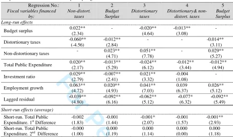
Table 1 shows the long-run and short run parameters for six PMG regressions in which total spending is included, financed by combinations of three alternative fiscal variables (non-distortionary taxes, deficits and (non-distortionary taxes) in columns 1-4. Column 5 repeats the regression in column 2, but with the private investment control variable omitted.16 _{Results for} alternative (MG and DFE) estimators are then reported in Table 2. The role of different implicit

15 _{For example, in each of regressions 1–3 of Table 1, there are a maximum of 204 possible parameters (17}

countries x 6 included variables x 2 lags). Regression 4 involves 5 variables, hence 170 possible parameters. For

those four regressions, two lags were selected in only 11%, 8%, 9% and 4% respectively of the possible cases.

16 _{In general the ‘non-distortionary’ taxes in this context are consumption taxes. The term ‘less growth}

distortionary’ may be more appropriate in this case since these taxes can distort investment decisions in models where labour supply effects are allowed for. The method of aggregating the GFS functional classification into these sub-aggregates is described in Bleaney et al. (2001). ‘Other revenues’ refers to the GFS categories ‘taxes on

international trade and transactions’, ‘other taxes’ and ‘non tax revenues’. It is unclear how distortionary these might be. Other revenues (non-tax revenues) are approximately 13% (9%) of total revenues in our sample.

For Peer Review

financing of fiscal variables has been discussed by Gemmell et al. (2011) so is only briefly

reviewed here.

[Table 1 about here]

Regression 1 in Table 1 reveals that increasing total public spending, financed by the (omitted) non-distortionary taxes has a long-run output effect that is positive and statistically significantly different from zero. However, the same spending increase can alternatively be financed by either a reduced budget surplus (regression 2), or by an increase in distortionary taxes and/or increases in any/all taxes (regressions 3 and 4), or by some combination. Regressions 2-4 in Table 1 show that each of those cases produces a negative, statistically significant long-run parameter on the public expenditure variable. The different regression specifications in Table 1 confirm that the assumed (or imposed) method of financing a public expenditure increase is crucial for estimates of their likely impact on long-run levels of GDP per capita.

The Table 1 results suggests that, within our dataset, use of ‘non-distortionary’ forms of taxation (such as VAT) to fund a given unit of additional public spending has been associated,

ceteris paribus, with increases in GDP per capita levels in the long run, whereas other forms of

financing such spending have been associated with decreases in GDP per capita.17 _{Table 1} results for total public expenditure parameters also tend to suggest that the adverse long-run effects on GDP per capita from distortionary tax financing (at –0.024) are significantly greater than those associated with other forms of financing (around –0.012).18 However this should be interpreted cautiously. As we show below, specifications that also allow for different effects on GDP per capita from differences in specific public expenditure shares (Table 3) suggest that the magnitude of the total expenditure parameter can be somewhat sensitive to the included expenditure share variables.

Recognising that some fiscal-GDP effects could be mediated through private investment (as distinct from via factor productivity), regression 5 in Table 1 examines whether omitting investment from the control variables affects conclusions regarding the GDP impacts of public expenditures. Comparing the equivalent, budget deficit-financed cases in regressions 2 and 5, the estimates suggest that parameters on fiscal variables, including total public expenditure, are

17 _{The control variables in these regressions generally perform as expected: larger investment ratios and}

employment growth (proxying labour force growth) are associated with higher GDP per capita, though the former is not statistically robust, sometimes taking a negative sign. The error correction parameter, at around –0.03 to – 0.09, implies a fairly high degree of persistence.

18 _{Testing differences in the parameters on total expenditure in regressions 2 and 3 in Table 1 confirms that the}

parameter on total expenditure financed by distortionary taxes has a statistically (at 5%) greater negative impact on growth than when financed by a budget deficit. The same test for regressions 3 and 4 yields the same conclusion: the negative growth impact of public spending financed by distortionary taxes is significantly more negative than when financed by non-distortionary taxes.

For Peer Review

little affected by the omission. That is, estimated public expenditure effects on per capita GDP are largely orthogonal to private investment effects on per capita GDP.19

Overall, while the results in Table 1 yield similar estimates of fiscal variable impacts on GDP (when the appropriate interpretation is recognised as discussed above), our preferred specification is regression 2 which omits the budget surplus. This facilitates interpretation because deficit-funded tax or expenditure changes have an intuitive economic interpretation and because across all countries a one unit change in a budget surplus/deficit is a more uniform metric. This is less true for a one unit change in distortionary or non-distortionary tax because the composition of these tax variables (income tax, VAT etc.) can differ across countries, and each component tax may differ in its effects on GDP. We therefore base our further testing of public expenditure effects using the specification that omits the budget surplus.

As noted above, the PMG estimator provides a greater degree of flexibility, compared to dynamic fixed effects models, in estimating long-run parameters by allowing short run parameters to differ across countries. The Mean Group estimator allows for further flexibility via heterogeneous long-run effects across countries but at a further cost in terms of degrees of

freedom. We test for possible sensitivity of our Table 1 results to the PMG specification, based on regression 2 in Table 1. Table 2 presents equivalent results for dynamic fixed effects and mean group models (and repeats PMG results for comparison). Non-fiscal variables are included in regressions but omitted from the table to save space.

In Table 2, the parameters on each fiscal variable take the same sign but with standard errors generally larger using the MG or DFE estimators. As a result, parameter estimates for those cases are generally not statistically significant at conventional levels. That this is the case for the MG estimates is no surprise, given the large number of parameters to be estimated. However the comparison between PMG and DFE suggests that allowing for heterogeneous short run parameters across countries enables more precise long-run parameter estimates to be obtained. This mirrors results obtained by Gemmell et al. (2011, pp. F43-44) who also find that

the DFE, unlike the PMG, requires a lag structure of up to eight lags to identify long-run parameters.

The far right-hand column of Table 2 reports results from Hausman tests of the PMG restrictions against those associated with the less restrictive MG estimators for each fiscal variable and for the regression specification as a whole. The final row compares the PMG

19 _{This is perhaps not surprising, given the limited contribution to long-run output apparently due to private}

investment in Table 1. To investigate this issue further we ran similar regressions with original, rather than de-meaned, data. This yielded a larger, statistically significant investment parameter. This may reflect a high degree of co-movement in private investment across countries such that, after de-meaning the data, there is little country-specific variation in the investment data, or that any such variation has only a modest influence on long-run per capita GDP levels (though it may still have a strong effect on short-run growth rates).

For Peer Review

regression with the DFE equivalent. The Hausman tests fail to reject the null hypothesis of non-systematic differences in parameters between the PMG and MG estimators, supporting the PMG restriction of homogeneous long-run effects across countries. This also holds for the regression as a whole (χ2(5) = 7.20; p-value = 0.21). By contrast, the Hausman test rejects the

null hypothesis that differences between the PMG and DFE are not systematic (χ2(5) = 16.51; p-value = 0.00), rejecting the additional short run restrictions of the DFE model.

Finally, though results in Table 2 appear to support long-run parameter homogeneity, in an online appendix (Table A1) we report MG parameter estimates for total public expenditure by country, as well as cross-country means and medians. From Table 2, the mean long-run MG parameter for total public spending is −0.020 (t = 1.65). The online appendix shows that, when

long-run parameters are allowed to differ, three countries, Sweden, Australia and New Zealand, take relatively large (absolute) parameter values for total expenditure (−0.20, 0.07, −0.06 respectively). However, for 13 of the 17 countries parameter estimates are negative and generally close to the arithmetic mean of the long-run estimates, −0.020.

Public Expenditure Composition and GDP

To explore the potential long-run effects of public spending composition on GDP, we again focus on the specification in which changes in total spending are implicitly funded by a change in the budget deficit. Table 3 shows the results from repeating this PMG regression, but adding the shares of each public spending category − transport & communications (T&C), education,

health, etc. −in total expenditure (excluding interest payments). To save space the table shows

only the parameters on total public expenditure and the spending decompositions of interest.

Due to a lack of degrees of freedom, it is not possible to include all (n-1) categories in one

regression though, as noted earlier, it would be possible to construct the growth trade-off associated with any bilateral expenditure share switch. The parameter on each expenditure share in regressions (1)–(9) should therefore be interpreted as the impact on long-run per capita GDP levels of switching spending into the included expenditure category (say, T&C) and away from remaining expenditure categories on a pro rata basis, holding total spending constant as a

ratio of GDP. A significant positive (negative) parameter indicates that the category in question has a greater (smaller) impact on long-run GDP than the remaining expenditure categories.

All regressions (except for T&C) reveal net negative total spending growth effects when

funded from increased budget deficits (consistent with Table 1 results for this case). Whilst possible positive short term GDP impacts of fiscal stimulus packages have figured prominently in recent macroeconomic debates, these results suggest a possible adverse impact on longer term per capita GDP levels if higher deficit-financed expenditure levels persist.

For Peer Review

Switching into some spending categories might be expected to have limited effects on GDP either where there are negligible short run impacts from the relevant public expenditures or where the ‘favoured’ category has similar (possibly substantial) GDP impacts to those categories where spending shares decrease. For example, as in Barro (1990), if public spending levels and shares have each been set in a growth-maximising manner there should be no evidence of output benefits or costs from reallocating expenditures at the margin. However, clearly some public spending in OECD countries is allocated to meet non-growth objectives such as social welfare provision or redistribution. A lack of knowledge of the growth effects of different spending types may also inhibit growth-maximising policy choices.

[Table 3 about here]

In Table 3 we find that most of the expenditure shares exhibit small positive or negative long-run GDP effects that are not statistically different from zero. However, some changes in the mix of public expenditures are found to have significant effects on GDP over the long-run. In interpreting regression parameter estimates it is important to remember that these represent the combined impact of one additional unit of a particular type of spending (say, education), financed by reductions in the other spending categories.

Table 3 provides evidence of potential positive GDP effects from changes in T&C,

education and (less reliably identified) housing spending shares. The parameter for health spending is positive but small and with a relatively large standard error. Negative long-run associations with GDP are observed for spending shares for social welfare, defence, economic services, general public services and recreational services, but only for general public services is the estimate statistically significant at 10% or less.20

The parameters in Table 3 can be interpreted as follows: a permanent 1 percentage point increase in the T&C share in total spending is associated, on average, with a long-run level of GDP per capita that is 2.2% higher than the counterfactual of an unchanged T&C spending share.21 _{For example, if GDP grows at 2% per year with an unchanged T&C share, GDP would} rise from 100 to 148.6 after 20 years. In comparison a 1 percentage point T&C share increase would instead raise GDP to around 150.8 after 20 years. This seems a plausible order of magnitude arising from a persistent non-marginal reallocation (about one-third of the sample standard deviation) towards a directly growth-enhancing spending category, and away from all

20 _{We have also examined whether the PMG results in Table 3 are preferred to either a MG or DFE approach.}

Results reported in the online appendix again confirm that the PMG estimates are preferred, on a Hausman test, to either the MG or the DFE estimates. Both these other approaches yield noisy parameters for public expenditure variables.

21_{Recall that our results relate to a change}

relative to the average of the OECD sample; hence we assume here that

only one country experiences the simulated T&C spending share increase.

For Peer Review

other spending categories pro rata. We estimate these other spending types to have smaller positive, or even negative, impacts on GDP.

These results align with a number of findings within the current literature. For example, Nijkamp and Poot’s (2004) meta-analysis of fiscal policy and growth supports positive impacts of infrastructure and public education on GDP. They conclude (p.91): ‘On balance, the evidence for a positive effect of conventional fiscal policy on growth is rather weak, but the commonly identified importance of education and infrastructure is confirmed’. Our results are also broadly consistent with those obtained by Acosta-Ormaechea and Morozumi (2013) and Alfonso and Jalles (2014) for education, health and social security spending, despite quite different samples and approaches to estimation.

Dealing with endogeneity concerns

A commonly cited reason for skepticism regarding the validity or interpretation of aggregate growth regressions is the possibility that estimated relationships represent correlations but not causation.22 _{We cannot discount the possibility that our evidence so far arises from} simultaneous relationships between GDP and fiscal variables. As well as direct impacts of fiscal variables on GDP, changes in GDP may induce changes in these fiscal variables. Fiscal policy changes may also be associated with country-specific time-varying variables, such as political conditions, that influence GDP levels or growth rates.

Such arguments with respect to total government expenditure or taxation are well known.

Economic downturns reduce taxable capacity and lead to increases in certain types of public expenditure such as unemployment benefits and social insurance payments. Though these may be at the expense of other types of expenditure, this is often insufficient to prevent total spending from rising in downturns. Short run contractions of less cyclically-dependent expenditures, such as public investment, are typically more difficult to achieve when social expenditures increase; see Sanz and Velázquez (2004) and Sanz (2010).

The effect on expenditure components is less clear. As already noted, social welfare expenditures might be expected to rise in response to an economic downturn yielding negative correlations with GDP. On the other hand, more ‘productive’ expenditure shares may rise when faster GDP growth generates additional revenues, and demands for social welfare-related expenditures weaken. This would have contrasting effects on the shares of these different components of expenditure in total expenditure and for total expenditure as a ratio to GDP. In addition, over the longer term, the income elasticity of demand for education and health may be high, leading to upward pressure on public spending (Slemrod, 1995).

22 _{See Slemrod (1995) for robust criticisms along these lines regarding cross-country empirical evidence.}

For Peer Review

Pesaran and Shin (1999) contend that, in the context of ARDL models, the problem of endogenous regressors can readily be handled by the PMG estimator where the regressors are I(1), subject to some restrictions (such as a unique cointegrating relationship among the variables, but where regressors are not cointegrated among themselves). In this case, Pesaran et

al. (1999) and Pesaran and Shin (1999) show that potential endogeneity can be dealt with by

appropriate augmentation of the lag structure of the ARDL(p, q) model − to an ARDL(p, m) model, where m ≥ q. Endogeneity of I(1) regressors can be accommodated by a projection of

the errors on the regressors. An ARDL with sufficiently long lags overcomes the endogeneity problem provided the regressors are not cointegrated among themselves, and where interest focuses on the long-run parameters (see Pesaran and Shin, 1999, pp. 372-3; 384-5).23

To explore these endogeneity issues we first check whether our variables are I(0) or I(1) and whether they are cointegrated. We then consider the appropriate ARDL(p, m) lag structure.

Testing the order of integration and cointegration

We begin by testing whether our variables are I(0) or I(1), using the panel unit root tests of Harris-Tzavalis (1999), Breitung (2000) and Pesaran (2007). Results are reported in online appendix Table A3. The Harris-Tzavalis (1999) test assumes that all panels have the same autoregressive parameter and that the number of time periods is fixed. The Breitung (2000) test also assumes that all panels have a common autoregressive parameter, but Breitung shows that the test has power in the heterogeneous case, where each can take its own autoregressive parameter.24 _{The Harris-Tzavalis test rejects the null hypothesis of non-stationarity only for the} budget surplus and employment growth. The Breitung test rejects the null for these two variables along with the housing and economic services spending shares. In the regression specifications that are the main focus of our analysis, the budget surplus is omitted.

The second generation panel unit root test of Pesaran (2007) – the cross-sectionally augmented Im, Pesaran and Shin (CIPS) test – allows for heterogeneity in the autoregressive coefficient of the Augmented Dickey-Fuller regression with lagged cross-sectional mean and its first difference capturing the cross-sectional dependence. Pesaran (2007) shows that the CIPS test has satisfactory size and power even for relatively small samples. According to this test, all of our variables are I(1) except employment growth and the defence spending share.

Overall, from these three tests it seems that our variables are best treated as non-stationary except for the budget surplus and employment growth. After taking first differences, however,

23 _{As Pesaran (1997) emphasises, for the order-augmented ARDL(p, m) model to deal with endogeneity as}

described above, it is also required that the long-run relationship is unique. Where there is more than one cointegrating relationship, an identification problem must first be resolved; see Pesaran (1997, section II.2).

24 _{Breitung’s (2000) Monte Carlo simulations suggest that his test is substantially more powerful than other panel}

unit-root tests for the modest-size dataset he considered (N=20, T=30), which is similar to the sample size here.

For Peer Review

the panel test (not reported) rejects the null of non-stationarity for each of the variables. From this we conclude that all the variables are I(1), except employment growth and budget surplus.

For the cointegration test, we implement the error-correction panel cointegration tests developed by Westerlund (2007), based on structural rather than residual dynamics, which therefore do not impose any common factor restrictions. The idea is to test the null hypothesis of no cointegration by inferring whether the correction term in a conditional panel error-correction model is equal to zero. The tests (Pa and Pt)25 are general enough to allow for a large

degree of heterogeneity, both in the long-run cointegrating relationship and in the short run dynamics, and dependence within as well as across the cross-sectional units. These test the alternative hypothesis that the panel is cointegrated as a whole.

First we test whether the variables included in the PMG regression 1.2 (the base estimation for subsequent regressions) are cointegrated, including GDP per capita, the fiscal variables and investment. Online appendix Table A3 shows that Pt rejects the null hypothesis of no

cointegration for all of our PMG specifications at a 5% level whereas Pa marginally fails to

reject the hypothesis at a 10% level (p-value 0.13). In contrast, these two tests do not reject the hypothesis of no cointegration among the regressors. Including expenditure shares in the cointegration test does not change this conclusion.

Next we perform the panel cointegration rank test for regression 2 in Table 1 following the approach of Larsson and Lyhagen (2000) and Larsson et al. (2001). They define the LR-bar statistic as the average of the i individual trace statistics, where the test statistic is

asymptotically distributed as a standard normal. We find that the LR-bar test rejects the null that the maximum rank is zero (the test statistic of 30.25 is far above the 5% critical value of 1.96), but cannot reject the null of a maximum rank of one.26 Our model therefore appears to fulfill the first set of Pesaran and Shin (1999) conditions which allows the ARDL model to overcome endogeneity concerns: namely, I(1) variables, a single cointegrating vector and non-cointegrated regressors.

Testing the ARDL lag structure

Pesaran et al. (1999) and Pesaran and Shin (1999) stress the importance of allowing a

sufficiently long lag structure to deal with endogeneity problems in this ARDL context. Their proposed method of correcting for endogeneity – in the form of contemporaneous correlation among the error terms of equations (2.1) and (2.2) – is by ‘appropriate augmentation’ of the lag

25 _{The two differ because they start from a weighted average of the individually estimated coefficients (P}

a), or their

respective t-ratios (Pt).

26 _{Similar results (supporting rank}

r = 1) are obtained when the cointegration rank test is applied to the regressions

in Table 3

For Peer Review

structure of the ARDL(p, q) model. Their method assumes zero cross-correlation among lagged errors; Cov(εi,t-i,ui,t-i) = 0, for i ≠ j.

In particular, they show that running an ARDL(p, m) model where m = max(q, s+1), where

s is the appropriately selected lag length of the autoregression of ∆Xi,t in (2.2), yields consistent

estimates of the long-run parameters of interest. Hence they argue ‘in the context of the ARDL model inference on the long-run parameters is quite simple and requires a priori knowledge or

estimation of the orders of the extended ARDL(p, m) model. Appropriate modification of the orders of the ARDL model is sufficient to simultaneously correct for the residual serial correlation and the problem of endogenous regressors.’ (Pesaran and Shin, 1999, p.386).

These arguments for ‘augmentation’ may be thought of as applying to an initial ARDL(p, q) model where lags are chosen a priori as described by Pesaran and Shin above. For example,

where an initially selected ARDL(1, 1) suffers from endogeneity, this may be corrected by running an ARDL(p, m) model where m ≥ 1, based on estimates of the lag structure from regression 2.2 in Table 2.27

The PMG regressions discussed earlier in this section were obtained using the Pesaran and Shin (1999) two-step strategy in which we first chose p, the number of lags for (log) GDP per

capita, and m the number of lags for our independent variables (fiscal policy, investment and

employment growth). Following Pesaran and Shin (1999), these were chosen using the Schwarz Criterion (SC) to identify the appropriate lag structure.28 _{Hence, arguably our previous} estimates should be regarded as obtained from an ARDL(p, m) model, with suitably long lag structures.

However, to allow for the possibility that a longer lag structure is required to deal with possible endogeneity problems, we also ran equivalent regressions to those reported in Table 3 but based on an ARDL(2, 2) model rather than the ARDL(p ≤ 2, m ≤ 2) reported there.29

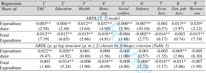
Results from the two models, for the expenditure variables of interest, are compared in Table 4.

The key differences between the two specifications, in terms of the expenditure share parameter estimates, are as follows. Firstly, the two expenditures previously found to have significant effects on GDP − T&C and education − have smaller parameter estimates in Table 4 but still statistically significant (at the 5% level). Secondly parameters for the other major spending shares of health, housing, social welfare and defence− are generally larger (in

27 _{Standard errors for long-run PMG parameters were obtained by the delta method.}

28 _{Pesaran and Shin (1999) argue from Monte Carlo experiments on the ARDL(p, m) model that the Schwarz Criterion}

is slightly superior to the Akaike Information Criterion.

29 _{Testing more than two lags is inhibited by the loss of degrees of freedom in our case.}

For Peer Review

absolute value) in Table 4 and are now statistically different from zero; negative in the case of social welfare and defence.30

[Table 4 about here]

Our interpretation of these results is that allowing the model to select the appropriate lag length is preferable. However, including additional lags by imposing two lags for all variables accommodates the possibility that the Schwarz Criterion eliminates some relevant lags. Imposing two-lags tends to strengthen, rather than weaken, the case for significant causal

effects from a number of public expenditure categories on long-run per capita GDP levels.

Weak exogeneity tests

As noted earlier, Pesaran and Shin (1999) contend that the PMG overcomes endogeneity, assuming zero cross-correlation among lagged errors. We address this by checking whether our fiscal variables are ‘weakly exogenous’ or ‘long-run forcing’ for the cointegrating parameters. Specifically, we test whether changes in the fiscal variables are statistically unrelated to the error correction term from the Table 3 regressions. Each fiscal variable may still react to its own lagged changes, lagged changes of other variables, or lagged changes in GDP growth. Based on Johansen (1992) and Boswijk (1995), we can test for weak exogeneity by estimating marginal models for each of our fiscal variables, using a variable addition test to assess the statistical significance of the error correction terms obtained from Table 3 regressions for each of those models. If the fiscal variables are confirmed as weakly exogenous, results in Tables 1 and 3 may be interpreted as causal effects.

Following Calderón et al. (2015), we test the following marginal models:

∆", = ,∆#, + ,∆#, + ,∆$, + ,∆$, + %&,' + , (4)

where ", represents each element of the vector Xi,t; &,' = $, − '#, are the

estimated long-run equilibrium error correction (ECM) terms, and εi,t is a random error term.31

Hence _Xi,t includes total expenditure, distortionary and non-distortionary taxes, non-residential

private investment (all as percentages of GDP), and the shares of each expenditure component in total public expenditure. The null hypothesis of weak exogeneity involves testing δi = 0, as a

t-test on the δi for each variable, or as a Wald test that the δis for all suspected endogenous

variables are jointly zero. Rejection of the null implies rejection of weak exogeneity.

For each of the nine estimations in Table 3, we estimate five different marginal models (for the four fiscal variables and investment) country by country. Like Calderón et al. (2015), we

use the MG approach to average the coefficients on the ECM term across countries and then

30 _{The smaller spending categories (general public, and recreation, services) appear non-robust, involving a change}

of sign.

31 _{Results reported below from regressions on (4) also include a constant term.}

For Peer Review

test its significance across the panel countries as a whole using the MG standard error. We also perform the equivalent weak exogeneity test for each country separately.

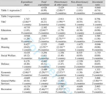
Row 1 of Table 5 shows results for weak exogeneity tests on the three fiscal variables and investment entering Table 1 regression (2) – the equivalent regression to those reported in Table 3 but excluding any expenditure share variables. Each cell contains the estimated t-ratio

for the unweighted average MG error correction parameters for each country. Beneath these values, the cell indicates the number of individual countries for which the null hypothesis of weak exogeneity is rejected. It can be seen that, for three of the four fiscal/investment variables we cannot reject weak exogeneity across the sample of countries. While the null hypothesis is rejected across all countries combined for one variable, ‘distortionary and other taxes’, it is clear that for all four variables in row 1, the null hypothesis is not rejected in all, or nearly all, countries. Hence one or two countries appear to drive the overall result for distortionary taxes.

[Table 5 about here]

Rows 2-10 show weak exogeneity test results for each expenditure share in Table 3. Of particular interest here is the t-ratio on each expenditure share variable (column 1). This reveals

that, only in the case of the T&C and economic services share is the mean MG parameter in the marginal model statistically significantly different from zero (at 5%). More importantly perhaps, across the 9 expenditure shares there is typically only 1 or 2 of the 17 countries for which the individual country value of δi is statistically non-zero. These results offer fairly

strong support to the view that the expenditure share variables can be considered weakly exogenous allowing us to interpret the estimated long-run expenditure parameters as capturing causal effects on GDP.

A similar conclusion emerges from Table 5 for the other variables in the regression. That is, the average MG parameter (across all countries) is not significantly different from zero in most cases, and this is also true for the vast majority of individual country estimates. Out of a total of 36 parameter sets (9 spending shares x 4 variables) for 17 countries, weak exogeneity is

never rejected in more than 4 out of 17 countries, is rejected for 3 or 4 out of 17 countries only 8 times (out of a possible 36), with the remainder rejected in only 0−2 out of the 17 countries.

Finally, the parameter ' in (4) which we have subjected to the weak exogeneity test is obtained from the previous model in which lag lengths were selected endogenously using the Schwarz Criterion, as described above. Given some uncertainty regarding the number of lags required to remove potential endogeneity, we re-ran Table 1 and Table 3 regressions on equation (3) imposing an ARDL (2, 2) structure. Weak exogeneity tests on these ' estimates are reported in the online appendix. If anything, they reveal even stronger support for weak exogeneity.

For Peer Review

From results in the previous sub-section we are inclined to be circumspect and, based on Table 3, claim evidence of exogenous positive impacts on GDP from changes in transport & communications and education spending. However, there is some, more limited support for positive (negative) effects on GDP from reallocating spending towards health and housing (social welfare and defence).

Short run dynamics

As the short run dynamics in the PMG regressions are allowed to differ across countries, it is possible that the short run output effects of a given fiscal change differ across countries both in initial direction and in the speed with which the long-run effect is realised. The trajectory followed by each country is determined by the estimated lag structure on each fiscal variable for that country together with its error-correction parameter.

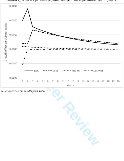
Given the noise associated with estimates of the short run dynamics for each country, little reliance can be placed on these estimates and we do not discuss them here.32 _{Instead, Figure 1} shows the average time path of GDP per capita growth rates associated with a 1 percentage point change in year 0 in each of the larger expenditure categories: T&C, education, health, and social security, based on Tables 3 regressions. We use the average of the country short run PMG parameters; hence obtained under the assumption of homogeneous long-run parameters which, for health and social welfare, are not statistically different from zero.

[Figure 1 about here]

As expected the figure suggests that GDP per capita growth converges on zero, as the level

of GDP per capita converges on its new long-run value following the 1% ‘shock’. However for the two significantly positive spending types (T&C, education) there is considerable persistence with effects on growth rates still evident after 20 years. In addition, the immediate impact (in years 1-2) is noticeably more positive for T&C than for education – a result that seems plausible given the known immediate output effects of infrastructure-related investment compared to education spending which can be expected to take longer to affect output. For social security, Figure 1 suggests the possibility of negative short run growth effects – also a plausible result as spending is reallocated from categories likely to be less dominated by transfers spending.

V. Conclusions

This paper has offered new evidence for OECD countries on the impact of the size and composition of public expenditure on per capita GDP. Previous regression analyses have been

32 _{In addition, Pesaran and Shin (1999, pp.372, 384-5) warn that, even though the long-run parameters obtained}

from the PMG are consistent and converge to their asymptotic values relatively quickly, short-run parameters converge more slowly. They also conclude that consistent estimation of short-run parameters requires explicit modelling of the contemporaneous dependence among the error terms of equations (2.1) and (2.2).

For Peer Review

unclear about which specific elements of the government budget are omitted from their analyses, or interpretation of parameter estimates is made difficult where several elements are explicitly or implicitly omitted. Clearly however, the method of financing any spending increase matters, whether this involves higher taxes (with differing distortionary characteristics), higher deficits, or reductions in alternative spending categories. Previous studies have also generally tested endogenous growth model specifications with permanent

growth effects, and endogeneity concerns remain regarding the reliability of these estimates.

Our examination of the impact of public expenditure on GDP for OECD countries has sought to deal explicitly with the financing aspects, allowed output growth effects to be persistent rather than permanent, and specifically addressed potential endogeneity concerns. Using longer time-series data than has been examined hitherto allowed us to apply more flexible (pooled mean group) methods that can accommodate heterogeneous short run responses across countries. We examined the GDP impacts of changes in total government expenditure, alongside changes in the shares of spending devoted to various categories.

Both our initial PMG results, and those that explicitly account for contemporaneous correlation, find robust long-run positive effects on per capita GDP levels for transport & communication and education, with some evidence supporting positive (negative) effects for housing and health (social welfare) spending. Results do not support positive long-run output effects from switching expenditure towards defense spending (sometimes claimed to have growth benefits). In our estimates, this switch involves pro-rata reductions in other spending.

Though our growth model specification precludes permanent effects on the growth rate of

per capita GDP, we nevertheless estimate relatively persistent effects on growth rates from simulated T&C and education expenditure changes that last for 20 years or more. Our results also confirm that the assumed form of expenditure financing is crucial and we find evidence of negative long-run effects on output from deficit-financed increases in total public spending. Our interpretation is that such spending increases cannot be expected to be growth-enhancing unless the specific forms of that expenditure are considered carefully.

The evidence of positive long-run effects on GDP per capita from increases in transport & communications, and education, spending shares appear to be robust and are consistent with

the message from an increasing body of recent research. This points to the possibility that current levels of such spending in OECD countries are sub-optimal from a growth perspective, though clearly this may be consistent with a wider social welfare objective.