Evolutionary Undersampling for Extremely Imbalanced Big Data
Classification under Apache Spark
I. Triguero, M. Galar, D. Merino, J. Maillo, H. Bustince, F. Herrera
Abstract— The classification of datasets with a skewed class distribution is an important problem in data mining. Evolu-tionary undersampling of the majority class has proved to be a successful approach to tackle this issue. Such a challenging task may become even more difficult when the number of the majority class examples is very big. In this scenario, the use of the evolutionary model becomes unpractical due to the memory and time constrictions. The divide-and-conquer approaches based on MapReduce paradigm have already been proposed to handle these types of problems by dividing data into multiple subsets. However, in extremely imbalanced cases, these models may suffer from a lack of density from the minority class in the subsets considered. Aiming at addressing this problem, in this contribution we provide a new big data scheme based on the new emerging technology Apache Spark to tackle highly imbalanced datasets. We take advantage of its in-memory operations to diminish the effect of the small sample size. The key point of this proposal lies on the independent management of majority and minority class examples, allowing us to keep a higher number of minority class examples in each subset. In our experiments we analyze the proposed model with several data sets with up to 17 million instances. The results show the goodness of this evolutionary undersampling model for extremely imbalanced big data classification.
I. INTRODUCTION
In the recent years, the amount of information that can be automatically gathered is inexorably growing in multiple fields such as bioinformatics, social media or physics. Thus, new class of data mining techniques that can take advantage of this voluminous data to extract valuable knowledge are required. This research topic is referred to under the term: big data [1]. Big data learning poses a significant challenge to the research community because standard data mining models cannot deal with the volume, diversity and complexity that these data bring up [2]. However, the newly arisen cloud platforms and parallelization technologies provide one with a perfect environment to tackle this issue.
The MapReduce framework [3], and its open-source im-plementation in Hadoop [4], were the first alternatives to
This work was supported by the Research Projects TIN2011-28488, TIN2013-40765-P, P10-TIC-6858 and P11-TIC-7765. I. Triguero holds a BOF postdoctoral fellowship from the Ghent University.
I. Triguero is with the Department of Internal Medicine of the Ghent
University, 9052 Zwijnaarde, Belgium. E-mails: {
D. Merino, J. Maillo and F. Herrera are with the Department of Computer Science and Artificial Intelligence of the University of Granada,
CITIC-UGR, Granada, Spain, 18071. E-mails: [email protected],{jesusmh,
herrera}@decsai.ugr.es
M. Galar and H. Bustince are with the Department of Automatics and Computation, Universidad P´ublica de Navarra, Campus Arrosad´ıa s/n, 31006
Pamplona, Spain. E-mails:{mikel.galar, bustince}@unavarra.es
handle data-intensive applications, which rely on a dis-tributed file system. The development of Hadoop-based data mining techniques has been widely spread [5], [6], because of its fault-tolerant mechanism (recommendable for time-consuming tasks) and its ease of use [7]. Despite its pop-ularity, researchers have encountered multiple limitations in Hadoop MapReduce to develop scalable machine learning tools [8]. Hadoop MapReduce is inefficient for applications that share data across multiple phases of the algorithms behind them, including iterative algorithms or interactive queries. Several platforms have recently emerged to over-come the issues presented by Hadoop MapReduce [9], [10]. Apache Spark [11] highlights as one of the most flexible and powerful engines to perform faster distributed computing in big data by using in-memory primitives. This platform allows us to load data into memory and query it repeatedly, making it very suitable for algorithms that use data iteratively.
The class imbalance problem is challenging when it appears in data mining tasks such as classification [12]. Focusing on two-class problems, the issue is that the positive instances are usually outnumbered by the negative ones, even though the positive one is usually the class of interest [13]. This problem is presented in a large number of real-world problems [12]. Furthermore, it comes along with a series of difficulties such as small sample size, overlapping or small disjuncts [14]. In this scenario, one focuses on correctly identifying the positive examples, but affecting the least to the negative class identification. Various solutions have been developed to address this problem, which can be divided into three groups: data sampling, algorithmic modifications and cost-sensitive solutions. These approaches have been success-fully combined with ensemble learning algorithms [15].
of the problem.
In [17], we proposed a MapReduce-based EUS scheme to tackle imbalance big data problems. This model splits the dataset into multiple chunks that are processed in different nodes (mappers) in such a way that EUS can be applied concurrently. Even though this model can scale to very large datasets, it may suffer from the small sample size problem. Within this divide-and-conquer procedure, a high number of maps implies having a considerably smaller amount of minority class examples in each one, what amplifies the lack of density problem.
In this work, we propose a big data scheme for ex-tremely imbalance problems implemented under Apache Spark, which aims at solving the lack of density problem in our previous model. We aim to exploit the flexibility provided by Spark, using other in-memory operations that alleviate the consumption costs of existing MapReduce alternatives. Multiple parallel operations compose the proposed frame-work. First, the whole training dataset is split into chunks, and the positive examples are extracted from it. Then, we broadcast the positive set, so that, all the nodes have a single in-memory copy of the positive samples. For each chunk of the negative data, we aim to obtain a balanced subset of data using a sample of the positive set. Later, EUS is applied to reduce the size of both classes and maximize the classification performance, obtaining a reduced set that is used to learn a model. Finally, the different models are combined to predict the classes of the test set. The source code of this model as well as the ones used in the experiments of this work are available at GitHub1.
The paper is structured as follows. Section II provides background information about imbalanced classification, EUS and MapReduce. Section III describes the proposal. Section IV analyzes the empirical results. Finally, Section V summarizes the conclusions.
II. BACKGROUND
This section briefly describes the topics used in this paper. First, the MapReduce paradigm and the Spark framework are introduced in Section II-A. Then, the state-of-the-art on imbalanced big data classification is presented (Section II-B), and the EUS algorithm is recalled (Section II-C).
A. MapReduce and Hadoop/Spark Frameworks
The MapReduce programming paradigm [3] is a scalable data processing tool designed by Google in 2003. It was designed to be part of the most powerful search-engine on the Internet, but it rapidly became one of the most effective techniques for general-purpose data intensive applications.
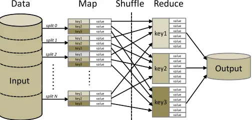
MapReduce is based on two user-defined operations: Map and Reduce. The Map function reads the raw data as key-value pairs <key,value>, and transforms them into a set of intermediate <key’,value’> pairs. Both key and value types are defined by the user. Then, MapReduce gener-ates multiple lists with all the values with the same key
1https://github.com/triguero/EUS-BigData
[image:2.612.313.565.125.245.2]<key’,list(value’)>(shuffle phase). Finally, the Reduce func-tion takes the grouped output from the maps and aggregates it into a smaller set of pairs<key”,value”>. Figure 1 shows a flowchart of MapReduce.
Fig. 1: Data flow overview of MapReduce
Apache Hadoop [18] is the most popular open-source implementation of MapReduce. It is widely used because of its performance, open source nature, installation facilities and its distributed file system (Hadoop Distributed File System, HDFS). Despite its popularity, Hadoop and MapReduce cannot deal with online or iterative computing, producing significant computational costs to reuse the data.
Apache Spark is a novel solution large-scale data process-ing to solve the drawbacks of Hadoop. Spark is part of the Hadoop Ecosystem and it uses the HDFS. This framework proposes a set of in-memory primitives, beyond the stan-dard MapReduce, aiming at processing data more rapidly on distributed environments. Spark is based on Resilient Distributed Datasets (RDDs), a special type of data structure used to parallelize the computations in a transparent way. These parallel structures let us persist and reuse results efficiently, since they are cached in memory. Moreover, they also let us manage the partitioning to optimize data placement, and manipulate data using transparent primitives.
B. Imbalanced classification in the Big Data context
A two-class classification dataset is imbalanced when it contains more instances from one class than from the other one. How to measure the performance of classification algorithms is a key issue in this framework, where the accuracy rate (percentage of correctly classified examples) is no longer valid. The most commonly considered alternatives in this scenario are the Area Under the ROC Curve (AUC) and the g-mean. The AUC (Area Under the ROC-Curve) [19] provides a scalar measurement of how well a classifier can trade off its true positive (TPrate) and false positive rates
(FPrate). A popular approximation [12] of this measure is
given by
AU C= 1 + TPrate−FPrate
2 . (1)
negative rates (TNrate) obtained by the classifier:
g-mean =pTPrate·TNrate (2)
The interest of this measure resides in the fact that equal weights are assigned to the classification accuracy over both classes. Both measures are interchangeably and extensively used in numerous experimental studies with imbalanced datasets [12], [16].
Big data solutions for classification problems can be affected by the presence of class imbalance. They can even worsen the problem if they are not properly designed. For example, an imbalanced dataset distributed across different nodes will maintain the imbalance ratio in each one, but it will have an even lower sample size due to the original division procedure. As a result, data subsets will be more affected by the small sample size problem than the original one, which is known to hinder classifier learning [12]. Therefore, meaningless classifiers can be learned in each node if they are treated independently without taking this issue into account first.
In [20], a set of data level algorithms to address im-balanced big data classification where tested (random un-der/oversampling and SMOTE). After applying these pre-processing mechanisms the Random Forest classifier [23] was applied. In other respects, the authors of [24] developed a fuzzy rule based classification system to deal with the class imbalance problem in a big data scenario adding a cost-sensitive model to the MapReduce adaptation of the algorithm. In [17], a preliminary approach to make EUS work in a big data setting was developed following a two-level parallelization model. As we have already mentioned, the greatest problem of this model was the small-sample size of the minority class, whose management with Hadoop framework was not fully automatic.
C. Evolutionary Undersampling
EUS [16] was developed as an extension of evolutionary prototype selection algorithms with special attention at the class imbalance problem [26]. In the case of EUS, the original objective of reducing the training set for the k -Nearest Neighbors (kNN) slightly changes, giving more focus to the balancing of the dataset and to the correct iden-tification of both classes of the problem in the subsequently used classifier. In order to obtain this new data subset, the instances of original dataset are encoded in a chromosome, which is evolved from randomly undersampled datasets until the best solution found cannot be further improved. The improvement is measured in terms of the fitness function, which in described afterwards.
In EUS, a binary chromosome is used to encode each possible solution. In the chromosome each bit represents the presence (1) or absence (0) of an instance in the training set. The search space is reduced by only considering the majority class instances for removal, including always all the minority class instances in the final dataset.
In order to rank the quality of the chromosomes a fitness function taking into account the balancing of the dataset and
the expected performance of the selected instances is used. The performance is estimated by the leave-one-out technique using the 1NN classifier and is measured by the g-mean (defined in Eq. (2)). The complete fitness function is as follows:
fitnessEUS = (
g-mean− 1−
n+ N− ·P
ifN
−>0
g-mean−P ifN−= 0,
(3)
where n+ is the number of positive instances, N− is the number of selected negative instances andP is a penalization factor that focuses on the balance between both classes.P is set to 0.2as recommended by the authors, since it provides a good trade-off between both objectives.
As a search algorithm, the CHC evolutionary algorithm [27] is chosen due to its excellent balance between explo-ration and exploitation. CHC is an elitist genetic algorithm making use of the heterogeneous uniform cross-over (HUX) for the combination of two chromosomes. It also considers an incest prevention mechanism and instead of applying mutation, it carries out a reinitialization of the population when the evolution does not progress.
III. EUS-EXTIMBBD: EVOLUTIONARY UNDERSAMPLING FOR EXTREMELY IMBALANCED BIG DATA
In this section we describe the proposed scheme for EUS of extremely imbalanced big data. First, we motivate our proposal in Section III-A, stating the main drawbacks of our previously proposed scheme. Then, Section III give the details of the proposed model.
A. Motivation
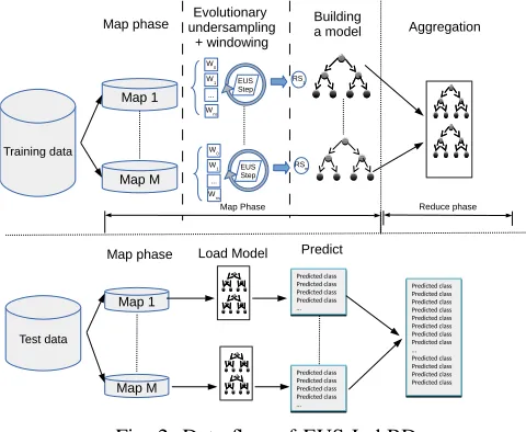
process was applied to classify the test set with the previously learned models. Figure 2 presents a flowchart of this model. In what follows, we denote this scheme as Evolutionary Undersampling for Imbalanced Big Data (EUS-ImbBD).
Fig. 2: Data flow of EUS-ImbBD.
This model suffers of two main drawbacks that motivates this work:
• Although EUS-ImbBD can handle very large datasets with the appropriate number of nodes, it may experience troubles to tackle extremely imbalanced problems in which the imbalance ratio is very high. In these cases, the amount of positive examples in the different chunks of the data created by the MapReduce process may not be sufficient (or even null) to guide an EUS process. This problem is known as the small sample size or lack of density problem. This is the main point motivating our works, since EUS-ImbBD becomes not totally scal-able in this scenario.
• EUS-ImbBD requires to concatenate two MapReduce
phases, to build a model and to classify a test set, respectively. Hadoop is inefficient with these types of models, whereas Spark allows us to avoid the startup costs. In Section IV the differences between Hadoop and Spark implementations of this scheme can be observed. The aim of this paper is tackle both issues by designing an imbalance big data model, which relies on the flexibility an in-memory operations of Apache Spark.
B. EUS-S-ExtImbBD: A Spark-based Design of Evolutionary Undersampling for Extremely Imbalanced Big Data
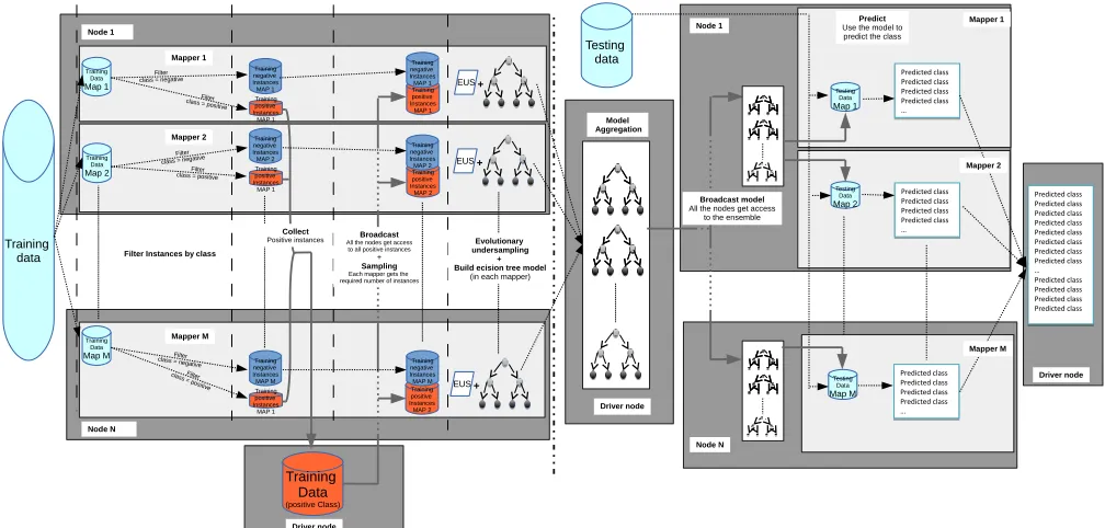
This section introduces the proposed scheme in terms of multiple Spark distributed operations. Algorithm 1 shows the pseudo-code of the whole method with precise details of the functions utilized from Spark and Figure 3 summarizes the data flow of the algorithm. In the following, we describe the most significant instructions, enumerated from 1 to 12.
Let trainFile be the training set stored in the HDFS as a single file. This file is formed of h HDFS blocks that
Algorithm 1 EUS-S-ExtImbBD
Require: trainFile; testFile; #Maps; {Building Phase}
1:trainRDD←textFile(trainFile, #Maps).cache()
2:posTrainRDD = trainRDD.filter(line→line.contains(”positive”)).collect()
3:negTrainRDD = trainRDD.filter(line→line.contains(”negative”))
4:posTrainBroadcast = broadcast(posTrainRDD)
5:models←negTrainRDD.mapPartitions(negTrainPartition→
createModel(negTrainPartition, posTrainBroadcast.value)).collect() {Classification Phase}
6:testRDD←textFile(testFile)
7:modelsBroadcast = broadcast(models)
8:classification = testRDD.mapPartitions( testPartition→
classify(testPartition, modelsBroadcast) )
9:confMatrix←calculateConfusionMatrix(classification.toArray)
10: (AUC, GM)←computePerformance(confMatrix)
can be accessed from any computer. The building phase starts reading the whole trainFile set from HDFS as an RDD, splitting the dataset into an user-defined number of #Mapdisjoint subsets (Instruction 1). This operation spreads the data across the computing nodes, caching the different subsets (Map1,Map2,...,Mapm) into memory.
Next, we split this dataset into two subsets: positive set posTrainRDDand negative setnegTrainRDD, which contain only positive and negative instances, respectively. The filter transformation provided by Spark is used for this purpose (Instructions 2 and 3).
Assuming that the number of positive instances fit in-memory, the wholeposTrainRDDis collected and broadcast to all the computing nodes (Instruction 4). The broadcast function of Spark allows us to keep a read-only variable cached on the main memory of each machine rather than copying it with each tasks. Note that this can be a limitation of the current model, since if the number of positive instances is too high it may not fit in memory. However, this set of instances is stored only once in each node independently of the number of tasks executed in it. In the current real-world problems we are facing, with an extremely high imbalance ratios, this situation is difficult to be found. Anyway, in the future our aim is to further investigate problems with this scenario even though they may not suffer from the small-sample size problem due to the fact that more positive instances are available.
After that, the main map phase starts over the #M ap
partitions (negTrainPartition) of negative set negTrainRDD (Instruction 5). ThemapPartitions(func)transformation runs the function defined in Algorithm 2 on each block of the RDD concurrently. This function builds a model from the available data, i.e., a subset of negTrainPartition, and the whole posTrainBroadcast set. Depending on the dataset at hand, we may encounter two different situations:
Node N Driver node Node 1 Mapper 1 Mapper 2 Driver node Training positive Instances MAP 2 Training positive Instances MAP 2 Training data EUS
Filter Instances by class Training Data Map 2 Training Data Map 1 Training Data Map M Training negative Instances MAP 1 Training negative Instances MAP 2 Training negative Instances MAP M Training positive Instances MAP 1 Training positive Instances MAP 1 Training positive Instances MAP 1 Training Data (positive Class) Broadcast All the nodes get access to all positive instances
+ Sampling Each mapper gets the required number of instances
Training negative Instances MAP 2 Training negative Instances MAP M Filter
class = negative
Filter class = positive
Filter class =
positive Filter class = positive
Filter class = negative
Filter class = negative
Training positive Instances MAP 1 Training negative Instances MAP 1 Collect Positive instances Model Aggregation + Evolutionary undersampling + Build ecision tree model
(in each mapper)
EUS+ EUS+ Mapper M Driver node Testing data Testing Data Map 2 Testing Data Map 1 Testing Data Map M Broadcast model All the nodes get access
to the ensemble
Predicted class Predicted class Predicted class Predicted class … Predicted class Predicted class Predicted class Predicted class … Predicted class Predicted class Predicted class Predicted class … Predicted class Predicted class Predicted class Predicted class … Predicted class Predicted class Predicted class Predicted class Predicted class Predicted class Predicted class Predicted class … Predicted class Predicted class Predicted class Predicted class Predicted class Predicted class Predicted class Predicted class Predicted class Predicted class Predicted class Predicted class … Predicted class Predicted class Predicted class Predicted class Predict
Use the model to predict the class
[image:5.612.52.556.55.296.2]Predicted class Predicted class Predicted class Predicted class … Predicted class Predicted class Predicted class Predicted class … Node 1 Node N Mapper 1 Mapper 2 Mapper M
Fig. 3: Data flow of EUS-ExtImbBD.
if the problem is almost balanced (IR <= 1.5 as suggested in the literature), instances from both classes are considered in the selection procedure, since the balancing looses importance in favor of an appropriate interaction between the instances of both classes (always maintaining a balance between their presence).
• When we the size of the positive class is larger than that of the negative one, we make use of a random subset of positive instances posTrainSubset from the whole positive set posTrain. Our aim is to balance the class distribution before applying EUS to reduce the size of both classes while focusing on maintaining a balance and obtaining the best performance as possible.
Algorithm 2 CreateModel function
Require: negTrainPartition, posTrain{posTrain comes from the broadcast variable}
1: ifposTrain.size()<negTrainPartition.size() then
2: trainingSet = posTrain∪negTrainPartition
3: else
4: posTrainSubset←takeRandomSubset(posTrain, negTrainPartition.size() )
5: trainingSet←posTrainSubset∪negTrainPartition
6: end if
7: reducedTrainSet←EUS windowing(trainingSet)
8: model←buildModel(reducedTrainSet)
9: return model
In both cases, EUS is applied with the windowing scheme. We refer the reader to [17] for more details on this respect. At the end of the EUS stage, a reduced and balanced set of instances (reducedTrainSet) is obtained. Then, the learning phase is carried out, which consists of building a decision tree. More specifically, we consider the well-known C4.5 algorithm [29] for its great behavior in classifier ensembles. As a result of the map phase, we obtain #M apdecision trees that are returned to the driver and collected in Instruc-tion 5 of Algorithm 1.
Then, the classification step estimates the class associated to each test example. Given that in big data problems the test set can also be very large, we assume this set is also stored in the HDFS as a single file (testFile), and read it as an RDD (Instruction 6). In order to classify the instances in each block, the models are broadcast to the main memory of all the computing nodes of the cluster (Instruction 7). A new map operation will tackle each subset of the test set. Algorithm 3 summarizes the operations that are carried out. Basically, the predictions in each block are estimated by the majority vote of the all the decision trees built in the previous phase (Instruction 8). Finally, the classification performed is collected in the driver and the performance measures are computed (Instructions 9 and 10).
Algorithm 3 Classify
Require: testPartition, models
1:testPartitionPredictions←testPartition.foreach{
instance→majority(models.foreach{model→model.classify(instance)})}
{majority takes and array of predicted classes and returns the most repeated one} 2:return testPartitionPredictions
As a final remark, note that the EUS algorithm could be easily replaced by other data sampling approaches, without changing the general framework we propose in here.
IV. EXPERIMENTAL STUDY
This section establishes the experimental setup (Section IV-A) and discusses the results obtained (Section IV-B.2).
A. Experimental Framework
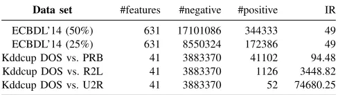
Competition ECBDL’14 [30], [6]. For this study, we consider two subsets of 25% and 50% of the instances, respectively. The second dataset corresponds to the KDD Cup 1999 data set, available in the UCI machine learning repository [31]. Since it contains multiple classes, we have formed several case studies from them, obtaining as a result two-class im-balanced problems. Specifically, we have taken the majority class (i.e., DOS) in comparison with the rest of the minority classes (i.e., PRB, R2L and U2R) in order to investigate the influence of different IRs. The data characteristics are summarized in Table I.
TABLE I: Data sets considered for the experimental study.
Data set #features #negative #positive IR
ECBDL’14 (50%) 631 17101086 344333 49
ECBDL’14 (25%) 631 8550324 172386 49
Kddcup DOS vs. PRB 41 3883370 41102 94.48
Kddcup DOS vs. R2L 41 3883370 1126 3448.82
Kddcup DOS vs. U2R 41 3883370 52 74680.25
In this study, independently of the technology (Hadoop or Spark) used, we distinguish between two different ap-proaches to tackle imbalanced big data classification:
• EUS-ImbBD: EUS for Imbalanced Big Data, i.e., the model presented in [17], which consists of dividing the training set in a single MapReduce operation.
• EUS-ExtImbBD: EUS of Extremely Imbalanced Big Data problems, i.e., the scheme presented in this work, which considers the positive and negative training ex-amples separately.
Originally, EUS-ImbBD was implemented under Hadoop (EUS-H-ImbBD), whereas EUS-ExtImbBD has been de-signed for Spark (EUS-S-ExtImbBD). However, in order to be able to perform a comparison between Hadoop and Spark technologies, we have implemented these models in both technologies, naming them as H-ExtImbBD and EUS-S-ImbBD, respectively. The comparison between Hadoop and Spark implementations will be done using KDD Cup dataset, as this was the one considered in the original work. Note that the application of EUS-ExtImbBD within Hadoop, one must manually pre-partition the training dataset into positive and negative sets, and the MapReduce stage is applied simply over the negative set, as it was done in [17], whereas the positive set has to be read in all the tasks (even if they are in the same node).
In addition to these models, we have implemented RUS in Spark under the original ImbBD scheme as a comparison algorithm, calling it RUS-S-ImbBD. Since RUS objective is to randomly balance the dataset eliminating negative class examples, this can be done in each mapper regardless of the number of instances from both classes in it, and hence it is not necessary to apply it under the scheme proposed for extremely imbalance data.
It is important to note that for the last two data sets presented in Table I, we have so few positive examples
[image:6.612.53.297.220.289.2]that the ImbBD approach cannot be applied, and EUS-ExtImbBD is required.
TABLE II: Parameter settings for the used methods.
Method Parameter values
EUS-ImbBD[17] MapReduce Building: Number Of Maps = 128/256/512; Number Of Reducers:1 Windowing in Majority Class = Imbalanced Ratio
MapReduce Classification: Number Of Maps = Same as Building phase; Number Of Reducers:0
EUS-ExtImbBD Building phase: Number Of Maps = 128/256/512/1024/2048; Windowing in majority class= IR; Windowing in both classes = 5 Classification phase: Number Of Maps = Same as Building phase;
RUS-S-ImbBD Building phase: Number Of Maps = 1024/2048;
Classification phase: Number Of Maps = Same as Building phase;
In our experiments we consider a 5-fold stratified cross-validation model, meaning that we construct 5 random par-titions of each dataset maintaining the prior probabilities of each class. Each fold, corresponding to 20% of the data is used once as test set, evaluated on a model trained on the combination of the 4 remaining folds. The reported results are taken as averages of the five partitions. To evaluate our model, we consider the AUC and g-mean measures recalled in Section II-B. Moreover, we evaluate the time requirements of the methods in two ways:
• Building time: we will quantify the total time in seconds spent by our method to generate the resulting learned model.
• Classification time: this refers to the time needed in seconds to classify all the instances of the test set with the given learned model.
We will also investigate how these measures are affected by modifying the number of maps. The experiments have been carried out on twelve nodes in a cluster: a master node and eleven computing nodes. Each one of these computing nodes has 2 Intel Xeon CPU E5-2620 processors, 6 cores per processor (12 threads), 2.0 GHz and 64GB of RAM. The network is Gigabit ethernet (1Gbps). In terms of software, we have used the Cloudera’s open-source Apache Hadoop distribution (Hadoop 2.6.0-cdh5.4.2) and Spark 1.5.1. A maximum of 216 concurrent tasks are available.
B. Results and discussion
This section presents and analyzes the results obtained in the experimental study. We divide this section into two parts: Subsection IV-B.1 briefly compares Hadoop and Spark implementations, and Subsection IV-B.2 deeply analyzes the performance of the proposed approach in a larger problem.
1) Comparing Hadoop vs. Spark: The goal of this sub-section is to compare the Hadoop and Spark technologies in terms of efficiency, when they implement the same model. To do this, we focus on the three different variants of the Kddcup dataset. The EUS-ImbBD approach is used for DOS vs. PRB dataset, whereas EUS-ExtImbBD is applied in the other two Kddcup versions as explained before. Table III shows the runtime required in both building and classification phases, depending on the technology used, as well as the percentage of improvement obtained with Spark over Hadoop.
TABLE III: Running times obtained by the Hadoop and Spark implementations of EUS-ImbBD and EUS-ExtImbBD.
Hadoop-based Spark-based Spark improvement
Dataset No. of maps Build time (s) Classif. time (s) Build time(s) Classif. time (s) Build time Classif. time Kddcup DOS vs. PRB 128 422.4786 34.264 297.5048 0.2942 29.58% 99.14% 256 240.4662 36.7934 143.3428 0.3566 40.39% 99.03% 512 156.4354 48.424 87.0195 0.2739 44.37% 99.43% Kddcup DOS vs. R2L 128 444.7252 31.7255 320.8192 0.0876 27.86% 99.72% 256 266.2424 36.1147 187.4562 0.1024 29.59% 99.72% 512 178.8536 42.0057 148.319 0.1371 17.07% 99.67% Kddcup DOS vs. U2R 128 459.6002 31.8436 340.2297 0.0986 25.97% 99.69% 256 248.1038 35.5862 193.0784 0.1081 22.18% 99.70% 512 152.3752 46.6194 101.683 0.1275 33.27% 99.73%
• Even though the same EUS process has been applied
in both technologies, the Spark-based implementation has always reported a faster runtime in both building and classification phases. It is remarkable that applying EUS-ExtImbBD, Spark is still much faster, although the Hadoop version already started from two manually partitioned datasets (whose added cost is not included in the runtime). Moreover, it is specially significant the reduction in terms of classification, due to the startup costs of Hadoop MapReduce.
• From the flexibility point of view, Spark has allowed us to apply the whole procedure in a single program, while in Hadoop, multiple MapReduce programs needs to be chained. Hence, Spark is more versatile.
In conclusion the use of Spark has provided us a greater flexibility and efficiency. In the next experiments, we will only consider Spark to tackle larger datasets.
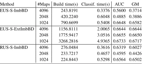
2) Analysis of the performance: To analyze the perfor-mance of the proposed EUS-S-ExtImbBD scheme, we focus on the ECBLD’14 dataset. Tables IV and V show the results obtained by our proposal in comparison to the previous al-ternative (EUS-S-ImbBD) and random undersampling (RUS-S-ImbBD) in ECBLD’14 (25%) and ECBLD’14 (50%), respectively. All of these techniques are implemented under Apache Spark for a faster computation. The averaged AUC, g-mean, building and classification runtime are presented, depending on the number of mappers used (#Maps).
TABLE IV: Results obtained in ECBLD’14 (25%)
Method #Maps Build time(s) Classif. time(s) AUC GM
EUS-S-ImbBD 4096 243.8191 0.3376 0.5600 0.3714
2048 420.2240 0.6048 0.4885 0.3886
1024 790.6699 0.5408 0.6648 0.6582
EUS-S-ExtImbBD 4096 1156.8111 2.0065 0.6644 0.6644
2048 1775.9417 3.0516 0.6655 0.6650
1024 3268.2816 4.9365 0.6733 0.6717
RUS-S-ImbBD 4096 276.0484 0.3616 0.6319 0.6027
2048 233.7217 0.4657 0.4595 0.4426
1024 224.8443 0.5298 0.6564 0.6502
From these tables we can highlight several factors:
[image:7.612.313.557.245.356.2]• When the number of maps is increased, we can observe
TABLE V: Results obtained in ECBLD’14 (50%)
Method #Maps Build time(s) Classif. time(s) AUC GM
EUS-S-ImbBD 8192 497.0958 0.4999 0.5556 0.3572
4096 775.2016 0.5531 0.4821 0.4276
2048 1476.3512 0.7878 0.6674 0.6645
EUS-S-ExtImbBD 8192 2181.5089 3.5404 0.6641 0.6640
4096 3456.5938 6.0428 0.6662 0.6657
2048 6433.8072 9.4064 0.6731 0.6704
RUS-S-ImbBD 8192 557.4869 0.5540 0.6319 0.6066
4096 518.1471 1.0960 0.4659 0.4339
2048 483.7361 1.0960 0.6651 0.6622
how the EUS-S-ImbBD scheme falls into the small sample size problem. The reduction of the number of positive examples in the different maps makes AUC and GM measures to drastically drop when more maps are required. AUC values are sometimes even lower than0.5meaning that an inappropriate model has been learned (worse than random guessing).
• On the other side, the proposed EUS-S-ExtImbBD has been able to avoid this issue by using a higher number positive examples in each map. We can observe how the decrease in precision when the number of maps is increased is much smoother in this case. Nevertheless, since EUS is dealing with a larger number of examples in each map in comparison with EUS-S-ImbBD, the total runtime required becomes higher for this proposal.
• Comparing with the application of a simple random
undersampling (RUS-S-ImbBD), we can observe that the capabilities of EUS are maintained and that it is able to outperform RUS in terms of precision. Of course, the time required by RUS is much lower, since it does not involve any heuristic mechanism to select elements from the negative class.
• Note that the number of concurrent tasks in the used cluster is 216. Thus, we cannot expect a linear speedup in the runtime required by RUS. We do appreciate a linear complexity reduction for EUS due to the quadratic complexity of this problem.
[image:7.612.55.298.585.696.2]attending at their instability when addressing the same problem with different number of mappers. Notice that after the sampling process a C4.5 decision tree is built, and not only its building process is affected by the number and class of the examples selected but also its pruning may vary (which can explain the instability of these models).
Attending at these results, one can conclude that the new EUS model for addressing extremely imbalanced problems with Spark overcome the problems of our previous alterna-tives. Moreover, the flexibility of Spark has allowed us to make a simple and fully automatic implementation of the proposed model.
V. CONCLUDING REMARKS
In this contribution we have devised a big data scheme to deal with the rare situation where data scarcity (of a partic-ular class) remains to be a problem despite the vast quantity of available data. The application of the proposed strategy enables EUS to be applied on big datasets with extremely skewed class distributions by an effective use of the avail-able data. Our implementation is based on multiple parallel operations and takes advantage of the in-memory operations provided by Apache Spark. Our experimental study shows the benefits of using Spark as parallelization technology and the advantages of our new framework to soften the lack of density issue presented in these extremely imbalanced problems. As future work, we consider the development of efficient big data strategies that can deploy preprocessing mechanisms such as hybrid oversampling/undersampling ap-proaches in the big data context. Regarding the proposed method, techniques to deal with extremely imbalanced prob-lems where the positive class does not fit in the main memory of the computing nodes will be studied.
REFERENCES
[1] C. Lynch, “Big data: How do your data grow?”Nature, vol. 455, no.
7209, pp. 28–29, 2008.
[2] M. Minelli, M. Chambers, and A. Dhiraj, Big Data, Big Analytics:
Emerging Business Intelligence and Analytic Trends for Today’s Busi-nesses (Wiley CIO), 1st ed. Wiley Publishing, 2013.
[3] J. Dean and S. Ghemawat, “Mapreduce: simplified data processing
on large clusters,”Communications of the ACM, vol. 51, no. 1, pp.
107–113, Jan. 2008.
[4] S. Ghemawat, H. Gobioff, and S.-T. Leung, “The google file system,” in Proceedings of the nineteenth ACM symposium on Operating systems principles, ser. SOSP ’03, 2003, pp. 29–43.
[5] A. Srinivasan, T. Faruquie, and S. Joshi, “Data and task parallelism in
ILP using mapreduce,”Machine Learning, vol. 86, no. 1, pp. 141–168,
2012.
[6] I. Triguero, S. del R´ıo, V. L´opez, J. Bacardit, J. M. Ben´ıtez, and F. Herrera, “ROSEFW-RF: The winner algorithm for the ecbdl’14 big data competition: An extremely imbalanced big data bioinformatics
problem,”Know.-Based Syst., vol. 87, no. C, pp. 69–79, Oct. 2015.
[7] A. Fern´andez, S. R´ıo, V. L´opez, A. Bawakid, M. del Jesus, J. Ben´ıtez, and F. Herrera, “Big data with cloud computing: An insight on the computing environment, mapreduce and programming frameworks,”
WIREs Data Mining and Knowledge Discovery, vol. 4, no. 5, pp. 380– 409, 2014.
[8] K. Grolinger, M. Hayes, W. Higashino, A. L’Heureux, D. Allison,
and M. Capretz, “Challenges for mapreduce in big data,” inServices
(SERVICES), 2014 IEEE World Congress on, June 2014, pp. 182–189.
[9] Y. Low, J. Gonzalez, A. Kyrola, D. Bickson, C. Guestrin, and J. M. Hellerstein, “Graphlab: A new parallel framework for machine
learn-ing,” inConference on Uncertainty in Artificial Intelligence (UAI),
Catalina Island, California, July 2010.
[10] Y. Bu, B. Howe, M. Balazinska, and M. D. Ernst, “Haloop: Efficient
iterative data processing on large clusters,”Proc. VLDB Endow., vol. 3,
no. 1-2, pp. 285–296, Sep. 2010.
[11] M. Zaharia, M. Chowdhury, T. Das, A. Dave, J. Ma, M. McCauley, M. J. Franklin, S. Shenker, and I. Stoica, “Resilient distributed datasets: A fault-tolerant abstraction for in-memory cluster
comput-ing,” in Proceedings of the 9th USENIX conference on Networked
Systems Design and Implementation. USENIX Association, 2012, pp. 1–14.
[12] V. L´opez, A. Fern´andez, S. Garc´ıa, V. Palade, and F. Herrera, “An insight into classification with imbalanced data: Empirical results and
current trends on using data intrinsic characteristics,” Information
Sciences, vol. 250, no. 0, pp. 113 – 141, 2013.
[13] G. Weiss, “Mining with rare cases,” inData Mining and Knowledge
Discovery Handbook. Springer, 2005, pp. 765–776.
[14] M. Galar, A. Fern´andez, E. Barrenechea, H. Bustince, and F. Herrera, “A review on ensembles for the class imbalance problem:
Bagging-, boosting-Bagging-, and hybrid-based approachesBagging-,” IEEE Transactions on
Systems, Man, and Cybernetics, Part C: Applications and Reviews, vol. 42, no. 4, pp. 463–484, 2012.
[15] M. Galar, A. Fern´andez, E. Barrenechea, and F. Herrera, “Eusboost: Enhancing ensembles for highly imbalanced data-sets by evolutionary
undersampling,”Pattern Recognition, vol. 46, no. 12, pp. 3460–3471,
2013.
[16] S. Garc´ıa and F. Herrera, “Evolutionary under-sampling for
classifica-tion with imbalanced data sets: Proposals and taxonomy,”Evolutionary
Computation, vol. 17, no. 3, pp. 275–306, 2009.
[17] I. Triguero, M. Galar, S. Vluymans, C. Cornelis, H. Bustince, F. Her-rera, and Y. Saeys, “Evolutionary undersampling for imbalanced big
data classification,” inEvolutionary Computation (CEC), 2015 IEEE
Congress on, May 2015, pp. 715–722.
[18] A. H. Project, “Apache hadoop,” 2013. [Online]. Available:
http://hadoop.apache.org/
[19] T. Fawcett, “An introduction to roc analysis,” Pattern recognition
letters, vol. 27, no. 8, pp. 861–874, 2006.
[20] S. del R´ıo, V. L´opez, J. Ben´ıtez, and F. Herrera, “On the use of
mapreduce for imbalanced big data using random forest,”Information
Sciences, vol. 285, pp. 112–137, 2014.
[21] G. Batista, R. Prati, and M. Monard, “A study of the behavior of
several methods for balancing machine learning training data,”ACM
Sigkdd Explorations Newsletter, vol. 6, no. 1, pp. 20–29, 2004. [22] N. Chawla, K. Bowyer, L. Hall, and W. Kegelmeyer, “SMOTE:
synthetic minority over-sampling technique,” arXiv preprint
arXiv:1106.1813, 2011.
[23] L. Breiman, “Random forests,”Machine learning, vol. 45, no. 1, pp.
5–32, 2001.
[24] V. L´opez, S. del R´ıo, J. Ben´ıtez, and F. Herrera, “Cost-sensitive linguistic fuzzy rule based classification systems under the mapreduce
framework for imbalanced big data,”Fuzzy Sets and Systems, vol. 258,
pp. 5–38, 2014.
[25] H. Ishibuchi, T. Nakashima, and M. Nii,Classification and modeling
with linguistic information granules. Springer, 2005.
[26] S. Garc´ıa, J. Derrac, J. Cano, and F. Herrera, “Prototype selection for
nearest neighbor classification: Taxonomy and empirical study,”IEEE
Transactions on Pattern Analysis and Machine Intelligence, vol. 34, no. 3, pp. 417–435, 2012.
[27] L. J. Eshelman, “The CHC adaptive search algorithm: How to have safe search when engaging in nontraditional genetic recombination,” inFoundations of Genetic Algorithms, G. J. E. Rawlins, Ed. San Francisco, CA: Morgan Kaufmann, 1991, pp. 265–283.
[28] I. Triguero, D. Peralta, J. Bacardit, S. Garcia, and F. Herrera, “A combined mapreduce-windowing two-level parallel scheme for
evo-lutionary prototype generation,” inEvolutionary Computation (CEC),
2014 IEEE Congress on, July 2014, pp. 3036–3043.
[29] J. R. Quinlan,C4.5: programs for machine learning. San Francisco,
CA, USA: Morgan Kaufmann Publishers, 1993.
[30] “ECBDL14 dataset: Protein structure prediction and contact map for the ECBDL2014 big data competition,” 2014. [Online]. Available: http://cruncher.ncl.ac.uk/bdcomp/