A learning automata based multiobjective hyper heuristic

For Peer Review

A Learning Automata based Multiobjective Hyper-heuristic

Journal: Transactions on Evolutionary Computation

Manuscript ID TEVC-00119-2017.R2

Manuscript Type: Regular Papers

Date Submitted by the Author: n/a

Complete List of Authors: Li, Wenwen; University of Nottingham, Computer Science School Özcan, Ender; University of Nottingham, Computer Science

John, Robert; University of Nottingham, School of Computer Science

Keywords: Online learning, Multiobjective optimisation, Hyper-heuristics, Evolutionary algorithms, Operational research

For Peer Review

A Learning Automata based Multiobjective

Hyper-heuristic

Wenwen Li, Ender ¨

Ozcan, and Robert John

Abstract—Metaheuristics, being tailored to each particular domain by experts, have been successfully applied to many computationally hard optimisation problems. However, once im-plemented, their application to a new problem domain or a slight change in the problem description would often require additional expert intervention. There is a growing number of studies on reusable cross-domain search methodologies, such as, selection hyper-heuristics, which are applicable to problem instances from various domains, requiring minimal expert intervention or even none. This study introduces a new learning automata based selection hyper-heuristic controlling a set of multiobjective metaheuristics. The approach operates above three well-known multiobjective evolutionary algorithms and mixes them, exploit-ing the strengths of each algorithm. The performance and be-haviour of two variants of the proposed selection hyper-heuristic, each utilising a different initialisation scheme are investigated across a range of unconstrained multiobjective mathematical benchmark functions from two different sets and the real-world problem of vehicle crashworthiness. The empirical results illustrate the effectiveness of our approach for cross-domain search, regardless of the initialisation scheme, on those problems when compared to each individual multiobjective algorithm. Moreover, both variants perform signicantly better than some previously proposed selection hyper-heuristics for multiobjective optimisation, thus signicantly enhancing the opportunities for improved multiobjective optimisation.

Index Terms—Online learning, Multiobjective optimisation, Hyper-heuristics, Evolutionary algorithms, Operational research

I. INTRODUCTION

Multiobjective optimisation problems (MOPs) require si-multaneous handling of various and often conflicting objec-tives during the search process. The solution methods designed for MOPs seek a set of ‘equivalent’ solutions, each reflecting atrade-off between different objectives.

There are distinct complexities associated with MOPs mak-ing the development of effective and efficient solution methods extremely challenging (e.g., very large search spaces, noise, uncertainty, etc.). Metaheuristics, in particular, multiobjective evolutionary algorithms (MOEAs) are the most commonly used search methods in the area of solving MOPs. One of the main advantages of MOEAs is that they are population based techniques, capable of obtaining a set of trade-off solutions with reasonable quality even in a single run [1]. Even though ‘optimality’ can not be guaranteed, empirical results indicate the success of MOEAs on a variety of problem domains, including planning and scheduling ([2], [3]), data mining [4],

W. Li, E. ¨Ozcan and R. John are with the ASAP research group, School of Computer Science, University of Nottingham, UK

E-mail:{psxwl8,pszeo,pszrij}@nottingham.ac.uk

and circuits and communications [5]. There are different types of MOEAs, each utilising different algorithmic components during the search process and so perform differently. In the majority of the previous studies, individual MOEAs are designed and applied to a particular problem in hand. More on MOEAs and their applications to various multiobjective problems can be found in [6].

On the other hand, there is a growing number of studies onselection hyper-heuristicswhich provide a general-purpose heuristic optimisation framework for utilising the strengths of multiple (meta)heuristics [7]. Selection hyper-heuristics con-trol and mix low level (meta)heuristics, automatically deciding which one(s) to apply to the candidate solution(s) at each decision point of the iterative search process [8]. Raising the generality level of heuristic optimisation methods is one of the main motivations behind the hyper-heuristic studies. The idea is, through automation of the heuristic search, to provide effective and reusable cross-domain search method-ologies which are applicable to the problems with different characteristics from various domains without requiring much expert involvement.

Learning is key to develop an effective selection hyper-heuristic with the adaptation capability. There are some recent studies looking into the interplay between data science tech-niques, particularly machine learning algorithms and selection hyper-heuristics leading to an improved overall performance. For example, [9] and [10] used tensor analysis as a machine learning approach to decide which low level heuristics to employ at different stages of the search process. In [11], the feasibility and effectiveness of using reinforcement learning to improve the performance of metaheuristics and hyper-heuristics have been discussed in depth. [12] introduced an effective multi-stage hyper-heuristic for cross-domain search which first, reduces the low level heuristics to be used in the following stage based on a multiobjective learning strategy and then mixes them under a stochastic local search frame-work. More recently, computational intelligence techniques have been used as components of general purpose methods managing low level (meta)heuristics for overall performance improvement. For example, [13] introduced a fuzzy inference selection based hyper-heuristic which mixed and controlled four search operators, each derived from a different meta-heuristic to solve a computationally hard problem of t-way test suite generation. However, the aforementioned studies all focus on single objective optimisation. There have been some studies on combining the strengths of multiple MOEAs with the aim of providing a better overall performance for multiobjective optimisation under a selection hyper-heuristic

For Peer Review

framework (e.g., [14], [15]). From this point onward, we will refer to such selection hyper-heuristics asmultiobjective hyper-heuristics (MOHHs).

In this study, we present a new learning automata based selection hyper-heuristic framework with implementation of two variants, Learning Automata based Hyper-heuristic (HH-LA) and Learning Automata based Hyper-heuristic with a Ranking Scheme Initialisation (HH-RILA) for multiobjective optimisation. Both selection hyper-heuristics mix and control a set of three well-known MOEAs: nondominated sorting ge-netic algorithm (NSGA-II) [16], strength Pareto evolutionary algorithm 2 (SPEA2) [17] and indicator based evolutionary algorithm (IBEA) [18]. The learning automaton acts as a guidance for choosing the appropriate MOEA at each de-cision point while solving a given problem. The proposed two variants of selection hyper-heuristics mainly differ in their initial set-up process. HH-LA employs all three low level MOEAs and gives an equal chance initially to each algorithm making a random start. HH-RILA applies a rank-ing scheme which eliminates the relatively poor performrank-ing MOEA(s) and uses the remaining MOEAs in the improvement process (Section III-A). The performance of the proposed hyper-heuristics are investigated against a variety of other multiobjective approaches across a range of multiobjective problems, including well-known benchmark functions and a real-world problem of vehicle crashworthiness. The empirical results indicate the effectiveness and generality of the proposed hyper-heuristics with novel components.

The rest of the paper is organised as follows. Section II introduces some essential concepts of MOPs, selection multiobjective hyper-heuristics as well as learning automata and provides background for vehicle crashworthiness. Section III presents the details of the proposed method which embeds three novel components. Firstly, the learning automaton com-ponent designed for multiobjective optimisation operates in a non-traditional way as explained in Section III-B. The second component, as described in Section III-C supports the develop-ment of a two-stage metaheuristic selection approach based on the information obtained from the learning process, enabling the use of two different metaheuristic selection methods at different stages. The third component as described in Section III-D adaptively decides when to switch to another MOEA depending on a tuned improvement threshold parameter. The parameter tuning and setting are included in Section IV, as well as the discussion and analysis of the experimental results. Section V concludes this study and provides directions for future work.

II. BACKGROUND

A. Related Work on Multiobjective Selection Hyper-heuristics

MOEAs and other multiobjective approaches aim to identify true Pareto fronts (PFs), i.e., equal quality optimal trade-off solutions. If the true PFs are unknown, then MOEAs are used to generate ‘good’ approximations [19]. The majority of the multiobjective approaches contain certain algorithmic components to achieve the following key goals [1]: i) preserve nondominated solutions; ii) progress towards the true PFs; iii) maintain a diverse set of solutions in the objective space.

WFG [20] and DTLZ [21] are two widely used test suites in the MOEA literature that provide benchmark functions with various characteristics. The comparison of different PFs obtained from different MOEAs is not trivial because multiple aspects should be considered, such as convergence (how close the final fronts to the true PFs are) and diversification (how dispersed the obtained fronts are) capabilities. There are a variety of performance indicators including the convergence indicators, such ashypervolume,+. [19]. Hypervolume mea-sures the size of objective space covered by the resultant front with respect to a reference point, while + is the minimum distance that a solution front needs to move in all dimensions to dominate the reference front. As for diversification, the most commonly used indicators include spread [16] and

generalised spread [22] which extendsspread to higher than two dimensions. Generalised spread is computed based on the mean Euclidean distance of any nearest pairs of neighbours in the nondominated solution set. The smaller the value, the better the spread of the resultant front. More analysis and review of various performance indicators for MOEAs can be found in [19].

Designing, implementing and maintaining a (meta)heuristic for a particular problem is a time-consuming process requiring a certain level of expertise in both the problem domain and heuristic optimisation. Once implemented, application of a metaheuristic to a new problem domain or even a slight change in the problem description would often require the intervention of an expert. This is basically due to the fact that metaheuristics are often customised for a particular problem domain (benchmark). On the other hand, hyper-heuristics

have emerged as automated general-purpose cross-domain optimisation methods with reusable components which can be applied to multiple problem domains/benchmarks with the least modification [7]. Dealing with multiple problem domains and problem instances means dealing with various scales of objective values, making it extremely difficult to compare the cross-domain performances of algorithms. Which method to use for performance comparison of hyper-heuristics across multiple problem domains (distributions/benchmarks) and how the performance comparison should be done are still open issues in the hyper-heuristic research. Currently, there are two commonly used metrics in the area: Formula1 ranking ([9], [12]) and µnorm ([23], [24]). In this work, we preferred the

latter one (details are in Section IV-B) which is a more in-formative metric taking into account of the mean performance of algorithms using normalised performance indicator values over a given number of trials on the instances from multiple problem domains/benchmarks.

The focus of this study is on selection hyper-heuristics which choose and apply from a set of low level (meta)heuristics at each decision point of the search [8]. A key component in a selection hyper-heuristic is the (meta)heuristic selection method which should be capable of adapting itself depending on the situation to choose the appropriate low level (meta)heuristic at each decision point. Hence, learning is a crucial component of (meta)heuristic selection meth-ods. Additionally, move acceptance technique is another key component of selection hyper-heuristics ([25], [26]), which

For Peer Review

determines whether or not newly generated solution(s) should be accepted as the input solution(s) to the next step/stage. The majority of the previous studies on selection hyper-heuristics focus on optimisation of single objective problems. Still, there are a few studies on multiobjective selection hyper-heuristics investigating either the use of selection hyper-heuristics con-trolling multiple operators or mixing multiple multiobjective metaheuristics.

[27] presented a selection hyper-heuristic (HH-AP) using an online learning heuristic selection method based on adap-tive pursuit [28] managing five domain-specific perturbation operators. HH-AP is utilised for solving a multiobjective design problem for an Earth observation satellite system. [29] proposed a hyper-heuristic which mixes four different indica-tors, each from a well-established MOEA, including NSGA-II, SPEA2 and two IBEA variants to rank individuals for mating. An indicator gets selected depending on the associated probability for each individual and four subpopulations are constructed. Mating occurs within each subpopulation using binary tournament selection and eventually, four offspring pools are formed constituting to the new population. The indicator probabilities are maintained during the search via mixture experiments based on a statistical model. [30] and [31] incorporated a roulette wheel based heuristic selection mechanism [32] into their multiobjective hyper-heuristic evo-lutionary algorithm to select low level mutation operators. [33] developed a hyper-heuristic based on two heuristic selection methods (choice function [14] and multi-armed bandit [34]) for choosing from multiple mutation and crossover operators during the search for the multiobjective integration and test order problems [35].

Some offline learning techniques have also been seen in recent MOHHs studies, e.g., genetic programming techniques in ([36], [37], [38], [39], [40]), grammatical evolution [41] in [42] and top-down induction of decision trees in [43].

On the other hand, there are a few studies on multiobjective search methods that make use of multiple MOEAs. [44] proposed a multialgorithm genetically adaptive multiobjective (AMALGAM) method performing cooperative search using various MOEAs. AMALGAM executes all MOEAs simulta-neously, each with a separate subpopulation at each step, and a pool of offspring gets generated by each MOEA. Those offspring pools from MOEAs are merged to form the new population. Afterwards, fast nondominated sorting is applied to the union of the new and previous populations to choose the elite solutions surviving to the next generation. The size of the subpopulation for each MOEA gets updated adaptively based on the number of surviving solutions from each MOEA. The search continues until a set of termination criteria is satisfied. [14] introduced a powerful online learning selection hyper-heuristic for multiobjective optimisation, namely choice func-tion based MOHH (HH-CF), managing NSGA-II, SPEA2 and MOGA [45]. The proposed choice function maintains an adaptively changing score for each low level MOEA during the search process based on two key components: individual performance and time elapsed since the last call of an MOEA. The former component uses four different indicators, includ-ing hypervolume, uniform distribution, ratio of nondominated

individuals and algorithm effort [46]. It is for exploitation, advocating the invocation of the most successful MOEA with the highest score repeatedly, while the other component is for exploration, giving a chance to the MOEAs which were used the least. The MOEA with the top score is always chosen and applied at each decision point. The results in [14] show that HH-CF outperforms not only the three underlying MOEAs which are executed individually, but also AMALGAM and a random hyper-heuristic on the majority cases of bi-objective WFG benchmark functions.

In this study, we focus on online learning techniques as a part of selection MOHHs. It has already been observed that different MOEAs show strengths with respect to differ-ent metrics on differdiffer-ent multiobjective optimisation problem domains [47]. The learning ability for detecting the best performing (meta)heuristic and/or identifying the synergetic

(meta)heuristics ([10], [48]) over time is crucial to design an effective selection hyper-heuristic. Hence, it is reasonable to incorporate different MOEAs within an online learning selection hyper-heuristic framework for improving the cross-domain performance of the overall approach which can benefit from adaptively switching between those MOEAs over time.

HH-CF [14] is one of the best performing online learning multiobjective hyper-heuristics, to the extent of our knowl-edge. Similar to HH-CF, the proposed hyper-heuristics can also perform exploration and exploitation. A major difference is that the online learning method is based on learning au-tomatawithin our selection hyper-heuristics for multiobjective optimisation. Additionally, there is an adaptive mechanism to ensure that the balance between the exploration and ex-ploitation is maintained based on the information gathered by this machine learning technique during the search. A variant of learning automata was embedded into a single-objective hyper-heuristic i.e., AdapHH [48] which won the CHeSC competition1 across six problem domains: Max-SAT, Bin Packing, Personnel Scheduling, Flow Shop, Travelling Salesman Problem and Vehicle Routing Problem. The impor-tance of learning in selection hyper-heuristics and the success of AdapHH in solving single objective optimisation problems motivated us to employ an online learning mechanism within our multiobjective hyper-heuristics for cross-domain search.

B. Learning Automata

Learning automata, introduced by Testlin [49] as a rein-forcement learning method, has been used in a range of fields, including pattern classification [50] and signal processing [51]. A learning automaton performs an action and then classifies it as desirable or not based on a reinforcement signal (neg-ative/penalty or positive/reward) from the environment [52]. The learning scheme then updates the reward or penalty on this action depending on the reinforcement signal. The set of actions processed by learning automata is problem dependent and varies from one application to another, for example, it could be choices of a parameter value in [50], heuristics in [51] or partitions in [53].

1_{http://www.asap.cs.nott.ac.uk/external/chesc2011/} 1

For Peer Review

More formally, a learning automaton is defined as a quadru-ple (A,β,p,U), where Ais the action set, β (equals to 0 or 1) represents the (penalty or reward) feedback or reinforce-ment signal obtained from the environment after taking the chosen action ai at a given time t,pis the (action) selection

probability vector, where each entry indicates the probability of an action being selected, andU is the update scheme. The action set A is commonly considered to be a finite set, i.e.

A={a1, a2, . . . , ar}. Thus, the traditional model of a learning

automaton is referred tofinite action learning automaton[52], which is denoted as LA in this paper. At a given time (t), the action selection method chooses an action (say, ai) based on

p. After the selected actionai is performed,pis updated by

the scheme U as defined in Equation (1) and (2)) using the feedbackβ(t)received from the environment. The sum of all selection probabilities in pis always equal to 1.

If ai is the action chosen at time stept

pi(t+1) =pi(t)+λ(1)β(t)(1−pi(t))−λ(2)(1−β(t))pi(t) (1)

For other actions aj6=ai,

pj(t+ 1) =pj(t)−λ(1)β(t)(pj(t))

+λ(2)(1−β(t))

₁

r−1 −pj(t)

₍₂₎

The parametersλ(1) _andλ(2) _{are the reward and penalty rates}

respectively. Whenλ(1) _=λ(2)_{, the model is referred aslinear} reward-penalty (LR−P). In case ofλ(2) = 0, it is referred to

as linear reward-inaction (LR−I). If λ(2) < λ(1), it is called

linear reward--penalty (LR−P).

C. Vehicle Crashworthiness Problem (VCP)

In the automotive industry, crashworthiness refers to the ability of a vehicle and its components to protect its occupants during an impact or crash [54]. The crashworthiness design of vehicles is of special importance, yet, highly demanding for high-quality and low-cost industrial products. The structural optimisation of the vehicle design involves multiple criteria to be considered. [55] presented a multiobjective model for the vehicle design which minimises three objectives: weight (M ass), acceleration characteristics (Ain) and toe-board

intru-sion (Intrusion). More specifically, the weight of the vehicle is to be minimised for enabling economic mass production. An important goal of the vehicle design is to reduce any potential harm to occupant(s). When the front of a vehicle hits an object, it first begins to decelerate by the impact. The velocity decreases to zero when the vehicle comes to a halt. As the vehicle begins to bounce back, the velocity increases. This acceleration can cause head injuries to occupant(s) and be dangerous to other road users, because the vehicle is now moving in the opposite direction. To reduce the acceleration due to collision and possible head injuries to occupants caused by the worst scenario of the acceleration pulse [56], minimising an integration of collision acceleration between 0.05-0.07 seconds in the ‘full frontal crash’ is set as the second objective. Another mechanical injury to occupants may come from the toe-board intrusion during the crash. It could hurt the knee trajectories of occupants and influence the steering

of the vehicle. Therefore, minimising the toe-board intrusion in the 40% offset frontal crash is chosen as the third objective. The decision variables are the thickness of five predefined reinforced points, sayx1, x2, x3, x4andx5, around the frontal

structure of a vehicle. Each decision variable is between 1 mm to 3 mm. The VCP model is formulated as follows.

minimiseF(X) = [(M ass, Ain, Intrusion)]

subject to1.0≤xi≤3.0, i= 1,2, . . . ,5

X = (x1, x2, . . . , x5)

T

(3) where,

M ass= 1640.2823 + 2.3573285x1+ 2.3220035x2

+4.5688768x3+ 7.7213633x4+ 4.4559504x5

(4)

Ain= 6.5856 + 1.15x1−1.0427x2+ 0.9738x3

+0.8364x4−0.3695x1x4+ 0.0861x1x5+ 0.3628x2x4

−0.1106x21−0.3437x23+ 0.1764x24

(5)

Intrusion=−0.0551 + 0.0181x1+ 0.1024x2

+0.0421x3−0.0073x1x2+ 0.024x2x3−0.0118x2x4

−0.0204x3x4−0.008x3x5−0.0241x22+ 0.0109x 2 4

(6) Apart from the original problem instance requiring opti-misation of all the three objectives, we formed additional instances by considering pairs of objectives leading to four VCPs, including VC1: minimise{Mass,Ain, Intrusion}, VC2:

minimise{Mass,Ain}, VC3: minimise{Mass, Intrusion}and

VC4: minimise{Ain, Intrusion}for our study.

III. METHODOLOGY

The proposed learning automata based multiobjective hyper-heuristic framework enabling control of multiple MOEAs operates as illustrated in Algorithm 1. Firstly, given a set of MOEAs (H), the initialisation process takes place to set up the relevant data structures (line 1). Our learning automaton requires the maintenance of a transition matrix (P) which describes the selection probabilities of metaheuristics transi-tioning from the previously selected metaheuristics. At the end of initialisation step, the transition matrix is set up and a sub-or full set of MOEAs (A) is determined as the input of the following learning scheme, as well as the input heuristic (hi)

and population (P opcurr) (See Section III-A).

The chosen MOEA (hi) is applied (line 3) to the incumbent

set of solutions (P opcurr) to the problem instance dealt with

for a fixed number of generations/iterations (g), producing a new set of solutions (P opnext). The new population then

replaces the current population (line 4). If the conditions of switching to another metaheuristic (line 5) are satisfied, the reinforcement learning scheme updates the transition matrix (line 6) based on the feedback received during the search. Afterwards, the selection mechanism makes use of the updated transition matrix (P) to decide which MOEA (hi) to run in

the next iteration. Then all those steps are repeated until the termination criteria are satisfied.

The framework consists of four key components: initiali-sation process, reinforcement learning scheme, metaheuristic

For Peer Review

(action) selection method and the method deciding when to switch to another metaheuristic. Two multiobjective hyper-heuristics, referred to as HH-LA and HH-RILA are designed under this framework in this study. HH-LA and HH-RILA differ only in their initialisation processes. The remaining components are the same. The following subsections describe each component in detail.

A. Initialisation

HH-LA utilises allrMOEAs and the transition matrixP is initially created so that each MOEA has the same probability of being selected, i.e., 1/r. The initial population for HH-LA is generated randomly.

HH-RILA uses a more elaborate initialisation process. We propose a ranking scheme to form a reduced subset of MOEAs, eliminating the ones with relatively poor perfor-mance. The ranking process begins with running each MOEA successively for a number of stages. The number of stages is set to the number of low level metaheuristics for giving each MOEA an equal chance to show its performance. Initial popu-lation is generated randomly. The resultant popupopu-lation obtained at the end of each stage is directly fed into the following stage for each MOEA. The hypervolume values for all resultant populations obtained at the end of each stage from each MOEA is computed based on the normalised objective values, i.e.,(fi(x)−fimin)/(fimax−fimin)for theithobjective, where

the extreme objective values for each dimension, i.e. fmax i ,

fmin

i are updated using the maximum and minimum values

found so-far by all MOEAs. This process enables performance comparison of all MOEAs with respect to hypervolume for all stages. Then we count the number of stages (frequencies), denoted as F rqbest(hi) (the higher, the better) that each

MOEA becomes the best performing algorithm out of all stages. These counts are then used for ranking all MOEAs. If more than one MOEA has the same rank, ties are broken

Algorithm 1: Learning Automaton based Hyper-heuristic

Framework

P opcurr:set (population) of input solutions,

P opnext:set of solutions surviving to the next stage,

H: set of metaheuristics (MOEAs){h1, ..., hi, ..., hr},

P: transition matrix,g: fixed number of generations

1 [A,P,h_i,P op_curr]←Initialise(H) ; // A⊆H

2 while (termination criteria not satisfied)do

3 P opnext ←ApplyMetaheuristic(hi,P opcurr,g);

4 P opcurr ←Replace(P opcurr,P opnext);

// Decide whether to switch to another metaheuristic

5 if (switch())then

6 LearningAutomataUpdateScheme(P);

// Decision Point for metaheuristic selection

7 hi ←SelectMetaheuristic(P,A);

end end

using the diversification indicator of generalised spread (the smaller, the better). Then MOEA(s) that rank worse than the median MOEA get excluded from the low level MOEA set. For example, ifh3 becomes the top ranking metaheuristic in

all three stages, while h1 andh2 do not in any of the three

stages, then F rqbest(h1), F rqbest(h2), F rqbest(h3) are 0, 0

and 3, respectively. Consequently, the rank of each MOEA with respect to normalised hypervolume is 2, 2 and 1. Suppose

h1 has a smaller generalised spread value thanh2, then final

ranks ofh1, h2, h3 are 2, 3 and 1, respectively. Eventually,h2

gets excluded from the following stage of the learning process. Then HH-RILA operates as HH-LA with a reduced subset of low level MOEAs for the remaining search process using the final population from the best ranking MOEA as input.

B. Reinforcement Learning Scheme

The reinforcement learning scheme sits at the core of the metaheuristic selection process. The system learns a mapping (or policy) from situations to actions through a trial-and-error process with the goal of maximising the overall reward. To explore the possible cooperation among different action pairs, the learning scheme in this study updates the transition probability (p(i,j)) from a preceding action (ai) to a given

successor (aj), depending on the performance after applying

aj. The chosen heuristics logically form a chain of a heuristic

sequence as the search progresses. Although there are previous studies ([9], [48], [57], [58], [59]) using some notion of transition probabilities to keep track of the performance of heuristics invoked successively, none of them employed the same reinforcement learning scheme as we proposed. More importantly, all the previously mentioned algorithms were tested on single objective optimisation problems under a single point based search framework managing move operators rather than metaheuristics.

In the proposed learning scheme, an action (sayhi)

corre-sponds to the selection of an MOEA, and the tth _{time step}

is analogous to the tth _{decision point when an MOEA is}

selected and applied to the trade-off solutions in hand. The

linear reward-penaltyscheme is used to update the transition probability from hi to hj at time (t+ 1), i.e. p(i,j)(t+ 1).

The update is performed as provided in Equation (7) and (8) [52]. The value ofβ(t)is set to 1 for positive (or preferable) feedback, 0 otherwise.

If the successor metaheuristichj of hi is selected:

p(i,j)(t+ 1) =p(i,j)(t) +λ(i,j)(t)β(t)(1−p(i,j)(t))

−λ(i,j)(t)(1−β(t))p(i,j)(t)

(7) For the rest of the metaheuristics that are not chosen, indexed as l, where l6=j:

p(i,l)(t+ 1) =p(i,l)(t)−λ(i,l)(t)β(t)p(i,l)(t)

+λ(i,l)(t)(1−β(t))

1

r−1 −p(i,l)(t)

₍₈₎

We use the ‘change in the hypervolume value’ measured before and after selecting and applying an MOEA for reward-ing/penalising during the learning process for two reasons. First, hypervolume is the only known unaryPareto compliant 1

For Peer Review

indicator ([19], [60]) i.e., if a PF P1 dominates P2, the indicator value of P1 should be better than that of P2. Second, theoretical studies show that maximising the hypervolume indicator during the search is equivalent to optimising the overall objective leading to an optimal approximation of the true PF ([61], [62]).

Due to the non-stationary nature of the search process, it is reasonable to give more weight to the recent rewards than the long-past ones. One of the common ways of doing this is to discount the past reward at a fixed ratio (α) [63]. The reward is denoted asQ(i,j)(k+1), meaning the estimated action value

of the transition pair (hi, hj) occurring its (k+ 1)thtimes at

the tth _{decision point:}

Q(i,j)(k+ 1) =Q(i,j)(k) +α[r(i,j)(k+ 1)−Q(i,j)(k)] (9)

wherer(i,j)(k+1)is the current reward obtained by pair (hi, hj)

r(i,j)(k+ 1) =vj(t)−vi(t−1) (10)

where vj(t) is the hypervolume obtained by executing the

action hj at the current tth decision point, vi(t−1) is the

hypervolume obtained by action hi at the(t−1)th decision

point. αis commonly fixed as 0.1 [63] as in this study. The hypervolume here is computed in the normalised objective space as described in Section III-A.

Given the varying performance of each MOEA pair(hi, hj)

during the search, instead of fixing the reward and penalty rates of λ(i,j), it is adaptively updated using the estimated

action value of each transition pair (Q(i,j)) at each decision

point. The calculation ofλis used to update both reward and penalty rates as follows.

λ(i,j)(t) = 0.1 +mQ(i,j)(k+ 1) (11)

where m is fixed as small positive multipliers (e.g. 2) to amplify the effect of the estimated action value Q(i,j)(t) on

the reward/penalty parameter.

Due to the nature of the search space and amplifying multipliers, it is possible that the adaptive reward and penalty rates (λ(i,j)(t)) can get out of the [0,1] range and so the

transition probabilities. In such cases, the value of λ(i,j)(t)

is reset to the closest extreme value (0 or 1) ensuring that it stays within the range.

C. Metaheuristic Selection Method

In reinforcement learning, in order to take an action (i.e., choosing a metaheuristic), a selection method is required. This method is normally based on a function of the selection probabilities (utility values) to select an action at a given certain point. Several selection methods are commonly used in the scientific literature, such as roulette wheel, or greedy [63]. Those methods differ when exploring new actions and exploiting the knowledge obtained from the previous actions. The roulette wheel selection method chooses an action with a probability proportional to its utility value. The advantage of this method is its straightforwardness and it does not introduce any extra parameters. However, it has less chance to exploit the best-so-far actions when compared to the other selection meth-ods, in particular when the selection probabilities of actions are

similar. The greedy selection method only chooses the action with the highest selection probability. As a drawback, this method could overlook the other potentially good performing actions which might give higher rewards in the later stages. Further details on different selection methods can be found in [63]. Each selection method has its strengths and weaknesses. To exploit the merits of both roulette and greedy selection methods, we propose a new selection method, named as -RouletteGreedy selection. The main idea is that the selection method first focuses on exploring different transition pairs by performing a certain number of trials to get a better view of the pairwise performances of metaheuristics at the early stage. Then, the selection method becomes more and more greedy exploiting the accumulated knowledge.

The proposed selection method works as follows. The exploration phase parameter τ is fixed to a value in [0,1]. During the first τ ntotalIter iterations, where ntotalIter is the

total number of iterations, roulette wheel selection is solely used to choose an action (say, hj) out of all the possible

successors of action hi based on the transition probability

p(i,j). Following this exploration phase, the probability of

applying the greedy selection method is increased linearly by the formulaτ+ (1.0−τ)niter/ntotalIter, whereniter denotes

the number of iterations has passed since the beginning of the algorithm. We randomly generate a value between 0 and 1. If that value is less than or equal to , the best action (with the highest transition probability from the previously selected action) is chosen to be performed at the next decision point. If the random value is greater than, the next action is selected by roulette wheel selection method.

D. Switching to Another Metaheuristic

In this study, we propose a threshold method to stop the application of a selected MOEA (hi) repeatedly, enabling

the hyper-heuristic to switch to another MOEA, adaptively. A selected metaheuristic is applied as long as there is an improvement in the hypervolume as compared to the previous iteration above an expected level. Hence, application of the se-lected MOEA halts if the hypervolume improvementδ(viter)

is less than a threshold value of∆v at a given iteration, or the

maximum number of iterations (denoted asK) for applying a low level MOEA is exceeded. The hypervolume improvement (change)δ(viter)is computed as(viter−v(iter−1))/v(iter−1),

where viter is the hypervolume of the trade-off solutions

obtained after the application ofhiat the current iteration, and

v(iter−1)is the hypervolume obtained fromhi at the previous

iteration.

IV. COMPUTATIONALEXPERIMENTS

The proposed multiobjective selection hyper-heuristics, HH-LA and HH-RIHH-LA controlling three low level MOEAs

{NSGA-II, SPEA2 and IBEA} are studied using a range of three-objective benchmark functions from the WFG [20] and DTLZ [21] test suites. The number of stages in the initialisation for HH-RILA is set to 3. The performances of HH-LA and HH-RILA are not only compared to each

For Peer Review

individual low level MOEA, but also to random choice hyper-heuristic (HH-RC) serving as a reference approach utilising no learning as well as the online learning hyper-heuristic of HH-CF [14] using the same set of low level MOEAs. The jMetal software platform [64] embedding implementations of the WFG and DTLZ problems and three low level MOEAs are used for the development of all the algorithms experimented within this study.

A. Experimental Settings

Each experiment with an algorithm is repeated for 30 times on each problem instance. The WFG and DTLZ benchmark functions are all parameterised. Each WFG benchmark func-tion has 20 distance and 4 posifunc-tion (total 24) parameters, while DTLZ1, 2-6 and 7 have 7, 12 and 22 parameters, respectively. Those parameter values are fixed as in [20] for the WFG and [21] for the DTLZ problems.

It is commonly known that the performance of meta-heuristics can be improved through parameter tuning, that is, detecting the best settings (configuration) for the algorithmic parameters ([65], [66]). Considering the large set of parameters and their values associated with the proposed hyper-heuristics and MOEAs used in this study, it is not feasible to test all the combinations of settings considering the immense amount of required computational budget. Instead, parameters of HH-LA and HH-RILA are tuned based on the Taguchi experimental design [67]. Whereas, the recommended configurations and parameter settings are used for all the other algorithms, includ-ing MOEAs ([16], [17], [68], [69]) and HH-CF [14] from the scientific literature. Simulated binary crossover (also known as SBX) and polynomial mutation [70] are used as the MOEA operators. The distribution parameters of the crossover and mutation operators are fixed as{ηc= 20.0}and{ηm= 20.0},

respectively. The crossover and mutation probabilities are set to{pc = 0.9} and{pm= 1/np}, wherenp is the number of

parameters. Parents are selected using the binary tournament operator [71]. The maximum number of solution evaluations for each WFG and DTLZ problem is set to 50,000 and 100,000, respectively [68]. This particular setting is always maintained for all algorithms tested in this study for a fair performance comparison between them. The population and archive sizes are both fixed as 100 for MOEAs. The number of iterations for HH-CF and HH-RC is set to the recommended value of 25, and intensification parameter of HH-CF to 100 [14]. The number of generations for each iteration is fixed as

g= 10for HH-LA and HH-RILA.

For a fair comparison, the number of evaluations used for the initialisation in HH-RILA are deducted from the total. As mentioned above, parameters of the proposed hyper-heuristics are tuned for an improved performance. The parameter tuning experiments and sensitivity analysis of each parameter for HH-LA and HH-RIHH-LA are provided in the following subsection.

B. Parameter Tuning of HH-LA and HH-RILA and Sensitivity Analysis

Our multiobjective selection hyper-heuristics contains four main parameters: exploration phase τ, reward/penalty multi-plierm, maximum number of iterationsKfor applying a low

0

.

1

0

.

3

0

.

5

0

.

7

0

.

9

3.1 3.15 3.2 3.25 3.3 3.35 3.4 3.45

Mean

τ

1

1

.

5 2

2

.

5 3 m

1 2 3 4 5 K

0.0000 0.0025 0.0050 0.0075 0.0100 ∆v

0

.

1

0

.

3

0

.

5

0

.

7

0

.

9

3.15 3.2 3.25 3.3 3.35 3.4

Mean

τ

1

1

.

5 2

2

.

5 3 m

1 2 3 4 5 K

0.0000 0.0025 0.0050 0.0075 0.0100 ∆v

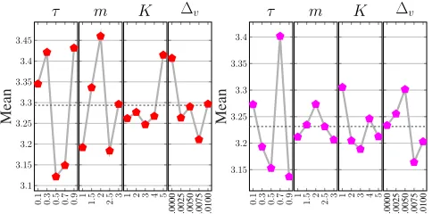
Fig. 1: Main effects plots for HH-LA (left) and HH-RILA (right) for each parameter: exploration phase (τ), multiplier (m), maximum iterations (K) for applying a low leve MOEA, and hypervolume improvement threshold (∆v).

level MOEA, and hypervolume improvement threshold ∆v.

Five different values for each parameter are considered: τ ∈ {0.1, 0.3, 0.5, 0.7, 0.9},m∈ {1.0, 1.5, 2.0, 2.5, 3.0},K{1, 2, 3, 4, 5},∆v∈ {0.0, 0.0025, 0.005, 0.0075, 0.01}. Even with

this sample of five settings for each of the four parameters, 625 parameter tuning experiments would have been required for testing all combinations of the parameter settings. In this study, the Taguchi orthogonal arrays experimental design method ([67], [72]) is used for parameter tuning. Sampling the configurations based on the orthogonal array, denoted as

L25, reduces the number of parameter tuning experiments to

25 configurations for each algorithm, which are tested on the benchmark functions.

The measurement used during the tuning experiments is

µnorm. The original µnorm is defined for the minimisation

problems. Since we are maximising hypervolume, we slightly modify the formulation of µnorm as follows. Let S(x,n)

be the set of hypervolume (30 hypervolume values in our case resulting from 30 trials) obtained by an algorithm x, where x ∈ X on a problem n, where n ∈ N; X and

N are the sets of algorithms and problems, respectively. Let Snmin = M IN∀s∈S(x,n),∀x∈X be the minimum and

Smax

n =M AX∀s∈S(x,n),∀x∈X be the maximum hypervolume

obtained by all the algorithms on a problemn. The normalised hypervolume of an algorithmxon a problemnis computed as

fnorm

(x,n) =

S_nmax−AV Gs∈S_(x,n)(s)

Smax

n −Sminn . The average of

fnorm

(x,n) defined

asµnorm(x) =AV G∀n∈N(f₍norm_x,n))serves as the measurement

for the tuning experiments. The lower theµnorm(x)value, the

better the performance of the algorithmx.

The main effects plots in Figure 1 indicate the mean effect of each parameter setting on the performances of HH-LA and HH-RIHH-LA. The parameter setting that achieves the lowest meanµnormaveraged across all trials using that setting

regardless of the remaining parameter settings would be the best value for that parameter. Thus, the best configuration for HH-LA is{τ = 0.5, m= 2.5, K = 3,∆v = 0.0075}, and for

HH-RILA is{τ = 0.9, m= 3.0, K = 3,∆v = 0.0075}. Both

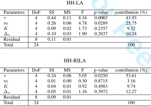
settings are used in this paper for the rest of the experiments. Analysis of Variance (ANOVA) [73] test is performed to observe how sensitive the performance of proposed hyper-heuristics to the parametric settings is by looking into the

For Peer Review

significance and contribution (in percentage) of each param-eter. Table I shows that exploration phase parameter τ has the most significant influence on the performance of both HH-LA and HH-RILA at a significance level of 5% (i.e., p-value < 0.05). The parameter τ has the highest percentage contribution of 43.93% and 53.61% to the performance of HH-LA and HH-RIHH-LA, respectively. The reward/penalty multiplier

m also significantly contribute to the performance of HH-LA with the second largest percentage contribution of 25.75%, while this parameter has almost no contribution (3.16%) to the performance of HH-RILA. The remaining two parameters are not significantly influential on the performance of either proposed hyper-heuristics.

TABLE I: ANOVA test to identify the contribution (%) of each parameter for HH-LA and HH-RILA (DoF: degrees of freedom, SS: sum of squares, MS: mean squares, F: variance ratio).

HH-LA

Parameters DoF SS MS F p-value contribution (%)

τ 4 0.44 0.11 8.16 0.0063 43.93

m 4 0.26 0.06 4.78 0.0289 25.75

K 4 0.09 0.02 1.73 0.2357 9.32

∆v 4 0.10 0.03 1.90 0.2037 10.24

Residual 8 0.11 0.01

Total 24 100

HH-RILA

Parameters DoF SS MS F p-value contribution (%)

τ 4 0.24 0.06 5.05 0.0250 53.61

m 4 0.01 0.00 0.30 0.8715 3.16

K 4 0.04 0.01 0.92 0.4983 9.74

∆v 4 0.05 0.01 1.16 0.3972 12.27

Residual 8 0.09 0.01

Total 24 100

C. Experimental Results on WFG and DTLZ

In this section, we use hypervolume as the main perfor-mance indicator. One-tailed Wilcoxon rank-sum test (also known as Mann-Whitney U test) is applied based on the raw hypervolume values obtained from 30 trials of each algorithm to test if there is a statistically significant performance dif-ference between a pair of algorithms. The significance level is set to 5%. The reference (or nadir) point (denoted as r) for the WFG and DTLZ benchmark problems are chosen as follows. For each WFG problem, the reference point is set as

ri_{= 2i+ 1, wherei= 1,2, ..., kis the index of the objective}

and k is the total objective number. Thus, for each WFG problem, the reference point is (3, 5, 7). The reference point for DTLZ problems is set asri= 0.5for DTLZ1,ri= 1.0for DTLZ2 to DTLZ6 and ri= 1.0 ifi < k, otherwise,rk= 2k

for DTLZ7.

The convergence indicator + is utilised as an additional performance comparison indicator. We notice that in some cases, the performance differences between algorithms are not distinguishable if the raw values are plotted directly. Here only for the visualisation purposes, we map the raw hypervolume/+value into the range of [0,1] via normalisation

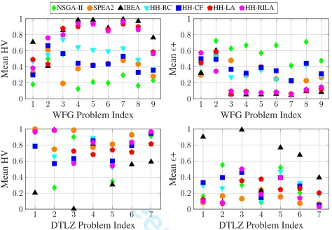
using the extreme (minimum and maximum) values collected from all algorithms over 30 trials on each instance, then the mean hypervolume and + values are plotted in Figure 2. Higher the hypervolume or lower the+value means a better performance.

Figure 2 shows that IBEA performs the best on WFG benchmark with respect to both hypervolume and + in the overall. HH-RILA and HH-LA follow the performance of IBEA closely. NSGA-II clearly performs the worst on WFG. The performance of IBEA gets much poorer and becomes overall the worst approach for the DTLZ benchmark func-tions with respect to both metrics. SPEA2 performs the best on over half of DTLZ benchmark. HH-RILA and HH-LA always achieve the second best performance on most DTLZ benchmark or even the best on DTLZ7. In addition, the hypervolume based performance ranking of all algorithms on each benchmark problem is almost fully consistent with the+

based ranking except for WFG1. On WFG1, IBEA achieves the best rank with respect to hypervolume, however, IBEA performs slightly worse than SPEA2 on WFG1 with respect to the+indicator. This inconsistency, also discussed in [60], is possibly due to the different working principles of both indicators.

One-tailed Wilcoxon rank-sum test at 5% significance level is conducted on the performance of each pair of algorithms with respect to hypervolume. The statistical test results are summarised in Table II and we have the following observa-tions.

In the overall, both of our MOHHs deliver a better perfor-mance than any of the individual MOEAs run on its own on the WFG and DTLZ benchmarks. The statistical test results show that HH-LA and HH-RILA outperform NSGA-II on all nine WFG benchmark functions while 3 out of 7DTLZ problems, including DTLZ1-2 and DTLZ5. HH-RILA addi-tionally performs significantly better than NSGA-II on DTLZ6 and DTLZ7. HH-LA and HH-RILA perform significantly better than SPEA2 on the same 8 out of 9 WFG benchmark functions including WFG1, WFG3-9. HH-RILA additionally outperforms SPEA2 on DTLZ2 and DTLZ7. Although IBEA delivers a good overall performance on the WFG benchmark, both our algorithms still manage to outperform IBEA on 5 out of 7 DTLZ problems including DTLZ1, DTLZ3 and DTLZ5-7. HH-RILA also performs significantly better than IBEA on WFG2.

Both LA and RILA outperform CF and HH-RC. Specifically, both of our hyper-heuristics perform sig-nificantly better than HH-CF on 11 benchmark functions out of total 16, including the same eight WFG benchmark functions (WFG1, WFG3-9) and three DTLZ benchmark functions (DTLZ1-3 for HH-LA, while DTLZ1-2 and DTLZ6 for HH-RILA). The performance difference between each of the proposed hyper-heuristics and HH-RC is statistically sig-nificant with respect to hypervolume on 10 out of 16 problems which include the same seven WFG benchmark functions (WFG3-9) and three slightly different DTLZ problems: HH-LA outperforms HH-RC on DTLZ1-2 and DTLZ5, while DTLZ1-2 and DTLZ7 for HH-RILA. HH-CF only outperforms HH-RC on DTLZ7, while they perform similarly on 8 out of

For Peer Review

NSGA-II SPEA2 IBEA HH-RC HH-CF HH-LA HH-RILA

1

2

3

4

5

6

7

8

9

0

0

.

2

0

.

4

0

.

6

0

.

8

1

WFG Problem Index

Mean

HV

1

2

3

4

5

6

7

8

9

0

0

.

2

0

.

4

0

.

6

0

.

8

1

WFG Problem Index

Mean

+

1

2

3

4

5

6

7

0

0

.

2

0

.

4

0

.

6

0

.

8

1

DTLZ Problem Index

Mean

HV

1

2

3

4

5

6

7

0

0

.

2

0

.

4

0

.

6

0

.

8

1

DTLZ Problem Index

Mean

+

Fig. 2: Performance comparison of all the algorithms with respect to hypervolume and +on 3D WFG and DTLZ problems. TABLE II: One-tailed Wilcoxon rank-sum test at 5% significance level on WFG and DTLZ benchmark problems with respect to hypervolume. ‘W’ and ‘D’ are short for ‘WFG’ and ‘DTLZ’ respectively. ‘>’ means the significantly better than, ‘<’ significantly worse than, ‘∼’ no significant difference.

W1 W2 W3 W4 W5 W6 W7 W8 W9 D1 D2 D3 D4 D5 D6 D7

HH-LA vs HH-CF > ∼ > > > > > > > > > > ∼ ∼ ∼ ∼

HH-LA vs HH-RC ∼ ∼ > > > > > > > > > ∼ ∼ > ∼ ∼

HH-LA vs NSGA-II > > > > > > > > > > > ∼ ∼ > ∼ < HH-LA vs SPEA2 > ∼ > > > > > > > < < < ∼ < < < HH-LA vs IBEA < ∼ ∼ < < ∼ < < < > ∼ > ∼ > > >

HH-CF vs HH-RC < ∼ < < < < < < ∼ ∼ ∼ ∼ ∼ ∼ ∼ >

HH-RILA vs HH-CF > ∼ > > > > > > > > > ∼ ∼ ∼ > ∼

HH-RILA vs HH-RC ∼ ∼ > > > > > > > > > ∼ ∼ ∼ ∼ > HH-RILA vs HH-LA < > < > ∼ < > < ∼ > ∼ ∼ ∼ < > ∼

HH-RILA vs NSGA-II > > > > > > > > > > > < ∼ > > > HH-RILA vs SPEA2 > ∼ > > > > > > > < > < ∼ < < > HH-RILA vs IBEA < > < < < < < < < > ∼ > ∼ > > > NSGA-II vs SPEA2 < ∼ > < < < < < ∼ < < < > < < < NSGA-II vs IBEA < ∼ < < < < < < < > < > > ∼ > > SPEA2 vs IBEA < ∼ < < < < < < < > < > < > > >

16 problems (WFG2, WFG9 and DTLZ1-6). HH-CF delivers a significantly worse performance than HH-RC on the rest of the seven problems (WFG1 and WFG3-8).

As for the performance comparison between HH-LA and HH-RILA, HH-LA is slightly better than HH-RILA in the overall on the WFG problems. This performance difference is statistically significant on four WFG problems including WFG1, WFG3, WFG6 and WFG8, while HH-RILA performs significantly better than HH-LA on three WFG problems: WFG2, WFG4 and WFG7. However, considering DTLZ

benchmark, HH-RILA performs slightly better than HH-LA in the overall. This performance difference is statistically signif-icant on DTLZ1 and DTLZ6, while HH-LA only outperforms HH-RILA on DTLZ5.

D. Analysis of Hyper-heuristics on WFG and DTLZ

1) Utilisation of Low Level Metaheuristics: The ‘utilisation rate’ of a low level metaheuristic is the number of invocations of this metaheuristic divided by the total number of meta-heuristic selection decision points in a given trial. The mean

For Peer Review

NSGA-II SPEA2 IBEA

HH-CF

0 0.2 0.4 0.6 0.8 1 W1 W2 W3 W4 W5 W6 W7 W8 W9 HH-RILA

0 0.2 0.4 0.6 0.8 1 W1 W2 W3 W4 W5 W6 W7 W8 W9 HH-LA

0 0.2 0.4 0.6 0.8 1 W1 W2 W3 W4 W5 W6 W7 W8 W9 HH-CF

0 0.2 0.4 0.6 0.8 1 D1 D2 D3 D4 D5 D6 D7 HH-RILA

0 0.2 0.4 0.6 0.8 1 D1 D2 D3 D4 D5 D6 D7 HH-LA

0 0.2 0.4 0.6 0.8 1 D1 D2 D3 D4 D5 D6 D7

Fig. 3: The mean utilisation rate of each metaheuristic by HH-LA (left), HH-RIHH-LA (middle) and HH-CF (right) over 30 trials on WFG (‘W’) and DTLZ (‘D’).

utilisation rates of the three MOEAs i.e., NSGA-II, SPEA2 and IBEA averaged over 30 trials on the WFG and DTLZ benchmark functions produced by LA, RILA and HH-CF [14] are illustrated in Figure 3.

Figure 3 shows the differences in learning characteristics of these three online learning MOHHs. Firstly, HH-LA and HH-RILA provide a bias towards using the best performing MOEA with respect to hypervolume. Specifically, both HH-LA and HH-RIHH-LA choose IBEA and SPEA2 more frequently while solving the WFG and DTLZ problems, respectively. This is not surprising, considering that hypervolume serves as the main guidance in the learning mechanisms of our hyper-heuristics. Secondly, in certain cases, such as WFG4-8 and DTLZ6, HH-RILA almost exclude NSGA-II which is the worst performed MOEA on those problems. Interestingly, HH-CF generates a similar utilisation rate for low level MOEAs across different problem sets. On average, HH-CF uses NSGA-II, SPEA2 and IBEA for 40%, 40% and 20% of all the decision points, respectively, on the WFG benchmark. Similarly, HH-CF uses NSGA-II, SPEA2 and IBEA for 34%, 38% and 28%, respectively, on the DTLZ benchmark. This might indicate that the adaptation mechanism in HH-CF has some issues controlling these three low level metaheuristics properly on different problem instances.

2) An Analysis of the Transition Probabilities: The pro-posed hyper-heuristics embed a learning mechanism which maintains the transition probabilities between any pair of MOEAs. Figure 4 provides the final transition probability matrices obtained by HH-LA and HH-RILA averaged over 30 trials for the sample cases of WFG7 and DTLZ3.

Figure 4 illustrates that both HH-LA and HH-RILA yield higher probability entries preferring transitions to IBEA than to other MOEAs for WFG7. This is consistent with the performance assessment of each individual MOEA (Figure 2), which shows that IBEA performs the best on WFG7. Moreover, HH-RILA excludes the worst performing MOEA i.e., NSGA-II after the initialisation stage for solving WFG7. This is likely the reason why HH-RILA performs significantly better than HH-LA on WFG7.

DTLZ3 is an interesting case. IBEA delivers a better

perfor-NSGA-II SPEA2 IBEA

IBEA SPEA2 NSGA-II HH-LA DTLZ3 0.42 0.38 0.40 0.35 0.31 0.37 0.24 0.31 0.23

NSGA-II SPEA2 IBEA

IBEA SPEA2 NSGA-II HH-LA WFG7 0.19 0.22 0.25 0.19 0.29 0.37 0.62 0.49 0.39

NSGA-II SPEA2 IBEA

IBEA SPEA2 NSGA-II HH-RILA DTLZ3 0.38 0.17 0.65 0.16 0.44 0.09 0.46 0.39 0.26 0 0.1 0.2 0.3 0.4 0.5 0.6 0.7 NSGA-II SPEA2 IBEA

IBEA SPEA2 NSGA-II HH-RILA WFG7 0.00 0.00 0.00 0.22 0.21 0.00 0.78 0.79 0.00

Fig. 4: The averaged transition probability matrices (over 30 trials) produced by HH-LA (left column) and HH-RILA (right column) while solving WFG7 and DTLZ3. The lighter the colour, the higher the transition probability.

mance in the early stages, but stagnates and even deteriorates later during the search process. Due to the misleading perfor-mance of IBEA in the early stage, HH-RILA rewards IBEA more than the other MOEAs, while excluding the ones with potentially good performance, such as, SPEA2. Consequently, RILA ends up performing significantly worse than HH-LA on DTLZ3.

In summary, the proposed learning mechanism is capable of adaptively updating the transition probabilities between pairs of MOEAs giving bias towards the right algorithms (with good performance) during the search process in an online manner. Moreover, the ranking initialisation scheme is, in some cases, capable of improving the overall performance significantly by detecting and excluding potentially poor performing MOEA(s) in the early stages of the search.

3) An Analysis of Approximate Pareto Fronts: So far, IBEA is a strong competitor of HH-LA and HH-RILA with respect to hypervolume. To get more insights on the distribution of solutions from IBEA and the proposed hyper-heuristics, PFs obtained from HH-RILA and IBEA for WFG7 and DTLZ3 are illustrated in Figure 5. HH-LA produces PFs very similar to RILA on almost all problems, and so we focus on HH-RILA here.

Figure 5 demonstrates that IBEA is prone to be trapped at a local optimum. IBEA produces uneven solution distribution for WFG7, leaving clear gaps between the boundary and inner regions, whereas HH-RILA reaches a better solution distribution for this problem.

IBEA performs poorly on DTLZ3. All the solutions are clustered around the ‘corner’ points which suggests that the performance of IBEA degrades during the search process. This interesting behaviour of IBEA has also been observed previously by Tuˇsaret al. [69] (in Figure 7) and [74]. More importantly, solutions from HH-RILA clearly spread much more evenly on the front than IBEA, possibly due to the utilisation of multiple MOEAs.

For Peer Review

0 0

2 1

HH-RILA

4 2 5

0

0 0

1 2

IBEA

2 4 5

(a) WFG7

0

0 0

0.5 0.5

0.5

HH-RILA

1 1 1

0

0 0

0.5 0.5

0.5

IBEA

1 1 1

(b) DTLZ3

Fig. 5: Approximate PFs produced by HH-RILA (left column) and IBEA (right column) on WFG7 and DTLZ3.

NSGA-II SPEA2 IBEA

0 10 20 30 40 50 0

5 10 15 20 25 30

Iterations

Number

of

In

v

ocations

HH-LA WFG7

0 10 20 30 40 50 0

5 10 15 20 25 30

Iterations

Number

of

In

v

ocations

HH-RILA WFG7

0 10 20 30 40 50 60 70 80 90 100 0

5 10 15 20 25 30

Iterations

Number

of

In

v

ocations

HH-LA DTLZ3

0 10 20 30 40 50 60 70 80 90 100 0

5 10 15 20 25 30

Iterations

Number

of

In

v

ocations

HH-RILA DTLZ3

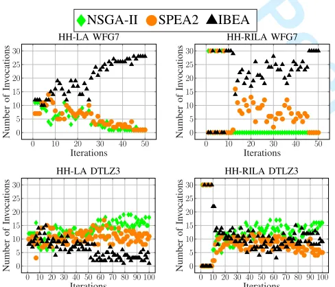
Fig. 6: The number of invocations of each MOEA at each iteration over 30 trials on WFG7 and DTLZ3 obtained from HH-LA (left column) and HH-RILA (right column).

4) An Analysis of Search Dynamics: To have a further understanding of the search progress induced by each low level MOEA at each trial under the proposed hyper-heuristics, we recorded which MOEA was chosen and applied at each iteration of 30 trials. Figure 6 provides plots based on that data as a representative of the search dynamics for HH-LA and HH-RILA on WFG7 and DTLZ3. Each tick on the plot indicates the total number of trials that the relevant MOEA is selected and invoked by the indicated hyper-heuristic at a given iteration. For example, HH-LA calls NSGA-II, 11 times, SPEA2, 7 times and IBEA, 12 times at the first iteration out of 30 trials when solving WFG7.

As observed from Figure 6, HH-LA slowly reduces the

usage of poor performing MOEAs which are NSGA-II and SPEA2 for WFG7 during the exploration phase which corre-sponds to the first half of the search process (τ=0.5). Then the best performing MOEA; i.e., IBEA is predominately used for the remaining iterations. Meanwhile, HH-RILA excludes NSGA-II after the initial ranking stage (first nine iterations). Following the exploration phase, HH-RILA prefers invoking IBEA more and more while SPEA2 less and less as the search progresses. This behaviour is also reflected on the transition probability matrix (Figure 4). The transition probabilities from any MOEA to IBEA are higher than to the other MOEAs for both HH-LA and HH-RILA. Moreover, the transition probabilities to and from NSGA-II are all 0s for HH-RILA on WFG7.

On DTLZ3, HH-LA tends to prefer employing, firstly, NSGA-II and then SPEA2 more than IBEA after the ex-ploration phase. Nevertheless, HH-RILA cannot detect the degrading performance of IBEA rapidly enough during the search, and this results in excluding SPEA2 or NSGA-II in some trials. Therefore, the performance of HH-RILA becomes worse than HH-LA with respect to hypervolume. This be-haviour is also consistent with the mean utilisation rates as provided in Figure 3, which shows that HH-LA uses NSGA-II and SPAE2 more than HH-RILA does on DTLZ3.

E. Experimental Results for Vehicle Crashworthiness

HH-LA and HH-RILA are also tested on the real-world problem of VCP. The same experimental settings as in [14] are used for a fair performance comparison. The population size is fixed as 30 in these experiments. Each iteration consists of 50 generations. Each algorithm terminates whenever 75,000 solution evaluations are exceeded. The reference point for each VC instance is set to ri _{= z}nadiri _{+ 0.5(z}nadiri _−zideali_),

where i is the index of an objective, znadiri _{and z}ideali

are the nadir (highest) and ideal (lowest) value of objective

i, respectively. The performances of each algorithm with respect to hypervolume and + are provided in Table III. The results show that NSGA-II performs the best (with the highest hypervolume and lowest+) on VC1 and VC2, while HH-RILA performs the best on VC3 and VC4 based on both performance indicators when compared to the other algorithms including each MOEA used on its own. The proposed hyper-heuristic exploits the synergy between MOEAs with different performances leading to an improved overall performance.

The one-tailed Wilcoxon rank-sum test comparing the per-formance difference of all pairs of multiobjective approaches are summarised in Table IV). The results suggest that both NSGA-II and SPEA2 perform significantly better than IBEA. HH-RILA outperforms HH-CF on 2 out of 4 VC problem instances (VC3 and VC4), and HH-RC on 3 out of 4 VC problem instances (VC2-4), and beats IBEA on all four VC problems. HH-LA performs similar as HH-CF, significantly better HH-RC on VC2, and also outperforms IBEA on all four VC problems. HH-RILA outperforms HH-LA on VC2-4.

F. Generality Analysis

Different approaches perform the best on different problems. The cross-domain search performance of algorithms indicating

For Peer Review

TABLE III: MeanST D hypervolume and+values for the vehicle crashworthiness problems, averaged over 30 trials and their

standard deviations provided as subscript entries. The best mean hypervolume and +on each problem instance is highlight in bold.

Hypervolume +

VC1 VC2 VC3 VC4 VC1 VC2 VC3 VC4

HH-LA 98.06931.55 53.07152.35 1.65530.10 2.05580.07 0.13540.04 0.07170.12 0.35650.13 0.08440.07

HH-RILA 98.82091.94 53.77291.26 1.77780.11 2.09240.03 0.12250.05 0.03740.06 0.19950.15 0.04950.03

HH-CF 98.90381.82 53.56281.74 1.66960.11 2.05820.05 0.11940.05 0.05010.09 0.33720.14 0.07940.05

HH-RC 98.25661.75 52.64602.78 1.71820.13 2.04570.06 0.13800.04 0.09820.14 0.27380.16 0.08970.06

NSGA-II 100.21631.48 53.95140.04 1.70930.12 2.08800.04 0.10070.04 0.03620.00 0.28640.16 0.05520.04

SPEA2 99.5532.02 53.65231.76 1.72780.12 2.06690.05 0.11880.05 0.04860.09 0.26510.16 0.08180.06

IBEA 96.94350.57 52.14653.06 1.68460.13 2.02130.06 0.1570.02 0.11840.16 0.31190.16 0.11480.06

TABLE IV: One-tailed Wilcoxon rank-sum test at 5% signifi-cance level on VC problems with respect to hypervolume.‘>’ means the significantly better than, ‘<’ significantly worse than, ‘∼’ no significant difference.

VC1 VC2 VC3 VC4

HH-LA vs HH-CF ∼ ∼ ∼ ∼

HH-LA vs HH-RC ∼ > ∼ ∼

HH-LA vs NSGA-II < < ∼ <

HH-LA vs SPEA2 ∼ ∼ ∼ ∼

HH-LA vs IBEA > > ∼ > HH-RILA vs HH-CF ∼ ∼ > > HH-RILA vs HH-RC ∼ > > > HH-RILA vs HH-LA ∼ > > > HH-RILA vs NSGA-II < < > ∼

HH-RILA vs SPEA2 ∼ > ∼ > HH-RILA vs IBEA > > > >

HH-CF vs HH-RC ∼ ∼ < ∼

NSGA-II vs SPEA2 ∼ > < > NSGA-II vs IBEA > > > > SPEA2 vs IBEA > > > >

which algorithm is more general and the best across a range of problems is often of interest [7]. As mentioned before,

µnorm is used in this work to assess the generality level of an

algorithm across different problems including the benchmark functions and vehicle crashworthiness problems.

The empirical results based on µnorm are presented in

Table V. We also rank all the algorithms with respect to

µnorm values. The lower µnorm value is, the better the

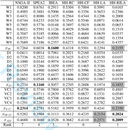
rank of an algorithm. From Table V, we have the following observations. There is no single MOEA performing well across all three problem domains even though each uses the same perturbative operators. The performance of each individual MOEA varies vastly on different domains. IBEA, SPEA2 and NSGA-II deliver the best performance on WFG, DTLZ and VC, respectively. Although HH-RILA is always the second best performing approach on each domain, it has the best cross-domain performance and so the most general approach among all algorithms tested in this study with a mean

µnorm of 0.2089 based on the results from all 20 problem

instances. Moreover, HH-LA turns out to be the second best approach with a mean µnorm of 0.2571. The cross-domain

performance of our selection hyper-heuristics are followed by IBEA, SPEA2, HH-RC, HH-CF and NSGA-II in that order. If we consider only WFG and DTLZ benchmarks ignoring the vehicle crashworthiness problem and compare the cross-domain performance of all algorithms, HH-RILA and HH-LA still rank the best and the second best based on the mean

TABLE V: Hypervolume µnorm for each algorithm on each

test problem instance. x¯W,x¯D,x¯V C,x¯W D, andx¯All denote

the meanµnormon WFG, DTLZ, VC, both WFG and DTLZ,

as well as all three problem domains, respectively. The best mean µnorm on each benchmark is highlight in bold, the

second best is in gray box.

NSGA-II SPEA2 IBEA HH-RC HH-CF HH-LA HH-RILA W1 0.8200 0.6761 0.2911 0.5304 0.7004 0.5091 0.6165 W2 0.4985 0.3881 0.5906 0.4486 0.3356 0.5653 0.2386 W3 0.4431 0.8086 0.1435 0.2564 0.4344 0.1206 0.2008 W4 0.8744 0.6233 0.0154 0.3545 0.5546 0.0971 0.0614 W5 0.7905 0.5776 0.0148 0.3897 0.5819 0.0630 0.0653 W6 0.8021 0.5591 0.1126 0.4029 0.5648 0.1318 0.1519 W7 0.7047 0.5185 0.0066 0.3662 0.4684 0.0639 0.0337 W8 0.8353 0.5647 0.0295 0.5101 0.6688 0.1002 0.1354 W9 0.7689 0.7186 0.2357 0.6273 0.6421 0.4141 0.4357

¯

xW 0.7264 0.6038 0.1600 0.4318 0.5501 0.2294 0.2155

D1 0.0411 0.0014 0.7981 0.2021 0.2160 0.0354 0.0335 D2 0.7336 0.2522 0.0114 0.3425 0.4315 0.0150 0.0107 D3 0.1000 0.0144 0.9974 0.4164 0.3687 0.2753 0.4280 D4 0.1327 0.2266 0.1859 0.1092 0.1465 0.3186 0.1669 D5 0.6549 0.1900 0.6945 0.4757 0.3996 0.2622 0.4605 D6 0.1654 0.0729 0.4437 0.1606 0.2082 0.2882 0.1654 D7 0.0862 0.0548 0.4093 0.1866 0.0550 0.1867 0.0339

¯

xD 0.2734 0.1160 0.5057 0.2705 0.2608 0.1974 0.1855

VC1 0.2715 0.3746 0.7804 0.5762 0.4756 0.6054 0.4885 VC2 0.0288 0.0711 0.2839 0.2133 0.0837 0.1531 0.0540 VC3 0.4961 0.4402 0.5708 0.4693 0.6164 0.6596 0.2887 VC4 0.1291 0.2265 0.4378 0.3247 0.2672 0.2782 0.1088

¯

xV C 0.2314 0.2781 0.5182 0.3959 0.3607 0.4241 0.2350

¯

xW D 0.5282 0.3904 0.3113 0.3612 0.4235 0.2154 0.2024

¯

xAll 0.4688 0.3680 0.3526 0.3682 0.4110 0.2571 0.2089

Rank 7 4 3 5 6 2 1

µnormvalues averaged over all benchmark functions, yielding

0.2024 and 0.2154, respectively.

V. CONCLUSION ANDFUTUREWORK

In this study, we proposed two variants of a learning au-tomata based multiobjective selection hyper-heuristic: HH-LA and HH-RILA. The performance and generality of HH-LA and HH-RILA controlling three MOEAs are investigated on three multiobjective continuous optimisation problem domains, in-cluding two sets of benchmark functions (WFG and DTLZ) and the real-world problem of vehicle crashworthiness. The experimental results show that the different MOEAs perform the best on different problem domains. However, HH-RILA and HH-LA perform the best and second best, respectively, across all test problem instances based on theµnormindicator.