Value based Search in Execution Space for Mapping Instructions to Programs

1942

Value-based Search in Execution Space for Mapping Instructions to

Programs

Dor Muhlgay1 Jonathan Herzig1 Jonathan Berant1,2

1_{School of Computer Science, Tel-Aviv University}

2_{Allen Institute for Artificial Intelligence}

{dormuhlg@mail,jonathan.herzig@cs,joberant@cs}.tau.ac.il

Abstract

Training models to map natural language in-structions to programs, given target world su-pervision only, requires searching for good programs at training time. Search is com-monly done using beam search in the space of partial programs or program trees, but as the length of the instructions grows finding a good program becomes difficult. In this work, we propose a search algorithm that uses the target world state, known at training time, to train acriticnetwork that predicts the expected reward of every search state. We then score search states on the beam by interpolating their expected reward with the likelihood of pro-grams represented by the search state. More-over, we search not in the space of programs but in a more compressed state of program ex-ecutions, augmented with recent entities and actions. On the SCONE dataset, we show that our algorithm dramatically improves perfor-mance on all three domains compared to stan-dard beam search and other baselines.

1 Introduction

Training models that can understand natural lan-guage instructions and execute them in a real-world environment is of paramount importance for communicating with virtual assistants and robots, and therefore has attracted considerable atten-tion (Branavan et al., 2009; Vogel and Jurafsky, 2010; Chen and Mooney, 2011). A prominent ap-proach is to cast the problem as semantic parsing, where instructions are mapped to a high-level pro-gramming language (Artzi and Zettlemoyer, 2013; Long et al., 2016; Guu et al., 2017). Because anno-tating programs at scale is impractical, it is desir-able to train a model from instructions, an initial world state, and a target world state only, letting the program itself be a latent variable.

Learning from such weak supervision results in a difficult search problem at training time. The

model must search for a program that when ex-ecuted leads to the correct target state. Early work employed lexicons and grammars to con-strain the search space (Clarke et al., 2010; Liang et al., 2011; Krishnamurthy and Mitchell, 2012; Berant et al., 2013; Artzi and Zettlemoyer, 2013), but recent success of sequence-to-sequence mod-els (Sutskever et al., 2014) shifted most of the bur-den to learning. Search is often performed sim-ply using beam search, where program tokens are emitted from left-to-right, or program trees are generated top-down (Krishnamurthy et al., 2017; Yin and Neubig, 2017; Cheng et al., 2017; Ra-binovich et al., 2017) or bottom-up (Liang et al., 2017; Guu et al., 2017; Goldman et al., 2018). Nevertheless, when instructions are long and com-plex and reward is sparse, the model may never find enough correct programs, and training will fail.

In this paper, we propose a novel search algo-rithm for mapping a sequence of natural language instructions to a program, which extends the stan-dard beam-search in two ways. First, we capitalize on the target world state being available at training time and train acriticnetwork that given the lan-guage instructions, current world state, and target world state estimates the expected future reward for each search state. In contrast to traditional beam search where states representing partial pro-grams are scored based on their likelihood only, we also consider expected future reward, leading to a more targeted search at training time. Sec-ond, rather than search in the space of programs, we search in a more compressed execution space, where each state is defined by a partial program’s execution result.

search gets stuck in local optima and is unable to discover good programs for many examples, our model is able to bootstrap, improving final perfor-mance by 20 points on average. We also perform extensive analysis and show that both value-based search as well as searching in execution space con-tribute to the final performance. Our code and

data are available at http://gitlab.com/

tau-nlp/vbsix-lang2program.

2 Background

Mapping instructions to programs invariably in-volves acontext, such as a database or a robotic en-vironment, in which the program (or logical form) is executed. The goal is to train a model given a training set{(x(j)= (c(j),u(j)), y(j))}Nj=1, where

c is the context, u is a sequence of natural lan-guage instructions, and y is the target state of the environment after following the instructions, which we refer to as denotation. The model is trained to map the instructions u to a programz

such that executing z in the context c results in the denotationy, which we denote by_Jz_Kc = y. Thus, the program z is a latent variable we must search for at both training and test time. When the sequence of instructions is long, search becomes hard, particularly in the early stages of training.

Recent work tackled the training problem us-ing variants of reinforcement learnus-ing (RL) (Suhr and Artzi, 2018; Liang et al., 2018) or maximum marginal likelihood (MML) (Guu et al., 2017; Goldman et al., 2018). We now briefly describe MML training, which we base our training proce-dure on, and outperformed RL in past work under comparable conditions (Guu et al., 2017).

We denote by πθ(·)a model, parameterized by

θ, that generates the program z token by token from left to right. The modelπθ receives the

con-textc, instructionsu and previously predicted to-kens z1...t−1, and returns a distribution over the

next program tokenzt. The probability of a

pro-gram prefix is defined to be: pθ(z1...t | u, c) =

Qt

i=1πθ(zi | u, c, z1...i−1). The model is trained

to maximize the MML objective:

JM M L= log

Y

(c,u,y)

pθ(y|c,u) =

X

(c,u,y)

log(X

z

pθ(z|u, c)·R(z)),

whereR(z) = 1ifJzKc=y, and 0 otherwise (For

brevity, we omit c and y fromR(·)). Typically,

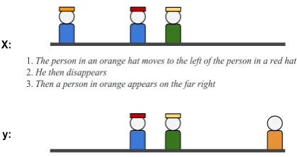
1. The person in an orange hat moves to the left of the person in a red hat

2. He then disappears

3. Then a person in orange appears on the far right

X:

y:

Figure 1: Example from the SCENEdomain in SCONE (3 utterances), where people with different hats and shirts are located in different positions. The example contains (from top to bottom): an initial world (the peo-ple’s properties, from left to right: a blue shirt with an orange hat, a blue shirt with a red hat, and a green shirt with a yellow hat), a sequence of natural language in-structions, and a target world (the people’s properties, from left to right: blue shirt with a red hat, green shirt with a yellow hat, and an orange shirt).

the MML objective is optimized with stochastic gradient ascent, where the gradient for an example (c,u, y)is:

∇θJM M L=

X

z

q(z)·R(z)∇θlogpθ(z|c,u)

q(z) := PR(z)·pθ(z|c,u)

˜

zR(˜z)·pθ(˜z|c,u)

.

The search problem arises because it is impos-sible to enumerate the set of all programs, and thus the sum over programs is approximated by a small set of high probability programs, which have high weightsq(·)that dominate the gradient. Search is commonly done with beam-search, an iterative algorithm that builds an approximation of the highest probability programs according to the model. At each time step t, the algorithm con-structs a beamBtof at mostK program prefixes

of lengtht. Given a beamBt−1,Btis constructed

by selecting the K most likely continuations of prefixes inBt−1 , according topθ(z1..t|·). The

al-gorithm runsLiterations, and returns all complete programs discovered.

1 2 3

Program stack (𝜓): Command history (h):

World state (w0

): Current utterance (u1

):

The person in the yellow hat moves to the left of the person in blue

1 2 3

Program stack (𝜓): Command history (h):

World state (w1

): Current utterance (u2

): Then he disappears

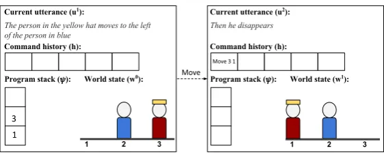
Figure 2: An illustration of a state transition in SCONE.πθpredicted the action tokenMOVE. Before the transition (left), the command history is empty and the program stack contains the arguments 3 and 1, which were computed in previous steps. Note that the state does not include the partial program that computed those arguments. After transition (right), the executor popped the arguments from the program stack and applied the actionMOVE3 1: the man in position 3 (a person with a yellow hat and a red shirt) moved to position 1 (to the left of the person with the blue shirt), and the action is added to the execution history with its arguments. Since this action terminated the command,πθadvanced to the next utterance.

The SCONE dataset Long et al. (2016) pre-sented the SCONE dataset, where a sequence of instructions needs to be mapped to a program con-sisting of a sequence of executable commands. The dataset has three domains, where each do-main includes several objects (such as people or beakers), each with different properties (such as shirt color orchemical color). SCONE provides a good environment for stress-testing search al-gorithms because a long sequence of instructions needs to be mapped to a program. Figure 1 shows an example from the SCENEdomain.

Formally, the context in SCONE is a world specified by a list of positions, where each po-sition may contain an object with certain prop-erties. A formal language is defined to inter-act with the world. The formal language con-tains constants (e.g., numbers and colors), func-tions that allow to query the world and re-fer to objects and intermediate computations, and actions, which are functions that modify the world state. Each command is composed of a single action and several arguments con-structed recursively from constants and functions. E.g., the command MOVE(HASHAT(YELLOW), LEFTOF(HASSHIRT(BLUE))), contains the ac-tion MOVE, which moves a person to a

spec-ified position. The person is computed by

HASHAT(YELLOW), which queries the world

for the position of the person with a yellow hat, and the target position is computed by LEFTOF(HASSHIRT(BLUE)). We refer to Guu et al. (2017) for a full description of the language. Our goal is to train a model that given an ini-tial worldw0 and a sequence of natural language

utterancesu = (u1_{, . . . , u}M_{), will map each}

ut-teranceuito a commandzi such that applying the programz= (z1, . . . , zM)onw0will result in the target world, i.e.,JzKw0 =wM =y.

3 Markov Decision Process Formulation

To present our algorithm, we first formulate the problem as a Markov Decision Process (MDP), which is a tuple(S,A, R, δ). To define the state set S, we assume all program prefixes are exe-cutable, which can be easily done as we show be-low. Theexecution resultof a prefixz˜in the con-text c, denoted by Jz˜K

ex

c , contains its denotation

and additional information stored in the executor. LetZ_prebe the set of all valid programs prefixes. The set of states is defined to beS ={(x,_Jz˜_Kex_c )| ˜

z ∈ Zpre}, i.e., the input paired with all possible execution results.

The action set Aincludes all possible program tokens1, and the transition functionδ :S×A → S is computed by the executor. Last, the reward

R(s, a) = 1 iff the action a ends the program

and leads to a stateδ(s, a)where the denotation is equal to the targety. The modelπθ(·)is a

parame-terized policy that provides a distribution over the program vocabulary at each time step.

SCONE as an MDP We define the partial ex-ecution result Jz˜K

ex

c in SCONE, as described by

Guu et al. (2017). We assume that SCONE’s

formal language is written in postfix notations, e.g., the instruction MOVE(HASHAT(YELLOW), LEFTOF(HASSHIRT(BLUE))) is written as YEL

-LOW HASHAT BLUE HASSHIRT LEFTOF MOVE.

With this notation, a partial program can be exe-cuted left-to-right by maintaining aprogram stack,

ψ. The executor pushes constants (YELLOW) toψ, and applies functions (HASHAT) by popping their arguments fromψand pushing back the computed result. Actions (MOVE) are applied by popping ar-guments fromψand performing the action in the current world.

To handle references to previously executed commands, SCONE’s formal language includes functions that provide access to actions and argu-ments in previous commands. To this end, the executor maintains an execution history, hi = (e1_{, . . . , e}i_{), a list of executed actions and their}

ar-guments. Thus, the execution result of a program prefix is_Jz˜_Kex_w0 = (wi−1, ψ,hi−1).

We adopt the model from Guu et al. (2017) (ar-chitecture details in appendix A): The policy πθ

observes ψ and ui, the current utterance being parsed, and predicts a token. When the model predicts an action token that terminates a com-mand, the model moves to the next utterance (un-til all utterances have been processed). The model uses functions to query the worldwi−1and history

hi−1. Thus, each MDP state in SCONE is a pair

s= (ui,_Jz˜_Kex_w0). Figure 2 illustrates a state transi-tion in the SCENEdomain. Importantly, the state does not store the full program’s prefix, and many different prefixes may lead to the same state. Next, we describe a search algorithm for this MDP.

4 Searching in Execution Space

Model improvement relies on generating correct programs given a possibly weak model. Stan-dard beam-search explores the space of all pro-gram token sequences up to some fixed length. We propose two technical contributions to improve search: (a) We simplify the search problem by searching for correct executions rather than correct programs; (b) We use the target denotation at train-ing time to better estimate partial program scores in the search space. We describe those next.

4.1 Reducing program search to execution search

Program space can be formalized as a directed tree

T = (VT,ET), where vertices VT are program

prefixes, and labeled edgesE_T represent prefixes’ continuations: an edge e = (˜z,z˜0) labeled with the tokena, represents a continuation of the prefix ˜

zwith the tokena, which yields the prefixz˜0. The

red yellow

hasHat

hasShirt

blue

hasShirt

leftOf

move blue

hasShirt

leftOf

move 1

move

Program search space Execution search space red

hasHat hasShirt

1 blue

hasShirt

leftOf

move yellow

1

move

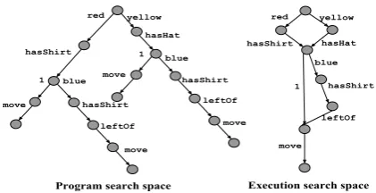
Figure 3: A set of commands represented in program space (left) and execution space (right). The commands relate to the first world in Figure 2. Since multiple prefixes have the same execution result (e.g.,YELLOW HASHATandRED HASSHIRT), the execution space is smaller.

root of the graph represents the empty sequence. Similarly,Execution spaceis a directed graphG= (VG,EG)induced from the MDP described in

Sec-tion 3. VerticesV_G represent MDP states, which express execution results, and labeled edges E_G represent transitions. An edge(s1, s2)labeled by

token a means that δ(s1, a) = s2. Since

multi-ple programs have the same execution result, ex-ecution space is a compressed representation of program space. Figure 3 shows a few commands in both program and execution space. Execution space is smaller, and so searching in it is easier.

Each path in execution space represents a differ-ent program prefix, and the path’s final state rep-resents its execution result. Program search can therefore be reduced to execution search: given an example(c,u, y) and a modelπθ, we can use πθ

to explore in execution space, discovercorrect ter-minal states, i.e. states corresponding to correct full programs, and extract paths leading to those states. As the number of paths may be exponential in the size of the graph, we can use beam-search to extract the most probable correct programs (ac-cording to the model) in the discovered graph.

Our approach is similar to the DPD algo-rithm (Pasupat and Liang, 2016), where CKY-style search is performed in denotation space, fol-lowed by search in a pruned space of programs. However, DPD was used without learning, and the search was not guided by a trained model, which is a major part of our algorithm.

4.2 Value-based Beam Search in Execution Space

Algorithm 1Program Search with VBSIX

1: functionPROGRAMSEARCH(c,u, y, πθ, Vφ) 2: G,T ←VBSIX(c,u, y, πθ, Vφ)

3: Z ←Find paths inGthat lead to states inTwith beam search

4: ReturnZ

5: functionVBSIX(c,u, y, πθ, Vφ)

6: T ← ∅, P← {} .init terminal states and DP chart

7: s0:=The empty program parsing state

8: B0← {s0}, G= ({s0},∅) .Init beam and graph 9: P0[s0]←1 .The probability ofs0is 1 10: fort∈[1. . . L]do

11: Bt← ∅

12: fors∈Bt−1, a∈ Ado

13: s0←δ(s, a)

14: Add edge(s, s0)toGlabeled witha

15: ifs0is correct terminalthen

16: T ← T ∪ {s0}

17: else

18: Pt[s0]←Pt[s0] +Pt−1[s]·πθ(a|s)

19: Bt←Bt∪ {s0}

20: SortBtby AC-SCORER(·)

21: Bt←Keep the top-Kstates inBt 22: ReturnG,T

23: functionAC-SCORER(s, Pt, Vφ, y) 24: ReturnPt[s] +Vφ(s, y)

search modified for searching in execution space, that scores search states with a value-based net-work. VBSIX is formally defined in Algorithm 1, which we will refer to throughout this section.

Standard beam search is a breadth-first traver-sal of the program space tree, where a fixed num-ber of vertices are kept in the beam at every level of the tree. The selection of vertices is done by scoring their corresponding prefixes according to

pθ(z1...t | u, c). VBSIX applies the same

traver-sal in execution space (lines 10-21). However, since each vertex in the execution space represents an execution result and not a particular prefix, we need to modify the scoring function.

Letsbe a vertex discovered in iterationtof the search. We propose two scores for rankings. The first isthe actor score, the probability of reaching vertexsaftertiterations2according to the model

πθ. The second and more novel score is the

value-based critic score, an estimate of the state’s ex-pected reward. The AC-Score is the sum of these two scores (lines 23-24).

The actor score, pt_θ(s), is the sum of proba-bilities of all prefixes of length t that reach s

(rather than the probability of one prefix as in beam search). VBSIX approximates pt_θ(s) by performing the summation only over paths that reach s via states in the beam Bt−1, which can

be done efficiently with a dynamic programming (DP) chartPt[s]that keeps actor score

approxima-tions in each iteration (line 18). This lower-bounds

2_{We score paths in different iterations independently to}

avoid bias for shorter paths. An MDP state that appears in multiple iterations will get a different score in each iteration.

0.1 0.2

0.3 10 -3

0.55

0.7 0.8

0.1

0.08 0.02

0.05

0.6 0.1

0.5

0.10.6

Figure 4: An illustration of scoring and pruning states in steptof VBSIX. Discovered edges are in full edges, undiscovered edges are dashed, correct terminal states are dashed and in yellow, and states that are kept in the beam are in dark grey. The actor scores of the high-lighted vertex (0.5) and its parents (0.6,0.1) are in blue, and its critic score (0.1) is in green.

the truept_θ(s)since some prefixes of lengthtthat reachsmight have not been discovered.

Contrary to standard beam-search, we want to score search states also with a critic score Epθ[R(s)], which is the sum of the suffix

proba-bilities that lead fromsto a correct terminal state:

Epθ[R(s)] =

X

τ(s)

pθ(τ(s)|s)·R(τ(s)),

where τ(s) are all possible trajectories starting fromsandR(τ(s))is the reward observed when taking the trajectory τ(s) from s. Enumerating all trajectories τ(s) is intractable and so we will approximate Epθ[R(s)] with a trained value

net-work Vφ(s, y), parameterized by φ. Importantly,

because we are searching at training time, we can condition Vφ on both the current state sand

tar-get denotationy. At test time we will useπθonly,

which does not need access toy.

Since the value function and DP chart are used for efficient ranking, the asymptotic run-time com-plexity of VBSIX is the same as standard beam search (O(K·|A|·L)). The beam search in Line 3, where we extract programs from the constructed execution space graph, can be done with a small beam size, since it operates over a small space of correct programs. Thus, its contribution to the al-gorithm complexity is negligible.

Figure 4 visualizes scoring and pruning with the actor-critic score in iterationt. Vertices inBt

are discovered by expanding vertices inBt−1, and

0.08 = 0.5) and the critic score is a value net-work estimate for the sum of probabilities of out-going trajectories reaching correct terminal states

(0.02 + 0.08 = 0.1). Only the top-K states are

kept in the beam (K = 4in the figure).

VBSIX leverages execution space in a num-ber of ways. First, since each vertex in execu-tion space compactly represents multiple prefixes, a beam in VBSIX effectively holds more prefixes than in standard beam search. Second, running beam-search over a graph rather than a tree is less greedy, as the same vertex can surface back even if it fell out of the beam.

The value-based approach has several advan-tages as well: First, evaluating the probability of outgoing trajectories provides look-ahead that is missing from standard beam search. Second (and most importantly),Vφis conditioned on y, which

πθ doesn’t have access to, which allows finding

correct programs with low model probability, that

πθ can learn from. We note that our two

contribu-tions are orthogonal: the critic score can be used in program space, and search in execution space can be done with actor-scores only.

5 Training

We train the model πθ and value network Vφ

jointly (Algorithm 2). πθ is trained using MML

over discovered correct programs (Line 4, Algo-rithm 1). The value network is trained as fol-lows: Given a training example(c,u, y), we gen-erate a set of correct programs Zpos with VB-SIX. The value network needs negative exam-ples, and so for every incorrect terminal statezneg found during search with VBSIX we create a sin-gle program leading to zneg. We then construct a set of training examples D_v, where each ex-ample ((s, y), l) labels states encountered while generating programsz ∈ Z with the probability mass of correct programs suffixes that extend it, i.e.,l = P

ztpθ(zt...|z|), wherezt ranges over all

z ∈ Z andt ∈ [1. . .|z|]Finally, we trainVφ to

minimize the log-loss objective: P

((s,y),l)∈Dvl·

logVφ(s,y)+(1−l)(log(1−Vφ(s,y))).

Similar to actor score estimation, labeling ex-amples for Vφ is affected by beam-search errors:

the labels lower bound the true expected reward. However, since search is guided by the model, those programs are likely to have low probability. Moreover, estimates fromVφ are based on

multi-ple exammulti-ples, compared to probabilities in the DP

Algorithm 2Actor-Critic Training

1: procedureTRAIN()

2: Initializeθandφrandomly

3: whileπθnot convergeddo

4: (x:= (c,u), y)←select random example

5: Zpos←PROGRAMSEARCH(c,u, y, πθ, Vφ) 6: Zneg←programs leading to incorrect terminal states 7: Dv←BUILDVALUEEXAMPLES((Zpos∪ Zneg), c, y) 8: UpdateφusingDv, updateθusing(x,Zpos, y) 9: functionBUILDVALUEEXAMPLES(Z, c,u, y)

10: forz∈ Zdo 11: fort∈[1. . .|z|]do

12: s←Jz1...tK

ex c

13: L[s]←L[s] +pθ(zt...|z||c,u)·R(z) 14: Dv← {((s, y), L[s])}s∈L

15: ReturnDv

chart, and are more robust to search errors.

Neural network architecture: We adapt the model proposed by Guu et al. (2017) for SCONE. The model receives the current utterance ui and program stack ψ, and returns a distribution over the next token. Our value network receives the same input, but also the next utteranceui+1, the world statewiand target world statey, and outputs a scalar. Appendix A provides a full description.

6 Experiments

6.1 Experimental setup

We evaluated our method on the three domains of SCONE with the standard accuracy metric, i.e., the proportion of test examples where the pre-dicted program has the correct denotation. We trained with VBSIX, and used standard beam search (K = 32) at test time for programs’ gen-eration. Each test example contains 5 utterances, and similar to prior work we reported the model accuracy on all 5 utterances as well as the first 3 utterances. We ran each experiment 6 times with different random seeds and reported the average accuracy and standard deviation.

In contrast to prior work on SCONE (Long et al., 2016; Guu et al., 2017; Suhr and Artzi, 2018), where models were trained on all se-quences of 1 or 2 utterances, and thus were ex-posed during training to all gold intermediate states, we trained from longer sequences keeping intermediate states latent. This leads to a harder search problem that was not addressed previously, but makes our results incomparable to previous re-sults3. In SCENEand TANGRAM, we used the first 4 and 5 utterances as examples. In ALCHEMY, we used the first utterance and 5 utterances.

3_{For completeness, we show the performance on these}

SCENE ALCHEMY TANGRAM

Beam 3 utt 5 utt 3 utt 5 utt 3 utt 5 utt

MML 32 8.4±(2.0) 7.2±(1.3) 41.9±(22.8) 33.2±(20.1) 32.5±(20.7) 16.8±(14.1)

64 15.4±(12.6) 12.3±(9.6) 44.6±(23.7) 36.3±(20.6) 45.6±(18.0) 25.8±(12.6)

EXPERT-MML 32 1.8±(1.5) 1.6±(1.2) 29.4±(22.7) 23.1±(18.8) 2.4±(0.8) 1.2±(0.5)

VBSIX 32 34.2±(27.5) 28.2±(20.7) 74.5±(1.1) 64.8±(1.5) 65.0±(0.8) 43.0±(1.3)

Table 1: Test accuracy and standard deviation of VBSIX compared to MML baselines (top) and our training methods (bottom). We evaluate the same model over the first 3 and 5 utterances in each domain.

SCENE ALCHEMY TANGRAM

Search space Value 3 utt 5 utt 3 utt 5 utt 3 utt 5 utt

Program No 5.5±(0.5) 3.8±(0.6) 36.4±(26.5) 25.4±(23.0) 34.4±(18.3) 15.6±(12.8)

Execution No 7.4±(10.4) 4.0±(5.8) 41.3±(28.6) 28.2±(23.27) 33.5±(15.5) 12.7±(10.4)

Program Yes 7.6±(8.3) 3.4±(2.9) 78.5±(1.0) 72.8±(1.3) 66.8±(1.5) 42.8±(1.9)

Execution Yes 31.0±(24.7) 22.6±(19.6) 81.9±(1.3) 75.2±(2.9) 68.6±(2.0) 44.2±(2.1)

Table 2: Validation accuracy when ablating the different components of VBSIX. The first line presents MML, the

last line is VBSIX, and the intermediate lines examine execution space and value-based networks separately.

Training details To warm-start the value net-work, we trained it for a few thousand steps, and only then start re-ranking with its predictions. Moreover, we gain efficiency by first returning

K0(=128) states with the actor score, and then

re-ranking with the actor-critic score, returning

K(=32) states. Last, we use the value network only in the last two utterances of every example since we found it has less effect in earlier utter-ances where future uncertainty is large. We used the Adam optimizer (Kingma and Ba, 2014) and fixed GloVe embeddings (Pennington et al., 2014) for utterance words.

Baselines We evaluated the following training methods (Hyper-parameters are in appendix B): 1. MML: Our main baseline, where search is done with beam search and training with MML. We used randomized beam-search, which adds -greedy exploration to beam search, which was pro-posed by Guu et al. (2017) and performed better4.

2. EXPERT-MML: An alternative way of using

the target denotationy at training time, based on imitation learning (Daume et al., 2009; Ross et al., 2011; Berant and Liang, 2015), is to train an ex-pert policy π_θexpert, which receives y as input in addition to the parsing state, and trains with the MML objective. Then, our policyπθis trained

us-ing programs found byπexpert_θ . The intuition is that the expert can useyto find good programs that the policyπθcan train from.

3. VBSIX: Our proposed training algorithm.

4_{We did not include meritocratic updates (Guu et al.,}

2017), since it performed worse in initial experiments.

We also evaluated REINFORCE, where Monte-Carlo sampling is used as search strategy (Williams, 1992; Sutton et al., 1999). We followed the implementation of Guu et al. (2017), who per-formed variance reduction with a constant baseline and added -greedy exploration. We found that REINFORCE fails to discover any correct pro-grams to bootstrap from.

6.2 Results

Table 1 reports test accuracy of VBSIX compared to the baselines. First, VBSIX outperforms all baselines in all cases. MML is the strongest base-line, but even with an increased beam (K = 64),

VBSIX (K = 32) surpasses it by a large margin

(more than 20 points on average). On top of the improvement in accuracy, in ALCHEMYand TAN -GRAMthe standard deviation of VBSIX is lower than the other baselines across the 6 random seeds, showing the robustness of our model.

EXPERT-MML performs worse than MML in

all cases. We hypothesize that using the denota-tionyas input to the expert policyπexpert_θ results in many spurious programs, i.e., they are unrelated to the utterance meaning. This is since the expert can learn to perform actions that take it to the tar-get world state while ignoring the utterances com-pletely. Such programs will lead to bad general-ization ofπθ. Using a critic at training time

elimi-nates this problem, since its scores depend onπθ.

0 5000 10000 15000 20000 Train step

0.0 0.1 0.2 0.3 0.4 0.5 0.6

Train hit accuracy

Scene

Execution Space Only Value Only Beam-Search VBSIX

0 5000 10000 15000 20000 25000 30000

Train step 0.0

0.2 0.4 0.6 0.8

Train hit accuracy

Alchemy

Execution Space Only Value Only Beam-Search VBSIX

0 5000 10000 15000 20000 25000 30000 35000 40000

Train step 0.0

0.2 0.4 0.6 0.8

Train hit accuracy

Tangram

Execution Space Only Value Only Beam-Search VBSIX

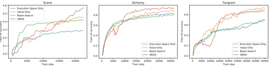
Figure 5: Training hit accuracy on examples with 5 utterances, comparing VBSIX to baselines with ablated components. The results are averaged over 6 runs with different random seeds (best viewed in color)

each component is used separately, when both of them are used (VBSIX), and when none are used (beam-search). We find that both contributions are important for performance, as the full system achieves the highest accuracy in all domains. In SCENE, each component has only a slight advan-tage over beam-search, and therefore both are re-quired to achieve significant improvement. How-ever, in ALCHEMY and TANGRAM most of the gain is due to the value network.

We also directly measured the hit accuracy at training time, i.e., the proportion of training ex-amples where the beam produced by the search al-gorithm contains a program with the correct deno-tation, showing the effectiveness of search at train-ing time. In Figure 5, we report train hit accuracy in each training step, averaged across 6 random seeds. The graphs illustrate the performance of each search algorithm in every domain throughout training. The validation accuracy results are corre-lated with the improvement in train hit-accuracy.

6.3 Analysis

Execution Space We empirically measured two quantities that we expect should reflect the advan-tage of execution-space search. First, we mea-sured the number of programs stored in the execu-tion space graph compared to beam search, which holds K programs. Second, we counted the av-erage number of states that are connected to cor-rect terminal states in the discovered graph, but fell out of the beam during the search. The prop-erty reflects the gain from running search over a graph structure, where the same vertex can resur-face. We preformed the analysis on VBSIX over 5-utterance training examples in all 3 domains. The following table summarizes the results:

We found the measured properties and the con-tribution of execution space in each domain are

Property SCENE ALCHEMY TANGRAM

Paths in beam 143903 5892 678

Correct pruned 18.5 11.2 3.8

correlated, as seen in the ablations. Differences between domains are due to the different com-plexities of their formal languages. As the for-mal language becomes more expressive, the exe-cution space is more compressed as each state can be reached in more ways. In particular, the formal language in SCENEcontains more functions com-pared to the other domains, and so it benefits the most from execution-space search.

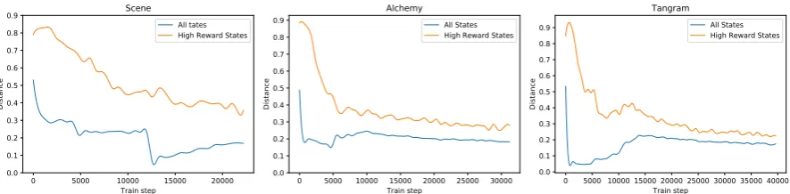
Value Network We analyzed the accuracy of the value network at training time by measuring, for each state, the difference between its expected re-ward (estimated from the discovered paths) and the value network prediction. Figure 6 shows the average difference in each training step for all en-countered states (in blue), and for high reward states only (states with expected reward larger than

0.7, in orange). Those metrics are averaged across

6 runs with different random seeds.

0 5000 10000 15000 20000 Train step

0.0 0.1 0.2 0.3 0.4 0.5 0.6 0.7 0.8 0.9

Distance

Scene

All tates High Reward States

0 5000 10000 15000 20000 25000 30000

Train step 0.0

0.1 0.2 0.3 0.4 0.5 0.6 0.7 0.8 0.9

Distance

Alchemy

All States High Reward States

0 5000 10000 15000 20000 25000 30000 35000 40000

Train step 0.0

0.1 0.2 0.3 0.4 0.5 0.6 0.7 0.8 0.9

Distance

Tangram

All States High Reward States

Figure 6: The difference between the prediction of the value network and the expected reward (estimated from the discovered paths) during training. We report the average difference for all of the states (blue) and for the high reward states only (>0.7, orange). The results are averaged over 6 runs with different random seeds (best viewed in color).

7 Related Work

Training from denotations has been extensively in-vestigated (Kwiatkowski et al., 2013; Pasupat and Liang, 2015; Bisk et al., 2016), with a recent em-phasis on neural models (Neelakantan et al., 2016; Krishnamurthy et al., 2017). Improving beam search has been investigated by proposing special-ized objectives (Wiseman and Rush, 2016), stop-ping criteria (Yang et al., 2018), and using contin-uous relaxations (Goyal et al., 2018).

Bahdanau et al. (2017) and Suhr and Artzi (2018) proposed ways to evaluate intermediate predictions from a sparse reward signal. Bah-danau et al. (2017) used a critic network to es-timate expected BLEU in translation, while Suhr and Artzi (2018) used edit-distance between the current world and the goal for SCONE. But, in those works stronger supervision was assumed: Bahdanau et al. (2017) utilized the gold sequences, and Suhr and Artzi (2018) used intermediate worlds states. Moreover, intermediate evaluations were used to compute gradient updates, rather than for guiding search.

Guiding search with both policy and value networks was done in Monte-Carlo Tree Search (MCTS) for tasks with a sparse reward (Silver et al., 2017; T. A. and and Barber, 2017; Shen et al., 2018). In MCTS, value network evaluations are refined with backup updates to improve policy scores. In this work, we gain this advantage by us-ing the target denotation. The use of an actor and a critic is also reminiscent ofA∗ where states are scored by past cost and an admissible heuristic for future cost (Klein and Manning, 2003; Pauls and Klein, 2009; lee et al., 2016). In semantic parsing, Misra et al. (2018) recently proposed a critic dis-tribution to improve the policy, which is based on

prior domain knowledge (that is not learned).

8 Conclusions

In this work, we propose a new training algorithm for mapping instructions to programs given deno-tation supervision only. Our algorithm exploits the denotation at training time to train a critic network used to rank search states on the beam, and per-forms search in a compact execution space rather than in the space of programs. We evaluated on three different domains from SCONE, and found that it dramatically improves performance com-pared to strong baselines across all domains.

VBSIX is applicable to any task that supports graph-search exploration. Specifically, for tasks that can be formulated as an MDP with a deter-ministic transition function, which allow efficient execution of multiple partial trajectories. Those tasks include a wide range of instruction mapping (Branavan et al., 2009; Vogel and Jurafsky, 2010; Anderson et al., 2018) and semantic parsing tasks (Dahl et al., 1994; Iyyer et al., 2017; Yu et al., 2018). Therefore, evaluating VBSIX on other do-mains is a natural next step for our research.

Acknowledgments

References

P. Anderson, Q. Wu, D. Teney, J. Bruce, M. Johnson, N. S¨underhauf, I. Reid, S. Gould, and A. van den Hengel. 2018. Vision-and-language navigation: In-terpreting visually-grounded navigation instructions in real environments. InComputer Vision and Pat-tern Recognition (CVPR).

Y. Artzi and L. Zettlemoyer. 2013. Weakly supervised learning of semantic parsers for mapping instruc-tions to acinstruc-tions. Transactions of the Association for Computational Linguistics (TACL), 1:49–62.

D. Bahdanau, P. Brakel, K. Xu, A. Goyal, R. Lowe, J. Pineau, A. Courville, and Y. Bengio. 2017. An actor-critic algorithm for sequence prediction. In

International Conference on Learning Representa-tions (ICLR).

J. Berant, A. Chou, R. Frostig, and P. Liang. 2013. Se-mantic parsing on Freebase from question-answer pairs. InEmpirical Methods in Natural Language Processing (EMNLP).

J. Berant and P. Liang. 2015. Imitation learning of agenda-based semantic parsers. Transactions of the Association for Computational Linguistics (TACL), 3:545–558.

Y. Bisk, D. Yuret, and D. Marcu. 2016. Natural language communication with robots. In North American Association for Computational Linguis-tics (NAACL).

S. Branavan, H. Chen, L. S. Zettlemoyer, and R. Barzi-lay. 2009. Reinforcement learning for mapping in-structions to actions. In Association for Compu-tational Linguistics and International Joint Con-ference on Natural Language Processing (ACL-IJCNLP), pages 82–90.

D. L. Chen and R. J. Mooney. 2011. Learning to in-terpret natural language navigation instructions from observations. InAssociation for the Advancement of Artificial Intelligence (AAAI), pages 859–865.

J. Cheng, S. Reddy, V. Saraswat, and M. Lapata. 2017. Learning structured natural language representations for semantic parsing. In Association for Computa-tional Linguistics (ACL).

J. Clarke, D. Goldwasser, M. Chang, and D. Roth. 2010. Driving semantic parsing from the world’s re-sponse. InComputational Natural Language Learn-ing (CoNLL), pages 18–27.

D. A. Dahl, M. Bates, M. Brown, W. Fisher, K. Hunicke-Smith, D. Pallett, C. Pao, A. Rudnicky, and E. Shriberg. 1994. Expanding the scope of the ATIS task: The ATIS-3 corpus. InWorkshop on Hu-man Language Technology, pages 43–48.

H. Daume, J. Langford, and D. Marcu. 2009. Search-based structured prediction. Machine Learning, 75:297–325.

D. Fried, J. Andreas, and D. Klein. 2018. Unified prag-matic models for generating and following instruc-tions. InNorth American Association for Computa-tional Linguistics (NAACL).

O. Goldman, V. Latcinnik, U. Naveh, A. Globerson, and J. Berant. 2018. Weakly-supervised semantic parsing with abstract examples. InAssociation for Computational Linguistics (ACL).

K. Goyal, G. Neubig, C. Dyer, and T. Berg-Kirkpatrick. 2018. A continuous relaxation of beam search for end-to-end training of neural sequence models. In

Association for the Advancement of Artificial Intel-ligence (AAAI).

K. Guu, P. Pasupat, E. Z. Liu, and P. Liang. 2017. From language to programs: Bridging reinforce-ment learning and maximum marginal likelihood. In

Association for Computational Linguistics (ACL).

S. Hochreiter and J. Schmidhuber. 1997. Long short-term memory. Neural Computation, 9(8):1735– 1780.

Mohit Iyyer, Wen-tau Yih, and Ming-Wei Chang. 2017. Search-based neural structured learning for sequen-tial question answering. InProceedings of the 55th Annual Meeting of the Association for Computa-tional Linguistics (Volume 1: Long Papers), vol-ume 1, pages 1821–1831.

D. Kingma and J. Ba. 2014. Adam: A method for stochastic optimization. arXiv preprint arXiv:1412.6980.

D. Klein and C. Manning. 2003. A* parsing: Fast exact viterbi parse selection. InHuman Language Tech-nology and North American Association for Compu-tational Linguistics (HLT/NAACL).

J. Krishnamurthy, P. Dasigi, and M. Gardner. 2017. Neural semantic parsing with type constraints for semi-structured tables. In Empirical Methods in Natural Language Processing (EMNLP).

J. Krishnamurthy and T. Mitchell. 2012. Weakly supervised training of semantic parsers. In Em-pirical Methods in Natural Language Processing and Computational Natural Language Learning (EMNLP/CoNLL), pages 754–765.

T. Kwiatkowski, E. Choi, Y. Artzi, and L. Zettlemoyer. 2013. Scaling semantic parsers with the-fly on-tology matching. InEmpirical Methods in Natural Language Processing (EMNLP).

K. lee, M. Lewis, and L. Zettlemoyer. 2016. Global neural CCG parsing with optimality guarantees. In

Empirical Methods in Natural Language Processing (EMNLP).

C. Liang, J. Berant, Q. Le, and K. D. F. N. Lao. 2017. Neural symbolic machines: Learning seman-tic parsers on Freebase with weak supervision. In

C. Liang, M. Norouzi, J. Berant, Q. Le, and N. Lao. 2018. Memory augmented policy optimization for program synthesis with generalization. InAdvances in Neural Information Processing Systems (NIPS).

P. Liang, M. I. Jordan, and D. Klein. 2011. Learn-ing dependency-based compositional semantics. In

Association for Computational Linguistics (ACL), pages 590–599.

R. Long, P. Pasupat, and P. Liang. 2016. Simpler context-dependent logical forms via model projec-tions. InAssociation for Computational Linguistics (ACL).

Dipendra Misra, Ming-Wei Chang, Xiaodong He, and Wen-tau Yih. 2018. Policy shaping and generalized update equations for semantic parsing from denota-tions. arXiv preprint arXiv:1809.01299.

A. Neelakantan, Q. V. Le, and I. Sutskever. 2016. Neural programmer: Inducing latent programs with gradient descent. In International Conference on Learning Representations (ICLR).

P. Pasupat and P. Liang. 2015. Compositional semantic parsing on semi-structured tables. InAssociation for Computational Linguistics (ACL).

P. Pasupat and P. Liang. 2016. Inferring logical forms from denotations. InAssociation for Computational Linguistics (ACL).

A. Pauls and D. Klein. 2009. K-best A* parsing. In

Association for Computational Linguistics (ACL), pages 958–966.

J. Pennington, R. Socher, and C. D. Manning. 2014. GloVe: Global vectors for word representation. In

Empirical Methods in Natural Language Processing (EMNLP), pages 1532–1543.

M. Rabinovich, M. Stern, and D. Klein. 2017. Abstract syntax networks for code generation and semantic parsing. InAssociation for Computational Linguis-tics (ACL).

S. Ross, G. Gordon, and A. Bagnell. 2011. A reduction of imitation learning and structured prediction to no-regret online learning. InArtificial Intelligence and Statistics (AISTATS).

Y. Shen, J. Chen, P. Huang, Y. Guo, and J. Gao. 2018. Reinforcewalk: Learning to walk in graph with monte carlo tree search. InInternational Con-ference on Learning Representations (ICLR).

D. Silver, J. Schrittwieser, K. Simonyan, I. Antonoglou, A. Huang, A. Guez, T. Hubert, L., M. Lai, A. Bolton, et al. 2017. Mastering the game of go without human knowledge. Nature, 550(7676):354–359.

A. Suhr and Y. Artzi. 2018. Situated mapping of se-quential instructions to actions with single-step re-ward observation. InAssociation for Computational Linguistics (ACL).

I. Sutskever, O. Vinyals, and Q. V. Le. 2014. Sequence to sequence learning with neural networks. In Ad-vances in Neural Information Processing Systems (NIPS), pages 3104–3112.

R. Sutton, D. McAllester, S. Singh, and Y. Mansour. 1999. Policy gradient methods for reinforcement learning with function approximation. InAdvances in Neural Information Processing Systems (NIPS).

Z. Tian T. A. and and D. Barber. 2017. Thinking Fast and Slow with Deep Learning and Tree Search. Ad-vances in Neural Information Processing Systems 30.

A. Vogel and D. Jurafsky. 2010. Learning to follow navigational directions. InAssociation for Compu-tational Linguistics (ACL), pages 806–814.

R. J. Williams. 1992. Simple statistical gradient-following algorithms for connectionist reinforce-ment learning. Machine learning, 8(3):229–256.

S. Wiseman and A. M. Rush. 2016. Sequence-to-sequence learning as beam-search optimization. In

Empirical Methods in Natural Language Processing (EMNLP).

Y. Yang, L. Huang, and M. Ma. 2018. Breaking the beam search curse: A study of (re-) scoring methods and stopping criteria for neural machine translation. InEmpirical Methods in Natural Language Process-ing (EMNLP).

P. Yin and G. Neubig. 2017. A syntactic neural model for general-purpose code generation. InAssociation for Computational Linguistics (ACL), pages 440– 450.

Tao Yu, Rui Zhang, Kai Yang, Michihiro Yasunaga, Dongxu Wang, Zifan Li, James Ma, Irene Li, Qingn-ing Yao, Shanelle Roman, et al. 2018. Spider: A large-scale human-labeled dataset for complex and cross-domain semantic parsing and text-to-sql task.

arXiv preprint arXiv:1809.08887.

A Neural Network Architecture

We adopt the modelπθ(·)proposed by Guu et al.

(2017). The model receives the current utterance

uiand the program stackψ. A bidirectional LSTM (Hochreiter and Schmidhuber, 1997) is used to embed ui, while ψ is embedded by

concatenat-ing the embeddconcatenat-ing of stack elements. The em-bedded input is then fed to a feed-forward net-work with attention over the LSTM hidden states, followed by a softmax layer that predicts a pro-gram token. Our value network Vφ(·) shares the

input layer of πθ(·). In addition, it receives the

next utteranceui+1_{, the current world statew}i_and

BiLSTM ui

𝜓

RelU Att. Softmax z_t

wi

RelU Sigmoid v

wM

ui+1

BiLSTM

Figure 7: The model proposed by Guu et al. (2017) (top), and our value network (bottom).

states are embedded by concatenating embeddings of SCONE elements. The inputs are concatenated and fed to a feed-forward network, followed by a sigmoid layer that outputs a scalar.

B Hyper-parameters

Table 3 contains the hyper-parameter setting for each experiment. Hyper-parameters of REIN-FORCE and MML were taken from Guu et al. (2017). In all experiments learning rate was 0.001 and mini-batch size was 8. We explicitly define the following hyper-parameters which are not self-explanatory:

1. Training steps: The number of training steps taken.

2. Sample size: Number of samples drawn from

pθin REINFORCE

3. Baseline: A constant subtracted from the re-ward for variance reduction.

4. Execution beam size:Kin Algorithm 1. 5. Program bea size: Size of beam in line 3 of Algorithm 1.

6. Value ranking start step: Step when we start ranking states using the critic score.

7. Value re-rank size: Size of beamK0 returned

by the actor score before re-ranking with the actor-critic score.

C Prior Work

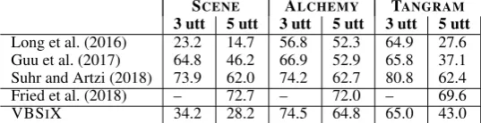
In prior work on SCONE, models were trained on sequences of 1 or 2 utterances, and thus were exposed during training to all gold intermediate states (Long et al., 2016; Guu et al., 2017; Suhr and Artzi, 2018). Fried et al. (2018) assumed

ac-cess to the full annotated logical form. In con-trast, we trained from longer sequences, keeping the logical form and intermediate states latent. We report the test accuracy as reported by prior work and in this paper, noting that our results are an av-erage of 6 runs, while prior work reports the me-dian of 5 runs.

Naturally, our results are lower compared to prior work that uses much stronger supervision. This is because our setup poses a hard search prob-lem at training time, and also requires overcom-ingspuriousness– the fact that even incorrect pro-grams sometimes lead to high reward.

D Value Network Analysis

We analyzed the ability of the value network to predict expected reward. The reward of a state de-pends on two properties, (a)connectivity: whether there is a trajectory from this state to a correct ter-minal state, and (b)model likelihood: the proba-bility the model assigns to those trajectories. We collected a random set of 120 states in the SCENE domain from, where the real expected reward was very high (> 0.7), or very low(= 0.0) and the value network predicted well (less than0.2 devia-tion) or poorly (more than0.5deviation). For ease of analysis we only look at states from the final utterance.

To analyze connectivity, we looked at states that cannot reach a correct terminal state with a single action (since states in the last utterance can per-form one action only, the expected reward is 0). Those are states where either their current and tar-get world differ in too many ways, or the stack content is not relevant to the differences between the worlds. We find that when there are many dif-ferences between the current and target world, the value network correctly estimates low expected re-ward in87.0%of the cases. However, when there is just one mismatch between the current and tar-get world, the value network tends to ignore it and erroneously predicts high reward in 78.9% of the cases.

System SCENE ALCHEMY TANGRAM

REINFORCE Training steps= 22.5k Training steps= 31.5k Training steps= 40k

Sample size= 32 Sample size= 32 Sample size= 32

= 0.2 = 0.2 = 0.2

Baseline= 10−5 Baseline= 10−2 Baseline= 10−3

MML Training steps= 22.5k Training steps= 31.5k Training steps= 40k

Beam size= 32 Beam size= 32 Beam size= 32

= 0.15 = 0.15 = 0.15

VBSiX Training steps= 22.5k Training steps= 31.5k Training steps= 40k

Execution beam size= 32 Execution beam size= 32 Execution beam size= 32

Program beam size= 8 Program beam= 8 Program beam size= 8

= 0.15 = 0.15 = 0.15

Value ranking start step= 5k Value ranking start step= 5k Value ranking start step= 10k

Value re-rank size= 128 Value re-rank size= 128 Value re-rank size= 128

Table 3: Hyper-parameter settings.

SCENE ALCHEMY TANGRAM

3 utt 5 utt 3 utt 5 utt 3 utt 5 utt

Long et al. (2016) 23.2 14.7 56.8 52.3 64.9 27.6

Guu et al. (2017) 64.8 46.2 66.9 52.9 65.8 37.1

Suhr and Artzi (2018) 73.9 62.0 74.2 62.7 80.8 62.4

Fried et al. (2018) – 72.7 – 72.0 – 69.6

VBSIX 34.2 28.2 74.5 64.8 65.0 43.0

Table 4: Test accuracy comparison to prior work.