A Boosting Algorithm for Classification of Semi Structured Text

A Boosting Algorithm for Classification of Semi-Structured Text

Taku Kudo∗ Yuji Matsumoto

Graduate School of Information Science, Nara Institute of Science and Technology

8916-5 Takayama, Ikoma Nara Japan {taku-ku,matsu}@is.naist.jp

Abstract

The focus of research in text classification has ex-panded from simple topic identification to more challenging tasks such as opinion/modality identi-fication. Unfortunately, the latter goals exceed the ability of the traditional bag-of-word representation approach, and a richer, more structural representa-tion is required. Accordingly, learning algorithms must be created that can handle the structures ob-served in texts. In this paper, we propose a Boosting algorithm that captures sub-structures embedded in texts. The proposal consists of i) decision stumps that use subtrees as features and ii) the Boosting al-gorithm which employs the subtree-based decision stumps as weak learners. We also discuss the rela-tion between our algorithm and SVMs with tree ker-nel. Two experiments on opinion/modality classifi-cation confirm that subtree features are important.

1 Introduction

Text classification plays an important role in orga-nizing the online texts available on the World Wide Web, Internet news, and E-mails. Until recently, a number of machine learning algorithms have been applied to this problem and have been proven suc-cessful in many domains (Sebastiani, 2002).

In the traditional text classification tasks, one has to identify predefined text “topics”, such as politics, finance, sports or entertainment. For learning algo-rithms to identify these topics, a text is usually rep-resented as a bag-of-words, where a text is regarded as a multi-set (i.e., a bag) of words and the word or-der or syntactic relations appearing in the original text is ignored. Even though the bag-of-words rep-resentation is naive and does not convey the mean-ing of the original text, reasonable accuracy can be obtained. This is because each word occurring in the text is highly relevant to the predefined “topics” to be identified.

∗

At present, NTT Communication Science Laboratories, 2-4, Hikaridai, Seika-cho, Soraku, Kyoto, 619-0237 Japan [email protected]

Given that a number of successes have been re-ported in the field of traditional text classification, the focus of recent research has expanded from sim-ple topic identification to more challenging tasks such as opinion/modality identification. Example includes categorization of customer E-mails and re-views by types of claims, modalities or subjectiv-ities (Turney, 2002; Wiebe, 2000). For the lat-ter, the traditional bag-of-words representation is not sufficient, and a richer, structural representa-tion is required. A straightforward way to ex-tend the traditional bag-of-words representation is to heuristically add new types of features to the original bag-of-words features, such as fixed-length n-grams (e.g., word bi-gram or tri-gram) or fixed-length syntactic relations (e.g., modifier-head rela-tions). These ad-hoc solutions might give us rea-sonable performance, however, they are highly task-dependent and require careful design to create the “optimal” feature set for each task.

Generally speaking, by using text processing sys-tems, a text can be converted into a semi-structured text annotated with parts-of-speech, base-phrase in-formation or syntactic relations. This inin-formation is useful in identifying opinions or modalities con-tained in the text. We think that it is more useful to propose a learning algorithm that can automatically capture relevant structural information observed in text, rather than to heuristically add this informa-tion as new features. From these points of view, this paper proposes a classification algorithm that cap-tures sub-struccap-tures embedded in text. To simplify the problem, we first assume that a text to be classi-fied is represented as a labeled ordered tree, which is a general data structure and a simple abstraction of text. Note that word sequence, base-phrase anno-tation, dependency tree and an XML document can be modeled as a labeled ordered tree.

of the candidate feature set becomes quite large, it automatically selects a compact and relevant feature set based on Boosting.

This paper is organized as follows. First, we describe the details of our Boosting algorithm in which the subtree-based decision stumps are ap-plied as weak learners. Second, we show an imple-mentation issue related to constructing an efficient learning algorithm. We also discuss the relation be-tween our algorithm and SVMs (Boser et al., 1992) with tree kernel (Collins and Duffy, 2002; Kashima and Koyanagi, 2002). Two experiments on the opin-ion and modality classificatopin-ion tasks are employed to confirm that subtree features are important.

2 Classifier for Trees

We first assume that a text to be classified is repre-sented as a labeled ordered tree. The focused prob-lem can be formalized as a general probprob-lem, called the tree classification problem.

The tree classification problem is to induce a mapping f(x) : X → {±1}, from given training examples T = {hxi, yii}Li=1, where xi ∈ X is a labeled ordered tree andyi ∈ {±1}is a class label associated with each training data (we focus here on the problem of binary classification.). The im-portant characteristic is that the input examplexi is represented not as a numerical feature vector (bag-of-words) but a labeled ordered tree.

2.1 Preliminaries

Let us introduce a labeled ordered tree (or simply tree), its definition and notations, first.

Definition 1 Labeled ordered tree (Tree)

A labeled ordered tree is a tree where each node is associated with a label and is ordered among its siblings, that is, there are a first child, second child, third child, etc.

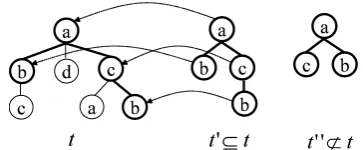
Definition 2 Subtree

Let tandu be labeled ordered trees. We say that t matches u, or t is a subtree of u (t ⊆ u), if there exists a one-to-one function ψ from nodes in ttou, satisfying the conditions: (1)ψpreserves the parent-daughter relation, (2) ψ preserves the sib-ling relation, (3)ψpreserves the labels.

We denote the number of nodes intas|t|. Figure 1 shows an example of a labeled ordered tree and its subtree and non-subtree.

2.2 Decision Stumps

Decision stumps are simple classifiers, where the final decision is made by only a single hypothesis

Figure 1: Labeled ordered tree and subtree relation

or feature. Boostexter (Schapire and Singer, 2000) uses word-based decision stumps for topic-based text classification. To classify trees, we here extend the decision stump definition as follows.

Definition 3 Decision Stumps for Trees

Let t and x be labeled ordered trees, and y be a class label (y ∈ {±1}), a decision stump classifier for trees is given by

h_ht,yi(x)def=

y t⊆x −y otherwise.

The parameter for classification is the tupleht, yi, hereafter referred to as the rule of the decision stumps.

The decision stumps are trained to find rulehˆt,yiˆ

that minimizes the error rate for the given training dataT ={hxi, yii}Li=1:

hˆt,yˆi = argmin

t∈F,y∈{±1}

1 2L

L X

i=1

(1−yihht,yi(xi)),(1)

whereF is a set of candidate trees or a feature set (i.e.,F =SL_i=1{t|t⊆xi}).

The gain function for ruleht, yiis defined as

gain(ht, yi)def=

L

X

i=1

yihht,yi(xi). (2)

Using the gain, the search problem given in (1) becomes equivalent to the following problem:

hˆt,yiˆ = argmax

t∈F,y∈{±1}

gain(ht, yi).

In this paper, we will use gain instead of error rate for clarity.

2.3 Applying Boosting

A weak learner is built at each iteration k with different distributions or weights d(k) =

(d(_ik), . . . , d(_Lk)), (whereP_iN₌₁d(_ik) = 1, d(_ik) ≥ 0). The weights are calculated in such a way that hard examples are focused on more than easier examples. To use the decision stumps as the weak learner of Boosting, we redefine the gain function (2) as fol-lows:

gain(ht, yi)def=

L

X

i=1

yidihht,yi(xi). (3)

There exist many Boosting algorithm variants, however, the original and the best known algorithm is AdaBoost (Freund and Schapire, 1996). We here use Arc-GV (Breiman, 1999) instead of AdaBoost, since Arc-GV asymptotically maximizes the margin and shows faster convergence to the optimal solu-tion than AdaBoost.

3 Efficient Computation

In this section, we introduce an efficient and prac-tical algorithm to find the optimal rulehˆt,yiˆ from given training data. This problem is formally de-fined as follows.

Problem 1 Find Optimal Rule

LetT = {hx1, y1, d1i, . . . ,hxL, yL, dLi}be train-ing data, where, xi is a labeled ordered tree, yi ∈ {±1} is a class label associated with xi and di (

P_L

i=1di = 1, di ≥ 0) is a

normal-ized weight assigned to xi. Given T, find the optimal rule ht,ˆyiˆ that maximizes the gain, i.e., ht,ˆyiˆ = argmax_{t∈F,y∈{±1}}diyihht,yi, where F = S_L

i=1{t|t⊆xi}.

The most naive and exhaustive method, in which we first enumerate all subtrees F and then calcu-late the gains for all subtrees, is usually impractical, since the number of subtrees is exponential to its size. We thus adopt an alternative strategy to avoid such exhaustive enumeration.

The method to find the optimal rule is modeled as a variant of the branch-and-bound algorithm, and is summarized in the following strategies:

1. Define a canonical search space in which a whole set of subtrees of a set of trees can be enumerated.

2. Find the optimal rule by traversing this search space.

3. Prune search space by proposing a criterion with respect to the upper bound of the gain.

We will describe these steps more precisely in the following subsections.

3.1 Efficient Enumeration of Trees

Abe and Zaki independently proposed an efficient method, rightmost-extension, to enumerate all sub-trees from a given tree (Abe et al., 2002; Zaki, 2002). First, the algorithm starts with a set of trees consisting of single nodes, and then expands a given tree of size(k−1)by attaching a new node to this tree to obtain trees of size k. However, it would be inefficient to expand nodes at arbitrary positions of the tree, as duplicated enumeration is inevitable. The algorithm, rightmost extension, avoids such du-plicated enumerations by restricting the position of attachment. We here give the definition of rightmost extension to describe this restriction in detail.

Definition 4 Rightmost Extension (Abe et al., 2002;

Zaki, 2002)

Lettandt0 be labeled ordered trees. We sayt0is a rightmost extension oft, if and only iftandt0satisfy the following three conditions:

(1)t0 is created by adding a single node tot, (i.e., t⊂t0_{and|t|+ 1 =|t}0_|).

(2) A node is added to a node existing on the unique path from the root to the rightmost leaf (rightmost-path) int.

(3) A node is added as the rightmost sibling.

Consider Figure 2, which illustrates example treet with the labels drawn from the setL = {a, b, c}. For the sake of convenience, each node in this figure has its original number (depth-first enumeration). The rightmost-path of the tree t is (a(c(b))), and occurs at positions1,4and6respectively. The set of rightmost extended trees is then enumerated by simply adding a single node to a node on the most path. Since there are three nodes on the right-most path and the size of the label set is 3(= |L|), a total of 9 trees are enumerated from the original treet. Note that rightmost extension preserves the prefix ordering of nodes in t (i.e., nodes at posi-tions1..|t|are preserved). By repeating the process of rightmost-extension recursively, we can create a search space in which all trees drawn from the setL are enumerated. Figure 3 shows a snapshot of such a search space.

3.2 Upper bound of gain

b a c 1 2 4 a b 5 6 c 3 b a c 1 2 4 a b 5 6 c 3 b a c 1 2 4 a b 5 6 c 3 b a c 1 2 4 a b 5 6 c 3 rightmost- path t rightmost extension 7 7 7 t’ } , , {abc L=

} , , {abc

} , , {abc

} , , {abc

Figure 2: Rightmost extension

Figure 3: Recursion using rightmost extension

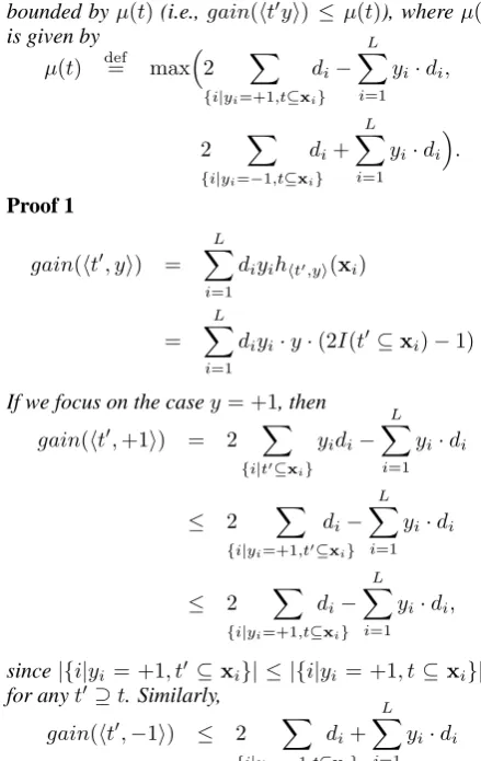
this canonical search space. The following theo-rem, an extension of Morhishita (Morhishita, 2002), gives a convenient way of computing a tight upper bound ongain(ht0, yi)for any super-treet0 oft.

Theorem 1 Upper bound of the gain:µ(t)

For any t0 _{⊇tandy ∈ {±1}, the gain of ht}0_{, yiis} bounded byµ(t)(i.e.,gain(ht0_{yi) ≤µ(t)), whereµ(t)} is given by

µ(t) def= max2 X

{i|yi=+1,t⊆xi}

di− L X

i=1 yi·di,

2 X

{i|yi=−1,t⊆xi}

di+ L X

i=1 yi·di

.

Proof 1

gain(ht0_{, yi) =} L X

i=1

diyihht0_,yi(x_i)

=

L X

i=1

diyi·y·(2I(t0⊆xi)−1)

If we focus on the casey= +1, then

gain(ht0,+1i) = 2 X

{i|t0_⊆x

i}

yidi− L X

i=1 yi·di

≤ 2 X

{i|yi=+1,t0⊆xi}

di− L X

i=1 yi·di

≤ 2 X

{i|yi=+1,t⊆xi}

di− L X

i=1 yi·di,

since|{i|yi = +1, t0 ⊆xi}| ≤ |{i|yi = +1, t⊆xi}| for anyt0_{⊇t. Similarly,}

gain(ht0,−1i) ≤ 2 X

{i|yi=−1,t⊆xi}

di+ L X

i=1 yi·di

Thus, for anyt0_{⊇tandy∈ {±1},}

gain(ht0_{, yi)≤µ(t) 2}

We can efficiently prune the search space spanned by right most extension using the upper bound of gain u(t). During the traverse of the subtree lat-tice built by the recursive process of rightmost ex-tension, we always maintain the temporally subop-timal gainτ among all gains calculated previously. Ifµ(t) < τ, the gain of any super-treet0 ⊇tis no greater thanτ, and therefore we can safely prune the search space spanned from the subtree t. If µ(t) ≥ τ, in contrast, we cannot prune this space, since there might exist a super-tree t0 _{⊇ t such} thatgain(t0) ≥ τ. We can also prune the space with respect to the expanded single node s. Even ifµ(t) ≥ τ and a nodesis attached to the treet, we can ignore the space spanned from the treet0 if µ(s)< τ, since no super-tree ofscan yield optimal gain.

Figure 4 presents a pseudo code of the algorithm

Find Optimal Rule. The two pruning are marked

with (1) and (2) respectively.

4 Relation to SVMs with Tree Kernel

Recent studies (Breiman, 1999; Schapire et al., 1997; R¨atsch et al., 2001) have shown that both Boosting and SVMs (Boser et al., 1992) have a similar strategy; constructing an optimal hypothe-sis that maximizes the smallest margin between the positive and negative examples. We here describe a connection between our Boosting algorithm and SVMs with tree kernel (Collins and Duffy, 2002; Kashima and Koyanagi, 2002).

Tree kernel is one of the convolution kernels, and implicitly maps the example represented in a la-beled ordered tree into all subtree spaces. The im-plicit mapping defined by tree kernel is given as:

Φ(x)=(I(t1 ⊆x), . . . , I(t|F| ⊆x)), wheretj∈F, x∈ X andI(·)is the indicator function1.

The final hypothesis of SVMs with tree kernel can be given by

f(x) = sgn(w·Φ(x)−b) = sgn(X

t∈F

wt·I(t⊆x)−b). (4)

Similarly, the final hypothesis of our boosting al-gorithm can be reformulated as a linear classifier:

1

Algorithm: Find Optimal Rule

argument: T ={hx1, y1, d1i. . . ,hxL, yL, dLi} (xia tree,yi ∈ {±1}is a class, and di (

P_L

i=1di= 1, di ≥0)is a weight) returns: Optimal rulehˆt,yiˆ

begin

τ = 0 // suboptimal value

function project(t)

ifµ(t)≤τ then return . . .(1)

y0 _=argmax

y∈{±1}gain(ht, yi) ifgain(ht, y0i)> τ then

hˆt,yiˆ =ht, y0_i

τ =gain(ht,ˆyiˆ ) // suboptimal solution

end

foreacht0∈ {set of trees that are

rightmost extension oft} s=single node added by RME

ifµ(s)≤τ then continue. . .(2) project(t0)

end end

// for each single node

foreacht0∈ {t|t∈ ∪L_i=1{t|t⊆xi)}, |t|= 1}

project(t0) end

returnhˆt,yiˆ end

Figure 4: Algorithm: Find Optimal Rule

f(x) = sgn(

K X

k=1

αkhhtk,yki(x))

= sgn(

K X

k=1

αk·yk(2I(tk⊆x)−1))

= sgn(X

t∈F

wt·I(t⊆x)−b), (5)

where

b=

K X

k=1

ykαk, wt= X

{k|t=tk}

2·yk·αk.

We can thus see that both algorithms are essentially the same in terms of their feature space. The dif-ference between them is the metric of margin; the margin of Boosting is measured inl1-norm, while,

that of SVMs is measured inl2-norm. The question

one might ask is how the difference is expressed in practice. The difference between them can be ex-plained by sparseness.

It is well known that the solution or separating hyperplane of SVMs is expressed as a linear com-bination of the training examples using some coeffi-cientsλ, (i.e.,w=PL_i=1λiΦ(xi)). Maximizingl2

-norm margin gives a sparse solution in the example space, (i.e., most ofλi becomes0). Examples that have non-zero coefficient are called support vectors that form the final solution. Boosting, in contrast, performs the computation explicitly in the feature space. The concept behind Boosting is that only a few hypotheses are needed to express the final so-lution. Thel1-norm margin allows us to realize this

property. Boosting thus finds a sparse solution in the feature space.

The accuracies of these two methods depends on the given training data. However, we argue that Boosting has the following practical advantages. First, sparse hypotheses allow us to build an effi-cient classification algorithm. The complexity of SVMs with tree kernel isO(L0|N1||N2|), whereN1

and N2 are trees, andL0 is the number of support

vectors, which is too heavy to realize real applica-tions. Boosting, in contrast, runs faster, since the complexity depends only on the small number of de-cision stumps. Second, sparse hypotheses are use-ful in practice as they provide “transparent” models with which we can analyze how the model performs or what kind of features are useful. It is difficult to give such analysis with kernel methods, since they define the feature space implicitly.

5 Experiments

5.1 Experimental Setting

We conducted two experiments in sentence classifi-cation.

• PHS review classification (PHS)

The goal of this task is to classify reviews (in Japanese) for PHS2as positive reviews or neg-ative reviews. A total of 5,741 sentences were collected from a Web-based discussion BBS on PHS, in which users are directed to submit positive reviews separately from negative re-views. The unit of classification is a sentence. The categories to be identified are “positive” or “negative” with the numbers 2,679 and 3,062 respectively.

• Modality identification (MOD)

This task is to classify sentences (in Japanese) by modality. A total of 1,710 sentences from a Japanese newspaper were manually annotated

2_{PHS (Personal Handyphone System) is a cell phone}

according to Tamura’s taxonomy (Tamura and Wada, 1996). The unit of classification is a sentence. The categories to be identified are “opinion”, “assertion” or “description” with the numbers 159, 540, and 1,011 respectively.

To employ learning and classification, we have to represent a given sentence as a labeled ordered tree. In this paper, we use the following three representa-tion forms.

• bag-of-words (bow), baseline

Ignoring structural information embedded in text, we simply represent a text as a set of words. This is exactly the same setting as Boostexter. Word boundaries are identi-fied using a Japanese morphological analyzer, ChaSen3.

• Dependency (dep)

We represent a text in a word-based depen-dency tree. We first use CaboCha4to obtain a chunk-based dependency tree of the text. The chunk approximately corresponds to the base-phrase in English. By identifying the head word in the chunk, a chunk-based dependency tree is converted into a word-based dependency tree.

• N-gram (ngram)

It is the word-based dependency tree that as-sumes that each word simply modifies the next word. Any subtree of this structure becomes a word n-gram.

We compared the performance of our Boosting al-gorithm and support vector machines (SVMs) with bag-of-words kernel and tree kernel according to their F-measure in 5-fold cross validation. Although there exist some extensions for tree kernel (Kashima and Koyanagi, 2002), we use the original tree ker-nel by Collins (Collins and Duffy, 2002), where all subtrees of a tree are used as distinct features. This setting yields a fair comparison in terms of feature space. To extend a binary classifier to a multi-class classifier, we use the one-vs-rest method. Hyperpa-rameters, such as number of iterationsKin Boost-ing and soft-margin parameterCin SVMs were se-lected by using cross-validation. We implemented SVMs with tree kernel based on TinySVM5 with custom kernels incorporated therein.

3

http://chasen.naist.jp/

4_{http://chasen.naist.jp/˜ taku/software/cabocha/} 5

http://chasen.naist.jp/˜ taku/software/tinysvm

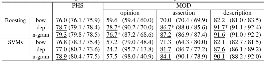
5.2 Results and Discussion

Table 1 summarizes the results of PHS and MOD tasks. To examine the statistical significance of the results, we employed a McNemar’s paired test, a variant of the sign test, on the labeling disagree-ments. This table also includes the results of sig-nificance tests.

5.2.1 Effects of structural information

In all tasks and categories, our subtree-based Boost-ing algorithm (dep/ngram) performs better than the baseline method (bow). This result supports our first intuition that structural information within texts is important when classifying a text by opinions or modalities, not by topics. We also find that there are no significant differences in accuracy between dependency and n-gram (in all cases,p >0.2).

5.2.2 Comparison with Tree Kernel

When using the bag-of-words feature, no signifi-cant differences in accuracy are observed between Boosting and SVMs. When structural information is used in training and classification, Boosting per-forms slightly better than SVMs with tree kernel. The differences are significant when we use de-pendency features in the MOD task. SVMs show worse performance depending on tasks and gories, (e.g., 24.2 F-measure in the smallest cate-gory “opinion” in the MOD task).

Table 1: Results of Experiments on PHS / MOD, F-measure, precision (%), and recall (%)

PHS MOD

opinion assertion description

Boosting bow 76.0 (76.1 / 75.9) 59.6 (59.4 / 60.0) 70.0 (70.4 / 69.9) 82.2 (81.0 / 83.5)

dep 78.7 (79.1 / 78.4) 78.7* (90.2 / 70.0) 86.7* (88.0 / 85.6) 91.7* (91.1 / 92.4)

n-gram 79.3 (79.8 / 78.5) 76.7* (87.2 / 68.6) 87.2 (86.9 / 87.4) 91.6 (91.0 / 92.2)

SVMs bow 76.8 (78.3 / 75.4) 57.2 (79.0 / 48.4) 71.3 (64.3 / 80.0) 82.1 (82.7 / 81.5)

dep 77.0 (80.7 / 73.6) 24.2 (95.7 / 13.8) 81.7 (86.7 / 77.2) 87.6 (86.1 / 89.2)

n-gram 78.9 (80.4 / 77.5) 57.5 (98.0 / 40.9) 84.1 (90.1 / 78.9) 90.1 (88.2 / 92.0)

We employed a McNemar’s paired test on the labeling disagreements. Underlined results indicate that there is a significant differ-ence (p < 0.01) against the baseline (bow). If there is a statistical difference (p < 0.01) between Boosting and SVMs with the same feature representation (bow / dep / n-gram), better results are asterisked.

5.2.3 Merits of our algorithm

In the previous section, we described the merits of our Boosting algorithm. We experimentally verified these merits from the results of the PHS task.

As illustrated in section 4, our method can auto-matically select relevant and compact features from a number of feature candidates. In the PHS task, a total 1,793 features (rules) were selected, while the set sizes of distinct uni-gram, bi-gram and tri-gram appearing in the data were 4,211, 24,206, and 43,658 respectively. Even though all subtrees are used as feature candidates, Boosting selects a small and highly relevant subset of features. When we explicitly enumerate the subtrees used in tree ker-nel, the number of active (non-zero) features might amount to ten thousand or more.

Table 2 shows examples of extracted support fea-tures (pairs of feature (tree)tand weightwtin (Eq. 5)) in the PHS task.

A. Features including the word “にくい(hard, dif-ficult)”

In general, “にくい(hard, difficult)” is an ad-jective expressing negative opinions. Most of features including “に くい” are assigned a negative weight (negative opinion). How-ever, only one feature “切れに くい (hard to cut off)” has a positive weight. This result strongly reflects the domain knowledge, PHS (cell phone reviews).

B. Features including the word “使う(use)” “使う(use)” is a neutral expression for opin-ion classificatopin-ions. However, the weight varies according to the surrounding context: 1) “使い たい(want to use)”→positive, 2) “使い やす い(be easy to use)”→positive, 3) “使い やす か った(was easy to use)” (past form)→ neg-ative, 4) “の ほうが 使い やすい(... is easier to use than ..)” (comparative)→negative.

C. Features including the word “充電(recharge)” Features reflecting the domain knowledge are

Table 2: Examples of features in PHS dataset keyword wtsubtreet(support features)

A.にくい 0.0004切れる にくい(be hard to cut off)

(hard, -0.0006読む にくい(be hard to read)

difficult) -0.0007使う にくい(be hard to use)

-0.0017にくい(be hard to)

B.使う 0.0027使う たい(want to use)

(use) 0.0002使う(use)

0.0002使う てる(be in use)

0.0001使う やすい(be easy to use)

-0.0001使う やすい た(was easy to use)

-0.0007使う にくい(be hard to use)

-0.0019方 が 使う やすい(is easier to use than)

C.充電 0.0028充電 時間 が 短い(recharging time is short)

(recharge) -0.0041充電 時間 が 長い(recharging time is long)

extracted: 1) “充電 時間 が 短い(recharging time is short)” → positive, 2) “充電 時間 が

長い (recharging time is long)” → negative. These features are interesting, since we cannot determine the correct label (positive/negative) by using just the bag-of-words features, such as “recharge”, “short” or “long” alone.

Table 3 illustrates an example of actual classifica-tion. For the input sentence “液晶が大きくて,綺麗,

見やすい(The LCD is large, beautiful, and easy to see.)”, the system outputs the features applied to this classification along with their weightswt. This in-formation allows us to analyze how the system clas-sifies the input sentence in a category and what kind of features are used in the classification. We can-not perform these analyses with tree kernel, since it defines their feature space implicitly.

The testing speed of our Boosting algorithm is much higher than that of SVMs with tree kernel. In the PHS task, the speeds of Boosting and SVMs are 0.531 sec./5,741 instances and 255.42 sec./5,741 in-stances respectively6. We can say that Boosting is

6_{We ran these tests on a Linux PC with XEON 2.4Ghz dual}

Table 3: A running example Input:液晶が大きくて綺麗,見やすい. The LCD is large, beautiful and easy to see.

w_t subtreet(support features)

0.00368 やすい(be easy to)

0.00352 綺麗(beautiful)

0.00237 見る やすい(be easy to see)

0.00174 が 大きい(... is large)

0.00107 液晶 が 大きい(The LCD is large)

0.00074 液晶 が(The LCD is ...)

0.00058 液晶(The LCD)

0.00027 て(a particle for coordination)

0.00036 見る(see)

-0.00001 大きい(large)

-0.00052 が(a nominative case marker)

about 480 times faster than SVMs with tree kernel. Even though the potential size of search space is huge, the pruning criterion proposed in this pa-per effectively prunes the search space. The prun-ing conditions in Fig.4 are fulfilled with more than 90% probabitity. The training speed of our method is 1,384 sec./5,741 instances when we set K =

60,000 (# of iterations for Boosting). It takes only 0.023(=1,384/60,000)sec. to invoke the weak learner, Find Optimal Rule.

6 Conclusions and Future Work

In this paper, we focused on an algorithm for the classification of semi-structured text in which a sen-tence is represented as a labeled ordered tree7. Our proposal consists of i) decision stumps that use subtrees as features and ii) Boosting algorithm in which the subtree-based decision stumps are ap-plied as weak learners. Two experiments on opin-ion/modality classification tasks confirmed that sub-tree features are important.

One natural extension is to adopt confidence rated predictions to the subtree-based weak learners. This extension is also found in BoosTexter and shows better performance than binary-valued learners.

In our experiments, n-gram features showed com-parable performance to dependency features. We would like to apply our method to other applications where instances are represented in a tree and their subtrees play an important role in classifications (e.g., parse re-ranking (Collins and Duffy, 2002) and information extraction).

References

Kenji Abe, Shinji Kawasoe, Tatsuya Asai, Hiroki Arimura, and Setsuo Arikawa. 2002. Optimized

7_{An implementation of our Boosting algorithm is available}

at http://chasen.org/˜ taku/software/bact/

substructure discovery for semi-structured data. In Proc. of PKDD, pages 1–14.

Bernhard Boser, Isabelle Guyon, and Vladimir Vap-nik. 1992. A training algorithm for optimal mar-gin classifiers. In In Proc of 5th COLT, pages 144–152.

Leo Breiman. 1999. Prediction games and arch-ing algoritms. Neural Computation, 11(7):1493 – 1518.

Michael Collins and Nigel Duffy. 2002. New rank-ing algorithms for parsrank-ing and taggrank-ing: Kernels over discrete structures, and the voted perceptron. In Proc. of ACL.

Yoav Freund and Robert E. Schapire. 1996. A decision-theoretic generalization of on-line learn-ing and an application to boostlearn-ing. Journal of Computer and System Sicences, 55(1):119–139. David Haussler. 1999. Convolution kernels on

dis-crete structures. Technical report, UC Santa Cruz (UCS-CRL-99-10).

Hisashi Kashima and Teruo Koyanagi. 2002. Svm kernels for semi-structured data. In Proc. of ICML, pages 291–298.

Shinichi Morhishita. 2002. Computing optimal hy-potheses efficiently for boosting. In Progress in Discovery Science, pages 471–481. Springer. Gunnar. R¨atsch, Takashi. Onoda, and Klaus-Robert

M¨uller. 2001. Soft margins for AdaBoost. Ma-chine Learning, 42(3):287–320.

Robert E. Schapire and Yoram Singer. 2000. Boos-Texter: A boosting-based system for text catego-rization. Machine Learning, 39(2/3):135–168. Robert E. Schapire, Yoav Freund, Peter Bartlett, and

Wee Sun Lee. 1997. Boosting the margin: a new explanation for the effectiveness of voting meth-ods. In Proc. of ICML, pages 322–330.

Fabrizio Sebastiani. 2002. Machine learning in automated text categorization. ACM Computing Surveys, 34(1):1–47.

Naoyoshi Tamura and Keiji Wada. 1996. Text structuring by composition and decomposition of segments (in Japanese). Journal of Natural Lan-guage Processing, 5(1).

Peter D. Turney. 2002. Thumbs up or thumbs down? semantic orientation applied to unsuper-vised classification of reviews. In Proc. of ACL, pages 417–424.

Janyce M. Wiebe. 2000. Learning subjective adjec-tives from corpora. In Proc. of AAAI/IAAI, pages 735–740.