Learning Sequence Encoders for Temporal Knowledge Graph Completion

4816

Learning Sequence Encoders for Temporal Knowledge Graph Completion

Alberto Garc´ıa-Dur´an1 _{Sebastijan Dumanˇci´c}∗2 _{Mathias Niepert}1

1_{NEC Labs Europe, Germany}

{alberto.duran, mathias.niepert}@neclab.eu

2_{KU Leuven, Belgium}

sebastijan.dumancic@cs.kuleuven.be

Abstract

Research on link prediction in knowledge graphs has mainly focused on static multi-relational data. In this work we consider tem-poral knowledge graphs where relations be-tween entities may only hold for a time in-terval or a specific point in time. In line with previous work on static knowledge graphs, we propose to address this problem by learning latent entity and relation type representations. To incorporate temporal information, we uti-lize recurrent neural networks to learn time-aware representations of relation types which can be used in conjunction with existing latent factorization methods. The proposed approach is shown to be robust to common challenges in real-world KGs: the sparsity and hetero-geneity of temporal expressions. Experiments show the benefits of our approach on four tem-poral KGs. The data sets are available under a permissive BSD-3 license1_.

1 Introduction

Knowledge graphs (KGs) are used to organize, manage, and retrieve structured information. The incompleteness of most real-world KGs has stim-ulated research on predicting missing relations be-tween entities. A KG is of the formG = (E, R), whereE is a set of entities and,R is a set of re-lation types or predicates. One can represent G

as a set of triples of the form (subject, predicate, object), denoted as(s,p,o). The link prediction problem seeks the most probable completion of a triple (s,p,?) or(?,p,o) (Nickel et al., 2016). We focus on temporal KGs where some triples are augmented with time information and the link pre-diction problem asks for the most probable com-pletion given time information. More formally, a temporal KG G = (E, R, T) is a KG where

∗

Work done while interning at NEC Labs Europe

1_{https://github.com/nle-ml/mmkb}

facts can also have the form (subject, predicate, object, timestamp) or (subject, predicate, object, time predicate, timestamp), in addition to(s,p,o)

triples. For instance, facts such as (Barack Obama, born, US, 1961) or (Barack Obama, president, US, occursSince, 2009-01) express temporal in-formation about the facts associated with Barack Obama. While the former expresses that a relation type occurred at a specific point in time, the latter expresses an (open) time interval using the time predicate “occursSince.” The latter example also illustrates a common challenge posed by the het-erogeneity of time expressions due to variations in language and serialization standards.

2 Related Work

Reasoning with temporal information in knowl-edge bases has a long history and has resulted in numerous temporal logics (van Benthem, 1995). Several recent approaches extend statistical rela-tional learning frameworks with temporal reason-ing capabilities (Chekol et al., 2017;Chekol and Stuckenschmidt,2018;Dylla et al.,2013).

There is also prior work on incorporating tem-poral information in knowledge graph completion methods. Jiang et al. (2016) capture the temporal ordering that exists between some relation types as well as additional common-sense constraints to generate more accurate link predictions. Es-teban et al. (2016) introduce a prediction model for link prediction that assumes that changes to a KG are introduced by incoming events. These events are modeled as a separate event graph and used to predict the existence of links in the future.

Trivedi et al. (2017) model the occurrence of a fact as a point process whose intensity function is influenced by the score assigned to the fact by an embedding function. Leblay and Chekol (2018) develop scoring functions that incorporate time representations into a TransE-type scoring func-tion. Prior work has also incorporated numeri-cal but non-temporal entity information for knowl-edge base completion (Garcia-Duran and Niepert,

2017).

Contrary to all previous approaches, we encode sequences of temporal tokens with an RNN. This facilitates the encoding of relation types with tem-poral tokens such as “since,” ”until,” and the dig-its of timestamps. Moreover, the RNN encoding provides an inductive bias for parameter sharing among similar timestamps (e.g., those occurring in the same century). Finally, our method can be combined with all existing scoring functions.

3 Time-Aware Representations

Embedding approaches for KG completion learn a scoring functionf that operates on the embed-dings of the subjectes, the objecteo, and the

pred-icate ep of the triples. The value of this scoring

function on a triple (s,p, o),f(s, p, o), is learned to be proportional to the likelihood of the triples being true. Popular examples of scoring functions are

• TRANSE (Bordes et al.,2013)

f(s, p, o) =||es+ep−eo||2. (1)

bornIn 1y

epseq (s, pseq, o) : f(es, epseq, eo)

  9y 8y 6y

Figure 1: Learning time-aware representations.

• DISTMULT(Yang et al.,2014):

f(s, p, o) = (es◦eo)eTp, (2)

wherees,eo ∈Rdare the embeddings of the

sub-jectandobjectentities,ep∈Rdis the embedding

of the relation typepredicate, and◦is the element-wise product. These scoring functions do not take temporal information into account.

Given a temporal KG where some triples are augmented with temporal information, we can de-compose a given (possibly incomplete) timestamp into a sequence consisting of some of the

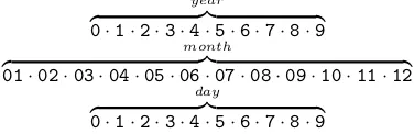
follow-ingtemporal tokens

year

z }| {

0·1·2·3·4·5·6·7·8·9

month

z }| {

01·02·03·04·05·06·07·08·09·10·11·12

day

z }| {

0·1·2·3·4·5·6·7·8·9

Hence, temporal tokens have a vocabulary size of 32. Moreover, for each triple we can extract a sequence ofpredicate tokensthat always consists of the relation type token and, if available, a tem-poral modifier token such as “since” or “until.” We refer to the concatenation of the predicate token sequence and (if available) the sequence of tem-poral tokens as the predicate sequencep_seq. Now, a temporal KG can be represented as a collection of triples of the form (s,p_seq,o), wherein the pred-icate sequence may include temporal information. Table1 lists some examples of such facts from a temporal KG and their corresponding predicate se-quence. We use the suffixy,m anddto indicate whether the digit corresponds to year, month or day information. It is these sequences of tokens that are used as input to a recurrent neural network.

3.1 LSTMs for Time-Encoding Sequences

Fact Predicate Sequence (Barack Obama, country, US) [country]

(Barack Obama, born, US, 1961) [born, 1y, 9y, 6y, 1y]

(Barack Obama, president, US, since, 2009-01) [president, since, 2y, 0y, 0y, 9y, 01m]

Table 1: Facts and their corresponding predicate sequence.

LSTM are

i=σg(hn−1Ui+xnWi)

f =σg(hn−1Uf +xnWf) o=σg(hn−1Uo+xnWo)

g =σc(hn−1Ug+xnWg)

cn=f◦cn−1+i◦g hn=o◦σh(cn)

(3)

wherei,f,oandgare the input, forget, output and input modulation gates, respectively. candhare the cell and hidden state, respectively. All vectors are in Rh. xn ∈ Rd is the representation of the

n-th element of a sequence. In this paper we set

h=d.σg,σcandσh are activation functions.

Each token of the input sequence p_seq is first mapped to its corresponding d-dimensional em-bedding via a linear layer and the resulting se-quence of embeddings used as input to the LSTM. Each predicate sequence of length N is repre-sented by the last hidden state of the LSTM, that is, epseq =hN . The predicate sequence repre-sentation, which carries time information, can now be used in conjunction withsubjectandobject em-beddings in standard scoring functions. For in-stance, temporal-aware versions of TRANSE and

DISTMULT, which we refer to as TA-TRANSE and TA-DISTMULT, have the following scoring

function for triples (s,p_seq,o):

TA-TRANSE:f(s, pseq, o) =||es+epseq−eo||2

TA-DISTMULT:f(s, pseq, o) = (es◦eo)eTpseq.

All parameters of the scoring functions are learned jointly with the parameters of the LSTMs using stochastic gradient descent.

The advantages of character level models to en-code time information for link prediction are: (1) the usage of digits and modifiers such as “since” as atomic tokens facilitates the transfer of informa-tion across similar timestamps, leading to higher efficiency (e.g. small vocabulary size); (2) at test time, one can obtain a representation for a times-tamp even though it is not part of the training set;

(3) the model can use triples with and without tem-poral information as training data. Figure1 illus-trates the generic working of our approach.

4 Experiments

We conducted experiments on four different KG completion data sets where a subset of the facts are augmented with time information.

4.1 Datasets

Integrated Crisis Early Warning System (ICEWS) is a repository that contains political events with a specific timestamp. These political events relate entities (e.g. countries, presidents...) to a num-ber of other entities via logical predicates (e.g. ’Make a visit’ or ’Express intent to meet or ne-gotiate’). Additional information can be found at

http://www.icews.com/. The repository is

organized in dumps that contain the events that occurred each year from 1995 to 2015. We cre-ated two temporal KGs out of this repository, i) a short-range version that contains all events in 2014, and ii) a long-range version that contains all events occurring between 2005-2015. We re-fer to these two data sets as ICEWS 2014 and ICEWS 2005-15, respectively. Due to the large number of entities we selected a subset of the most frequently occurring entities in the graph and all facts where both the subject and object

are part of this subset of entities. We split the facts into training, validation and test in a pro-portion of 80%/10%/10%, respectively. The pro-tocol for the creation of these data sets is identi-cal to the onw followed in previous work ( Bor-des et al.,2013). To create YAGO15K, we used FREEBASE15K(Bordes et al.,2013) (FB15K) as

a blueprint. We aligned entities from FB15K to YAGO (Hoffart et al., 2013) withSAMEAS rela-tions contained in a YAGO dump2, and kept all facts involving those entities. Finally, we aug-ment this collection of facts with time information from the “yagoDateFacts”3dump. Contrary to the

2

/yago-naga/yago3.1/yagoDBpediaInstances.ttl.7z

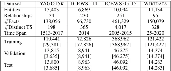
Data set YAGO15K ICEWS ’14 ICEWS 05-15 WIKIDATA

Entities 15,403 6,869 10,094 11,134

Relationships 34 230 251 95

#Facts 138,056 96,730 461,329 150,079

#Distinct TS 198 365 4,017 328

Time Span 1513-2017 2014 2005-2015 25-2020

Training 110,441 72,826 368,962 121,422 [29,381] [72,826] [368,962] [121,422]

Validation 13,815 8,941 46,275 14,374

[3,635] [8,941] [46,275] [14,374]

Test 13,800 8,963 46,092 14,283

[3,685] [8,963] [46,092] [14,283]

Table 2: Statistics of the data sets. TS stands for timestamps. The number of facts with time information is in brackets.

YAGO15K WIKIDATA

MRR MR Hits@10 Hits@1 MRR MR Hits@10 Hits@1

TTRANSE 32.1 578 51.0 23.0 48.8 80 80.6 33.9

TRANSE 29.6 614 46.8 22.8 31.6 50 65.9 18.1

DISTMULT 27.5 578 43.8 21.5 31.6 77 66.1 18.1

TA-TRANSE 32.1 564 51.2 23.1 48.4 79 80.7 32.9 TA-DISTMULT 29.1 551 47.6 21.6 70.0 198 78.5 65.2

Table 3: Results (filtered setting) of the temporal knowledge graph completion experiments for the data sets YAGO15Kand WIKIDATA. The best results are written bold.

ICEWS 2014 ICEWS 2005-15

MRR MR Hits@10 Hits@1 MRR MR Hits@10 Hits@1

TTRANSE 25.5 148 60.1 7.4 27.1 181 61.6 8.4

TRANSE 28.0 122 63.7 9.4 29.4 84 66.3 9.0

DISTMULT 43.9 189 67.2 32.3 45.6 90 69.1 33.7

TA-TRANSE 27.5 128 62.5 9.5 29.9 79 66.8 9.6 TA-DISTMULT 47.7 276 68.6 36.3 47.4 98 72.8 34.6

Table 4: Results (filtered setting) of the temporal knowledge graph completion experiments for the data sets ICEWS 2014 and ICEWS 2005-15. The best results are written bold.

ICEWS data sets, YAGO15Kdoes contain tempo-ral modifiers; namely, ’occursSince’ and ’occur-sUntil’. Contrary to previous work (Leblay and Chekol,2018), all facts maintain time information in the same level of granularity as one can find in the original dumps these data sets come from.

We also experimented with the temporal facts from the WIKIDATAdata set4extracted in (Leblay and Chekol, 2018). Only information regarding the year is available for these facts, since the authors discarded information of finer granular-ity. All facts are framed in a time interval (i.e. they contain the temporal modifiers ’occursSince’ and ’occursUntil’). Facts annotated with a single point-in-time are associated with that time-point as start and end time. Due to the large number of entities of this data set, which hinders the com-putation of standard KG completion metrics, we selected a subset of the most frequent entities and

4_{http://staff.aist.go.jp/julien.leblay/datasets}

kept all facts where both thesubjectandobjectare part of this subset of entities. This set of filtered facts was split into training, validation and test in the same proportion as before.

Table 2 lists some statistics of the temporal KGs. All four data sets, with their corresponding training, validation, and test splits are available at

https://github.com/nle-ml/mmkb.

4.2 General Set-up

We evaluate various methods by their ability to answer completion queries where i) all the argu-ments of a fact are known except thesubjectentity, and ii) all the arguments of a fact are known except

the object entity. For the former we replace the

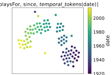
[playsFor, since, temporal_tokens(date)]

1920

1940

1960

1980

2000

date

Figure 2: T-SNE visualization of the embed-dings learned for the predicate sequence p_seq = [playsFor, occursSince, date], where date corre-sponds to the date token sequence.

This is standard procedure in the KG completion literature. We also report the filtered setting as de-scribed in (Bordes et al.,2013). The mean of all computed ranks is the Mean Rank (lower is bet-ter) and the fraction of correct entities ranked in the top nis called hits@n(higher is better). We also compute the Mean Reciprocal Rank (higher is better) which is less susceptible to outliers.

Recent work (Leblay and Chekol,2018) evalu-ates different approaches for performing link pre-diction in temporal KGs. The approach that learns independent representations for each timestamp and use these representations as translation vec-tors, similarly to (Bordes et al., 2013), leads to the best results. This approach is called VECTOR

-BASED TTRANSE, though for the shake of sim-plicity in the paper we refer to it as TTRANSE. We compare our approaches TA-TRANSE and

TA-DISTMULT against TTRANSE, and the standard embedding methods TRANSE and DISTMULT. For all approaches, we used ADAM (Kingma and Ba, 2014) for parameter learning in a mini-batch setting with a learning rate of 0.001, the cate-gorical cross-entropy (Kadlec et al.,2017) as loss function and the number of epochs was set to 500. We validated every 20 epochs and stopped learn-ing whenever the MRR values on the validation set decreased. The batch size was set to 512 and the number of negative samples to 500 for all ex-periments. The embedding size is d=100. We ap-ply dropout (Srivastava et al.,2014) for all embed-dings. We validated the dropout from the values

{0,0.4}for all experiments. For TA-TRANSE and

TA-DISTMULT, the activation gateσg is the

sig-moid function;σcandσhwere chosen to be linear

activation functions.

20 50

Epoch

1.5

Training Loss

TransE

TA-TransE

Figure 3: Training loss in YAGO15K. TA-TRANSE’s ability to learn from time information leads to a lower loss.

4.3 Results

Table3 and4 list the results for the KG comple-tion tasks. TA-TRANSE and TA-DISTMULT sys-tematically improve TRANSE and DISTMULT in MRR, hits@10 and hits@1 in almost all cases. Mean rank is a metric that is very susceptible to outliers and hence these improvements are not consistent. TTRANSE learns independent

repre-sentations for each timestamp contained in the training set. At test time, timestamps unseen dur-ing traindur-ing are represented by null vectors. This explains that TTRANSE is only competitive in YAGO15K, wherein the number of distinct times-tamps is very small (see#Distinct TS in Table2) and thus enough training examples exist to learn robust timestamp embeddings. TTRANSE’s per-formance is similar to that of TA-TRANSE, our time-aware version of TRANSE, in WIKIDATA. Similarly, TTRANSE can learn robust timestamp representations because of the small number of distinct timestamps of this data set.

Figure3shows a comparison of the training loss of TRANSE and TA-TRANSE for YAGO15K. Under the same set-up, TA-TRANSE’s ability to learn from time information leads to a training loss lower than that of TRANSE.

Figure 2 shows a t-SNE (Maaten and Hinton,

2008) visualization of the embeddings learned for the predicate sequencep_seq = [playsFor, occursS-ince,date], wheredatecorresponds to the date to-ken sequence. This illustrates that the learned rela-tion type embeddings carry temporal informarela-tion.

5 Conclusions

References

J. van Benthem. 1995. Handbook of logic in artificial intelligence and logic programming (vol. 4). chapter Temporal Logic, pages 241–350. Oxford University Press, Inc., New York, NY, USA.

Antoine Bordes, Nicolas Usunier, Alberto Garcia-Duran, Jason Weston, and Oksana Yakhnenko. 2013. Translating embeddings for modeling multi-relational data. In Advances in neural information processing systems, pages 2787–2795.

Melisachew Wudage Chekol, Giuseppe Pirr`o, Jo-erg Schoenfisch, and Heiner Stuckenschmidt. 2017. Marrying uncertainty and time in knowledge graphs. InAAAI, pages 88–94.

Melisachew Wudage Chekol and Heiner Stucken-schmidt. 2018. Rule Based Temporal Inference. In

Technical Communications of the 33rd International Conference on Logic Programming (ICLP 2017), volume 58, pages 4:1–4:14, Dagstuhl, Germany. Schloss Dagstuhl–Leibniz-Zentrum fuer Informatik.

Maximilian Dylla, Iris Miliaraki, and Martin Theobald. 2013. A temporal-probabilistic database model for information extraction. Proc. VLDB Endow., 6(14):1810–1821.

C. Esteban, V. Tresp, Y. Yang, S. Baier, and D. Krompa. 2016. Predicting the co-evolution of event and knowledge graphs. In2016 19th International Con-ference on Information Fusion (FUSION), pages 98–105.

Alberto Garcia-Duran and Mathias Niepert. 2017. Kblrn: End-to-end learning of knowledge base rep-resentations with latent, relational, and numerical features. arXiv preprint arXiv:1709.04676.

Kelvin Guu, John Miller, and Percy Liang. 2015. Traversing knowledge graphs in vector space. arXiv preprint arXiv:1506.01094.

Johannes Hoffart, Fabian M Suchanek, Klaus Berberich, and Gerhard Weikum. 2013. Yago2: A spatially and temporally enhanced knowledge base from wikipedia. Artificial Intelligence, 194:28–61.

Tingsong Jiang, Tian Yu Liu, Tao Ge, Lei Sha, Baobao Chang, Sujian Li, and Zhifang Sui. 2016. Towards time-aware knowledge graph completion. In COL-ING.

Rudolf Kadlec, Ondrej Bajgar, and Jan Kleindienst. 2017. Knowledge base completion: Baselines strike back. arXiv preprint arXiv:1705.10744.

Yoon Kim, Yacine Jernite, David Sontag, and Alexan-der M Rush. 2016. Character-aware neural language models. InAAAI, pages 2741–2749.

Diederik P Kingma and Jimmy Ba. 2014. Adam: A method for stochastic optimization. arXiv preprint arXiv:1412.6980.

Julien Leblay and Melisachew Wudage Chekol. 2018. Deriving validity time in knowledge graph. In

Companion Proceedings of the The Web Conference 2018, WWW ’18. International World Wide Web Conferences Steering Committee.

Laurens van der Maaten and Geoffrey Hinton. 2008. Visualizing data using t-sne. Journal of machine learning research, 9(Nov):2579–2605.

Maximilian Nickel, Kevin Murphy, Volker Tresp, and Evgeniy Gabrilovich. 2016. A review of relational machine learning for knowledge graphs. Proceed-ings of the IEEE, 104(1):11–33.

Nitish Srivastava, Geoffrey Hinton, Alex Krizhevsky, Ilya Sutskever, and Ruslan Salakhutdinov. 2014. Dropout: A simple way to prevent neural networks from overfitting. The Journal of Machine Learning Research, 15(1):1929–1958.

Rakshit Trivedi, Hanjun Dai, Yichen Wang, and Le Song. 2017. Know-evolve: Deep temporal rea-soning for dynamic knowledge graphs. In Pro-ceedings of the 34th International Conference on Machine Learning, volume 70 of Proceedings of Machine Learning Research, pages 3462–3471, In-ternational Convention Centre, Sydney, Australia. PMLR.

Bishan Yang, Wen-tau Yih, Xiaodong He, Jianfeng Gao, and Li Deng. 2014. Learning multi-relational semantics using neural-embedding models. arXiv preprint arXiv:1411.4072.