Similarity and Pattern Recognition
Chun-Hung Tzeng, Computer Science Department
Ball State University, Muncie, IN 47306, U.S.A., [email protected]
Abstract—This paper formally defines similarities as tolerance relations, which are reflexive and sym-metric binary relations. An abstract set with a simi-larity is called a tolerance space. The training data set in a learning task is a given database of independent identically distributed random pairs (Xi, Yi), where eachXi is a record andYi is its label: Yi∈ {0,1}. The goal of the learning is to design a classifier of which the error probability is near to the theoretical limita-tion, the Bayes error. The learning process consists of finding a similarity of feature vectors ψ(Xi)’s and the learning result is a representative data clustering on the tolerance space of feature vectors. The infor-mation about a record X derived from the represen-tative clustering is the set of represenrepresen-tatives similar to the feature vector ψ(X). The percentage of the records of class 1 in the intersection of these repre-sentative clusters is used to estimate the conditional probability of Y = 1. This paper defines aθ-classifier, which assigns the record to class 1 if the conditional probability is larger than the thresholdθ. If the clus-tering is a partition, the threshold θ = 1
2 minimizes error probability in the training data set. In general, an optimal θ-classifier has a different threshold. The experiments show the trade-off between the number of clusters and the error probabilities of the optimal
θ-classifiers.
Keywords: similarity, tolerance-space, representative-clustering, pattern-recognition, classification
1
Introduction
Pattern recognition is about guessing or predicting the unknown nature of an observation, a discrete quantity such as black or white, abnormal or normal, one or zero, sick or healthy, real or fake. Usually, an observation is a collection of numerical measurements such as an im-age or a vector of weather data ([3, 9]). Formally, an observation is a d-dimensional vector x. The unknown nature is aclass, which is denoted by yand takes values in a finite set C ={0,1,2, ..., M}. The task is to create a function g : Rd −→ C. The value g(x) represents the
guess ofy, givenx. The functiong is called aclassifier. The classifier errs on x if g(x) 6= y. In a probabilistic setting (e.g., [3]), we consider a random pair (X, Y) on
Rd× C, of which a distribution describes the frequency
of encountering particular pairs in practice. The proba-bility of error for a classifiergisL(g) =P(g(X)6=Y). A best possible classifier g∗ which has the minimal
proba-bility of error is calledBayes classifierorBayes rule. The minimal probability of error is called theBayes error.
In the two-class problemC ={0,1}, the Bayes classifier is defined byg∗(x) = 1 iff η(x)>1/2, where η(x) is the
posterior probability η(x) =P(Y = 1|X =x). In most cases, the distribution of (X, Y) and the Bayes classifier
g∗ are unknown. To design a classifier is based on a
given database of pairs (Xi, Yj),1≤i≤n. Such a task
is called a supervised learning. Many classification rules have been proposed (e.g., [3, 9]). For example, the k -nearest neighbor rulegn(x) takes a majority vote over the
Yi’s in subset ofkpairs (Xi, Yi) from the given database
that have the smallest valueskXi−xk.
Similarities or dissimilarities play a central role in the pattern recognition, implicitly or explicitly. For example, the k-nearest neighbor rule uses the Euclidean distance to measure similarities. Most similarity measures are re-flexive and symmetric. That is, eachxis not dissimilar to itself and the similarity measure of twox’s is independent of the order ofx.
This paper introduces a probabilistic model for the two-class pattern recognition on an abstract space Ω based on a formally defined similarity, called a tolerance rela-tionand denoted byξ. The similarityξis a reflexive and symmetric binary relation on Ω. The pair Ωξ = (Ω, ξ)
is called atolerance space. Zeeman [19] introduced toler-ance relation to describe the imperfection of human sight. A representative system of a tolerance space was studied in [17]. More references on tolerance relation are in [13].
In the tolerance space, the neighborhood of an elementx
isξ(x) ={u∈Ω :ξ(x, u)}, the set of all elements similar to x. Let Fξ be the Borel field generated by all such
neighborhoods. The probabilistic model is constructed on the measurable space (Ωξ,F
ξ). The pattern recognition
problem is represented by a random pair (X, Y),X ∈Ω and Y ∈ {0,1}. A classifier is a measurable function
g : Ω −→ {0,1}, which errs on X if g(X) 6=Y. Bayes rule is extended to this model, which is based on the posterior probabilityη(x) =P(Y = 1|X ∈x), wherexis the minimal measurable set containingx. Bayes error is also defined.
This paper designs classifiers based on a training data set, a database of pairs (Xi, Yi), where 1≤i≤n, the record
the sequence (X1, Y1), ...,(Xn, Yn) is a sequence of
inde-pendent identically distributed (i.i.d.) random pairs. Let Ωn ={Xi|1≤i≤n}. A data pre-processing is formally
represented by a function ψ : Ωn −→ Φ. The image of
the function Φm=ψ(Ωn) is the feature vector set of the
training data set. The cardinality |Φm| is usually much
smaller than|Ωn|for computational purpose.
For each feature vector x ∈ Φm, we store the
frequen-cies of Y in the training data set in n0(x) and n1(x), which are the numbers of records of class 0 and class 1 in ψ−1(x)⊆Ω
n, respectively. On the training data set,
the conditional probability Y = 1, given ψ(X) = x, is
ηΦm(x) =
n1(x)
n0(x)+n1(x). The Bayes error based on this
con-ditional probability should near the original Bayes error. Otherwise, the data pre-processing should be redesigned.
On Φm, we define a similarity ξ and consider the
toler-ance space (Φm)ξ, on which we apply the data
cluster-ing introduced in [16] and find a representative system
Rξ ={R1, R2, ..., Rk}of the space.
Each feature vector in Φm is similar to at least one Ri.
For eachi, the cluster represented byRi is its
neighbor-hood ξ(Ri). Such a data clustering is not a partition
in general. Two clusters may have non-empty intersec-tion. Rξ is minimal if there is no smaller representative
system. Maak [12] introduced the concept of minimal representative system to approximate the mean value of some functions on abstract groups. In this paper, we use a minimal representative system to represent a pattern learned from the training data set.
Consider a random pair (X, Y). Given the value ofX, we derive information aboutX from the representative sys-temRξ. We find the representatives similar to the feature
vector ψ(X), denoted by NX ={R1′, ..., R′k′}, and
con-sider their intersection, denoted byFX. Lett0 andt1 be
the record numbers of class 0 and class 1 in the subset
ψ−1(F
X) of the training data set, respectively. On the
training data set, the conditional probability of Y = 1, given ψ(X)∈FX, is η(X) = t0+t0t1. We use this
condi-tional probability to estimate the posterior probability of any recordX.
The θ-classifier (θ ∈ [0,1]) is defined by gθ(X) = 1 iff
η(X)> θ. If the clusteringRξ is a partition, thenθ=12
minimizes the error probability (e.g., [15]). In general, we need to find an optimal thresholdθ0for the minimal error probability. The error probability ofgθ0 on the training
data set is a performance indicator. The similarityξneed to be adjusted if the error probability does not near the Bayes error based on conditional probabilityηΦm. This
paper does not consider other criteria, such as false pos-itive. The experiments in the paper show that the error probability of theθ0-classifier for the testing data set can be well predicted for proper similarities.
The remainder of this paper is organized as follows: tion 2 reviews tolerance space and data clustering. Sec-tion 3 introduces the probabilistic model of pattern recog-nition. Section 4 introduces the supervised learning and
θ-classifiers. Section 5 describes the experiments. Section 6 is the conclusion.
2
Tolerance Space and Representative
Clustering
In this section, we define a similarity formally. Let Ω be an abstract set of elements.
Definition 2.1 A tolerance relation ξ on Ω is a binary
relation with two conditions: (x, x) ∈ ξ for any x ∈ Ω (reflexivity), and (x, y)∈ξ⇒(y, x)∈ξ(symmetry). The pair (Ω, ξ) is called a tolerance space, denoted by Ωξ. We also use ξ as a predicate: ξ(x, y) iff (x, y) ∈ ξ.
If ξ(x, y), we say that x is ξ-similar to y, or x and
y are ξ-similar. We omit ξ when there is no ambigu-ity. On a metric space (M, d), for example, each posi-tive real number ε > 0 defines a tolerance relation dε:
dε(x, y) ifd(x, y) < ε, x, y ∈ M. Any undirected graph
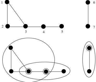
can be treated as a tolerance space (and vice versa), where Ω is the set of all vertices, and two vertices are similar if they are the same vertex or they are adjacent (e.g., Figure 1). Any equivalent relationξ on Ω is a tol-erance relation having the transitive property.
The set inclusion⊆is a partial ordering on tolerance rela-tions on Ω. The collection of all tolerance relarela-tions forms a lattice with a unique lower bound and a unique upper bound. The lower bound is called the discrete tolerance relation, which is{(x, x) | x ∈ Ω} (i.e., each element x
is similar only to itself). We call the corresponding tol-erance space thediscrete tolerance space, denoted by Ω0.
The upper bound is called the trivial tolerance relation, which is Ω×Ω (i.e., any two elements are similar). The corresponding tolerance space is called the trivial toler-ance space, denoted by Ω∞.
4
6
7 3
1
2
[image:2.595.334.518.574.731.2]5
For eachx∈Ω, the setξ(x) ={u∈Ω :ξ(x, u)}, consist-ing of all elements similar tox, is called theneighborhood
of x. Let Fξ be the Borel field generated by all
neigh-borhoods. The pair (Ωξ,F
ξ) is a measurable space and
each element of Fξ is called a ξ-measurableset. For
ex-ample, consider Ω = Rn, the n-dimensional Euclidean
space, and the tolerance relationξ(x, y) iff kx−yk < ε
for a fixed given ε > 0, where kx−yk is the Euclidean distance. Then the correspondingFξ is the collection of
all Borel sets inRn.
For any x ∈ Ωξ, the singleton {x} is not always ξ
-measurable (i.e., in Fξ). In Figure 1, for example, {1},
{2}, {6}, and {7} are not ξ-measurable, and the single-tons {3}, {4}, and {5} are ξ-measurable. We define in-distinguishable elements as follows.
Definition 2.2. Two elementsxanduin Ωξ are
indis-tinguishable, denoted by x ∼ u, if they have the same neighborhood (i.e.,ξ(x) =ξ(u)).
Note that ∼is an equivalent relation. Let x={u|u∼
x}, the set of all indistinguishable elements of x, which is called the indistinguishable set of x and satisfies x =
T
u∈ξ(x)ξ(u)−
S
u6∈ξ(x)ξ(u). In Figure 1, for example,
1 = 2 = {1,2} and 6 = 7 ={6,7}. To avoid advanced measure theory (e.g., [10]), we assumexisξ-measurable for anyx∈Ω and is the smallest ξ-measurable set con-tainingx. This assumption is always true if Ω is a count-able set.
A function from a tolerance space to another tolerance space f : Ωξ −→Φζ is calledmeasurableiff−1(A)∈ F
ξ
for all A ∈ Fζ. A measurable function maps
indistin-guishable sets into indistinindistin-guishable sets.
Theorem 2.3. If x ∼ y in Ωξ and the function f :
Ωξ −→Φζ is measurable, thenf(x)∼f(y) in Φζ.
Proof. Let a = f(x). Since a is ζ-measurable and x
is the smallest ξ-measurable set containing x, the in-versef−1(a) isξ-measurable and containsx. Therefore, f(y)∈aandf(x)∼f(y).
For any real-valued measurable functionf on Ωξ,f(x) =
f(u) ifx∼u(considering the Borel sets of real numbers). Especially, every real-valued measurable function on the trivial tolerance space Ω∞ is a constant function.
Any function from a set to a tolerance space defines a tolerance relation on the domain. Suppose thatf : Ω−→
Φζ is a function from an arbitrary set Ω to a tolerance
space Φζ. We define a tolerance relationξ
ζ on Ω:ξζ(x, u)
for x, u∈Ω if f(x) and f(u) are ζ-similar in Φζ. Then
the function f : Ωξζ −→Φζ is measurable. For example,
in a data pre-processingf : Ω−→Φ, f(x) is the feature vector ofx. Each similarity on the feature vectors defines a similarity on the original data set Ω.
We review the data clustering in a tolerance space Ωξ
[16]. Here we assume that Ωξ is finite. Each x ∈ Ω is
called a representative of its neighborhood ξ(x). A set of elements {r1, ..., rk} is called a representative system
of the tolerance space Ωξ if the corresponding
neighbor-hoods cover the whole space Ω. A representative system
{r1, ..., rk} isminimal if there is no other representative
system with less thankmembers. In this paper, we call such a minimal representative system aminimal represen-tative clustering. Note that the clustering in this paper is not crisp in general and two clusters may have non-empty intersection. Such a property is important in the uncertainty study of AI [18] and is different from many clustering algorithms (e.g., [8]).
To search for a minimal representative clustering is in-tractable in general. We introduce a heuristic search [16] which uses a concept of density. The density func-tion on Ω is the number of elements in ξ(x): den(x) =
|ξ(x)|. According to den(x), we sort the elements of Ω: x1, x2, ..., xm, so that den(x1) ≥ den(x2) ≥ ... ≥
den(xm). To search for a representative system, choose
the neighborhoodξ(x1) first. Then choose the next neigh-borhoodξ(xi) (according to the density order) which is
not covered by previously chosen neighborhoods. Repeat the process until the whole space is covered. Finally, scan the chosen neighborhoods backwards and delete the neighborhood which is contained in the union of other al-ready collected neighborhoods. In this paper, we use such a sub-minimal representative system to approximate a minimal representative clustering. Figure 1 shows a min-imal representative clustering computed by the heuristic method.
3
Bayes Classifier and Bayes Error
Pattern recognition is about guessing or predicting the unknown nature of an observation, a discrete quantity such as black or white, one or zero, sick or healthy, ab-normal or ab-normal. An observation is a collection of in-formation about an object, such as an image, a vector of weather data, or an internet message. Note that about the object the information of an observation is not al-ways complete and has some degree of uncertainty. The observation usually is represented by a vector of several components and each component may be numerical or categorical. Formally, we usexto denote an observation and Ω to denote the space of all possible observations. The unknown nature of the observation is called aclass. It is denoted by y and takes values in a finite set. For simplicity, this paper considers only two possible classes (e.g., normal and anomaly), denoted by 0 and 1. In pat-tern recognition, one creates a function g : Ω −→ {0,1}
which represents one’s guess of y given x. The map-pingg is called aclassifier. The classifier errs onxwhen
Definition 3.1 A probability measure on a tolerance space Ωξ is a probability measure µ on the measurable
space (Ωξ,F
ξ). The triple (Ωξ,Fξ, µ) is a called a
prob-ability space of Ωξ.
Given a probability space (Ωξ,F
ξ, µ), each measurable
functionf : Ωξ −→Φζ defines a probability measureµ ζ
on (Φζ,F
ζ) as follows. For any measurable set A∈ Fζ,
µζ(A) = µ(f−1(A)). The triple (Φζ,Fζ, µζ) is a
proba-bility space. For example, the function f is a feature se-lection and any probability measure on the original data is transformed to the feature vectors.
Letξbe a tolerance relation on Ω and (Ωξ,F
ξ, µ) a
prob-ability space. If there is no ambiguity, we omit the ξ in our notation. Let (X, Y) be a random pair taking their respective values from Ω and {0,1}. The random pair may be defined by a pair (µ, η), where µis the probabil-ity measure ofX andηis the regression ofY onX. That is, for anyA∈ F,P(X ∈A) =µ(A),and for anyx∈Ω,
η(x) = P(Y = 1|X ∈x). Note thatη is measurable and
η(x) =η(y) ifxandy are indistinguishable.
A classifier is a measurable function g : Ω −→ {0,1}. Here we treat {0,1} as a discrete tolerance space. The probability of error L(g) = P(g(X) 6= Y) is called the
errorofg, which is the integration of a conditional prob-ability:
L(g) =P(g(X)6=Y) =
Z
Ω
P(g(X)6=Y|X ∈x)dµ(x)
Definition 3.2TheBayes classifieris defined as follows
g∗(x) =
1 ifη(x)>1/2,
0 otherwise.
The errorL(g∗) is called theBayes Error. Similarly to
the classical Bayes rule [3], we can prove
Theorem 3.3The Bayes classifier minimizes the error;
that is, for any classifierg,L(g∗)≤L(g).
The Bayes error L(g∗) is the theoretical limitation of
the performance of any designed classifier g. Note that
L(g∗) = 0 if η(x) ∈ {0,1} for all x ∈ Ω. The goal of this paper is to construct a classifier to approximate the Bayes error as near as possible.
4
Optimal
θ
-Classifier
Training Data Set
The Bayes classifierg∗dependsupon the tolerance space Ωξ and the distribution of
(X, Y). In most cases, both the tolerance relation ξand the distribution are not given so that both Bayes classi-fier and Bayes error are unknown. To design a classiclassi-fier is usually based on a given database of pairs (Xi, Yi),
1≤i≤n. The database may be the result of experimen-tal observations. It could also be obtained through an ex-pert or teacher who filled in theYi’s after having seen the
Xi’s. To find a classifier with a small error is hopeless
un-less there is some assurance that the (Xi, Yi)’s jointly are
some representatives of the unknown distribution. Here, we assume the data (i.e., (X1, Y1), ...,(Xn, Yn)) is a
se-quence of independent identically distributed (i.i.d.) ran-dom pairs with the same distribution as that of (X, Y). To construct a classifier on the basis ofX1, Y1, ..., Xn, Yn
is calledlearning, supervised learning, orlearning with a teacher. The given database is called the training data set. In this section, we introduce a process of construct-ing such a classifier usconstruct-ing similarities on the trainconstruct-ing data set.
EachXiin the training data set usually consists of several
components, each of which may be numerical or categori-cal. We also assume that the class ofXiis binary; that is,
Yi∈ {0,1}. Let Ωn be the set of allXi’s: Ωn ={Xi|1≤
i ≤ n}. Note that |Ωn| ≤ n because it is possible that
Xi=Xj for differenti andj. For eacht∈Ωn, consider
two counts: f0(t) = |{i | 1 ≤ i ≤ n, Xi = t, Yi = 0}|
and f1(t) =|{i | 1≤i ≤n, Xi =t, Yi = 1}|. Note that P
t∈Ωn(f0(t) +f1(t)) =n. Then on the training data set
(as a discrete space), the conditional probability ofY = 1, given X =t, is ηn(t) =
f1(t)
f0(t)+f1(t). Let the
correspond-ing Bayes classifier and Bayes error (on Ωn) be denoted
byg∗
n andLn(gn∗), respectively. Note that Ln(gn∗) = 0 if
Xi 6= Xj for any i =6 j. The Bayes error Ln(g∗n) is the
theoretical limitation of the learning. If the Bayes error is too large, the performance of the learning result will be poor. Usually, larger data set or more information for eachX is needed.
Data Pre-processing
Before designing a classifi-cation scheme, a data pre-processing is commonly ap-plied to the training data set, such as data cleaning, data integration, data granulation, feature extraction, data transformation, and data reduction (e..g, [8, 9]). Formally, we use a function to represent the data pre-processing, ψ : Ωn −→ Φ. For convenience, we calleach sample X a record and ψ(X) thefeature vector of
X. All possible feature vectors form the set Φ. Usu-ally the function ψis not one-to-one. For the frequency of Yi, we store two integers for each feature vector x:
n0(x) = |{i | 1 ≤ i ≤ n, ψ(Xi) = x, Yi = 0}| and
n1(x) = |{i | 1 ≤ i ≤ n, ψ(Xi) = x, Yi = 1}|. That is,
n0(x) and n1(x) are the numbers of records of class 0 and class 1 inψ−1(x)⊆Ω
n, respectively. Let the image
of Ωn be denoted by Φm =ψ(Ωn) (⊂ Φ). Usually, the
size of Φmis much smaller than that of Ωnfor the
compu-tational purpose. Note thatP
x∈Φm(n0(x) +n1(x)) =n.
Consider Φm as a discrete space. For each x∈Φm, the
conditional probability of Y = 1 on the training data set, given ψ(X) = x, is ηΦm(x) =
n1(x)
n0(x)+n1(x). Let the
corresponding Bayes classifier and Bayes error (on Ωn)
be denoted byg∗
Φm and Ln(g
∗
Φm), respectively. The
fea-ture vector ψ(X) may not contain all information of X
pre-processing simplifies the computation, still the Bayes errorLn(gΦ∗m) should be near toLn(g
∗
n). If the difference
between the two errors is too large, the pre-processingψ
should be re-designed.
Representative Classification Scheme
On Φ we define a suitable tolerance relation (i.e., similarity), denoted by ξ. To define similarity depends on each in-dividual task and there are many methods to measure similarities or dissimilarities (e.g., [9]). Here we simply assumeξ is given. Consider representative clustering on the tolerance space (Φm)ξ and letRξ ={R1, R2, ..., Rk}be a sub-minimal representative system computed by the algorithm introduced in Section 2.
Deciding whether an event is surprising is one of the tasks in statistics [6, 7]. Here we also define a concept of surprising records with respective to the tolerance space (Φm)ξ. The tolerance relationξis first transformed to the
training data set. Two recordsXiandXj in the training
data set are similar if the corresponding feature vectors
ψ(Xi) andψ(Xi) are similar. A record t∈ Ωn is called
a surprise if t is not similar to any other record in Ωn
and there is only one ifor which Xi =t. Letx=ψ(t).
Then t is a surprise iff ψ−1(x) ={t}, the neighborhood ξ(x) = {x} is a singleton in the tolerance space (Φm)ξ,
and n0(x) +n1(x) = 1. Therefore, the feature vector of a surprise is always inRξ.
Let the numbers of the surprises of class 0 and class 1 be denoted by αξ and βξ, respectively, which are
in-dependent of the choice of Rξ. Finally, we use L =
(Φm, Rξ, αξ, βξ) to represent the result computed
above, which is called a representative classification scheme.
θ
-Classifiers
Consider the random pair (X, Y). Given the value ofX, we design classifiers ofX based on a rep-resentative classification scheme L = (Φm, Rξ, αξ, βξ)as follows. We find the representatives (inRξ) similar to
the feature vectorψ(X), denoted byNX ={R1′, ..., R′k′}.
First consider the case that NX is not empty. Let the
intersection of the clusters of these representatives be
FX = Tk
′
i=1ξ(R′i), which is the set of all feature
vec-tors (in Φm) similar to all representatives in NX. If
FX =∅, then it is replaced by the union of the clusters:
FX =
Sk′
i=1ξ(R′i). The set FX is a piece of information
aboutX derived fromL, from which we compute poste-rior probability ofY.
In the subset ψ−1(F
X) of Ωn, the number of records of
class 0 is t0 =P
x∈FXn0(x) and the number of records
of class 1 ist1=P
x∈FXn1(x).On the training data set,
the conditional probability ofY = 1, givenψ(X)∈FX, is t1
t0+t1. For any random sample (X, Y), we use this value
to predict the conditional probability, which is denoted by ηL(X) = P(Y = 1| L) = t0+t1t1. Next if NX = ∅,
that is,ψ(X) is not similar to any of the representatives
in Rξ, then we say that the record X is an unknown
surprise(w.r.t. L). Ifαξ+βξ >0, then the conditional
probability is estimated as ηL(X) = P(Y = 1| L) = βξ
αξ+βξ. If αξ+βξ = 0, then we say that the conditional
probability of unknown surprises is not predictable, that is, ηL(X) is undefined. Note that all unknown surprises
have the same predicted conditional probability and will be classified to one class; therefore, the similarity should be modified if there are too many surprises in the training data set.
In the following we introduce a simple non-randomized classifier using a threshold, without considering any loss function. Let θ, 0< θ < 1, be a real number, then we define the following classifier:
Definition 4.1Theθ-classifieris defined as follows
gθ(X) =
1 ifηL(X)> θ,
0 ifηL(X)≤θ,
unknown ifηL(X) is undefined.
The error ofgθon the training data set can by computed,
denoted by LL(θ) = Ln(gθ), which satisfies Ln(g∗n) ≤
Ln(g∗Φm) ≤ LL(θ). The error LL(θ) is an indicator of
the performance of the classifiergθ. If the representative
clusteringRξis a partition of Φm, the errorLL(θ) reaches
its minimum at θ = 12. In the special case that ξ is the discrete tolerance relation (i.e., each element in Φm
is a representative in Rξ), this error is the Bayes error:
Ln(g∗Φm) =LL( 1
2). In the other extreme case that ξ is
the trivial tolerance relation (i.e., there is only one cluster inRξ), the information derived fromLis the numbers of
records of class 1 and class 0 in the training data set. Therefore, the classifier will classifies all records to class 1 or 0, depending on the fact that the record number of class 1 in the training data set is larger or not. In general,
Rξ is not a partition andg1
2 does not have the minimal
error.
Definition 4.2 Thegθ0 is called an optimal θ-classifier
if
LL(θ0)≤LL(θ), 0< θ <1.
Since Φm is finite, an optimal θ-classifier can be
com-puted. If the error LL(θ0) (on the training data set) is
too far away from the Bayes errorLn(g∗Φm), new
similar-ities should be considered. This paper considers only the probability of error and does not consider other criteria, such as false positive. The experiments in the next sec-tion show that the error of theθ-classifier on testing data set can be well predicted for proper similarities.
5
Experiments
la-beled with normal or certain attack. The 42nd attribute is the label, of which there are 23 different types: one is normal and others are attacks. All attacks are classified as anomalies in the experiments. We use 0 to represent a normal and 1 to represent an anomaly. Our task is to classify records based on the 41 attributes into two classes: anomaly or normal.
Pre-Processing and Training Data Set
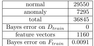
Not all 41 features are significant in the classification task. The traditional statistical test of the equality of two dis-tributions is used in this process. We select an attribute to the feature vector if the distributions of the value domains are significantly different for the two types of records. We have selected 9 attributes. Each categorical value is labeled by an integer. The values of continuous attributes are granulated into a linearly ordered discrete values according to their distribution. Each record t is mapped into a feature vectorψ(t). By a few feature vec-tors, 85.08% (139213 records in total) of total records are classified perfectly. Those records are not used in the experiments in order to make the error more visible.From the rest of the records, we choose randomly about half of normals and half of anomalies as the training data set, and the rest as the testing data set. Let the train-ing data set be denoted by Dtrain and the testing data
set by Dtest. The Dtest consists of 29603 normals and
7310 anomalies, 36913 in total. Letψ(Dtrain) be denoted
by Ftrain. The numbers of records inDtrain andFtrain
and the corresponding Bayes errors are shown in Table 1. Note that the pre-processing reduces the number of the records from 36845 to 1160 (3.1% of 36845). It also reduces the number of features from 41 to 9. The Bayes error is raised from 0 to 0.0091.
normal 29550
anomaly 7295
total 36845
Bayes error onDtrain 0
[image:6.595.305.508.278.416.2]feature vectors 1160 Bayes error onFtrain 0.0091
Table 1: Information about the training data set.
Tolerance Relations and
θ
-classifiers
On fea-tures vectors we define a generalized Hamming distance, denote byd. For eachε >0, we define a tolerance relation on feature vectors: dε(f, g) if d(f, g)≤ε.Consider the training process on the tolerance space (Ftrain)dε. For a representative classification schemeLε
= (Ftrain, Rdε, αdε, βdε), we study the θ-classifier gθ.
In this paper, we introduce some results for differentε’s: 0.01, 0.5, 2.0, and 9.0. For ε = 0.01, (Ftrain)d0.01 is the
discrete space, in which all 1160 feature vectors are rep-resentatives and the clustering is a partition. Therefore, the Bayes classifier (on Dtrain) is an optimalθ-classifier
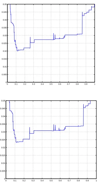
(i.e., θ0 = 0.5). For other two cases, the clusterings are not partitions. The cluster numbers and computations are significantly reduced, but errors increase. The exper-iment result is summarized in Table 2, which shows the trade off between the computations and errors. Further-more, the error functionsLLε(gθ) are depicted in Figure
2 forε= 0.5. The top one is forDtrain and the bottom
one is for Dtest.
If ε is sufficiently large (e.g. ε ≥ 9.0), then all records are indistinguishable. That is, the only information used in this case aboutDtrain is that there are 29550 normals
and 7295 anomalies and ηL(X) = 0.1959 for any X.
Therefore, each record will be classified as a normal. The error of this classifier is 0.1980, but no anomalies are classified at all.
ε |Rdε| α β θ0 train-error
0.01 1160 236 92 0.50 0.0091 0.5 240 12 17 0.11 0.0202 2.0 38 0 0 0.60 0.1012 9.0 1 0 0 0.50 0.1980
ε unknown surprises test-error
0.01 339 0.0132
0.5 121 0.0236
2.0 19 0.1048
[image:6.595.93.245.495.570.2]9.0 0 0.1980
Table 2: Information about some classification
models and optimal θ-classifiers.
6
Conclusion
This paper introduces a probabilistic classification model on a tolerance space. Similarities are formally defined as reflexive and symmetric binary relations. Probability measures are constructed on the measure space generated by neighborhoods in the space. Training data set is a database of pairs (Xi, Yi), where eachXi is a record and
Yi is the label (0 or 1) of the record. The data
pre-processing maps the records in the training data set to feature vectors.
The learning process includes search for similarities of feature vectors. For each similarity, the learning result is a representative clustering of the tolerance space of feature vectors. The information about a given record is the set of representatives similar to the feature vector of the record. In the intersection of the corresponding clusters, the percentage of records of class 1 is used to predict the posterior probability of the given record. The
0 0.1 0.2 0.3 0.4 0.5 0.6 0.7 0.8 0.9 1 0
0.005 0.01 0.015 0.02 0.025 0.03 0.035 0.04 0.045 0.05
0 0.1 0.2 0.3 0.4 0.5 0.6 0.7 0.8 0.9 1 0
[image:7.595.87.251.77.388.2]0.005 0.01 0.015 0.02 0.025 0.03 0.035 0.04 0.045 0.05
Figure 2: Error ofθ-classifiers forε= 0.5.
to class 1 if the posterior probability is larger thanθ. An optimal threshold is not necessarily 12 in general.
A concept of surprising record is introduced. The model assigns the same posterior probability to all unknown surprises. Therefore, the learning process should avoid similarities with too many surprises. The experiments demonstrate the trade-off between computations and classification errors.
Future works include more experiments and more investi-gation on the mathematical theory of the model, such as the handling of surprises and other criteria of classifiers.
References
[1] Berger, J. O., Statistical Decision Theory and Baysian Analysis, 2nd Edition, Springer-Verlag, 1985.
[2] Brun, M., Sima, C., Hua, J., Lowey, J., Carroll, E. S., Shu, E., Dougherty, E. R., “Model-based eval-uation of clustering validation measures,” Pattern Recognition40, pp. 807-824, 2007.
[3] Devroye, L, and Gy¨orffi, G. Lugosi, A Probabilistic Theory of Pattern Recognition, Springer, 1996.
[4] Dougherty, E. R., and Brun, M., “A probabilistic theory of clustering,” Pattern Recognition 37, pp. 917-925, 2004.
[5] Dunham, M. H.,Data Mining, Introductory and Ad-vanced Topics, Prentice Hall, 2003.
[6] Good, I. J.,THE ESTIMATION OF PROBABILI-TIES, An Essay on Modern Bayesian Methods, Re-search Monograph No.30, MIT Press, Cambridge, Mass., 1965.
[7] Good, I. J.,The Foundations of Probability and Its Applications University of Minnesota Press, Min-neapolis, 1983.
[8] Han, J. and Kamber, M.,Data Mining Concepts and Techniques, 2nd Edition, Morgan Kaufmann, 2006.
[9] Hastie, T, Tibshirami, R. and Friedman, J.,The El-ements of Statistical Learning, Springer, 2001.
[10] Jacobs, K., Measure and Integral, Academic Press, 1978.
[11] KDD-99 Cup Dataset
http://kdd.ics.uci.edu/databases/kddcup99.html
[12] Maak, W., Fastperiodische Funktionen, Springer-Verlag, 1967.
[13] Schroeder, M. J. and Wright, M. H., “Tolerance and Weak Tolerance Relations,”Journal of Combinato-rial Mathematics and CombinatoCombinato-rial Computing11, pp. 123-160, 1992.
[14] Sun, F.-S. and Tzeng C.-H., “Classification and Anomaly Detection in Tolerance Space,”Proc. of the Ninth IASTED International Conference on Intelli-gent Systems and Control, pp. 206 - 211, Honolulu, Hawaii, 2006.
[15] Tzeng, C.-H. A Theory of Heuristic Information in Game-Tree SearchSpringer-Verlag, 1988.
[16] Tzeng, C.-H. and Sun, F.-S., “Data Clustering in Tolerance Space,” in Berthold, Lenz, Bradley, Kruse, and Borgelt, editors, Advances in Intelligent Data Analysis V, Springer-Verlag pp. 297-306, 2003.
[17] Tzeng, C.-H. and Tzeng, C.-S. O., “Tolerance spaces and almost periodic functions,” Bull. Inst. Math. Acad. Sinica6, pp.159-173, 1978.
[18] Zadeh, L., “A New Direction in AI Toward a Compu-tational Theory of Perceptions,”AI MagazineSpring 2001, pp. 73-84.