A Model for Potential Deterministic Effects in Turbomachinery Flows

A Model for Potential Deterministic Effects in

Turbomachinery Flows

Stefan Stollenwerk

and Dirk Nuernberger

Abstract—The unsteady interaction between blade rows due to a potential field is very important in highly loaded compressors because of its impact on operating performance. In this context the interac-tions of a flat plate wake with an upstream running pressure wave is investigated numerically using the compressible Navier-Stokes solver TRACE. Several flow conditions regarding Reynolds number, pressure wave amplitude and the axial position of the wave en-try plane are examined.

The observed phenomena and dependencies are used to develop a transport model which adds determin-istic stresses by means of source terms to the sta-tionary simulation. Calculations based on the pro-posed model are described and compared with the time-accurate and steady-state numerical simulations. The model captures the influence of the unsteady ef-fects on the time-mean flow accurately and yields a speedup factor of approximately two orders of mag-nitude compared to time-accurate simulations.

Keywords: Aerodynamics, Turbomachinery, Blade Row Interaction, Deterministic Stresses, Numerical Methods

Nomenclature

κ Streamline curvature

μd Deterministic pseudo-viscosity

μl Molecular viscosity

ρ Density

τij Viscous shear stress tensor

d Axial distance

kd Deterministic kinetic energy

p Pressure

t Time

ui Velocity

xi Coordinate direction

S Source term for transport equation

Superscripts

ˆ

φ Stochastic perturbation ˆ

ˆ

φ Deterministic perturbation

φ Density-weighted stochastic perturbation

∗_{stefan.stollenwerk@dlr.de} †_{dirk.nuernberger@dlr.de}

Institute of Propulsion Technology, German Aerospace Center (DLR), 51147 Cologne, Germany

φ Density-weighted deterministic perturbation

φ Ensemble-average

φ Density-weighted ensemble-average

φ Time-passage average

φ Density-weighted time-passage average

1

Introduction

An improved understanding of unsteady flow phenomena is especially important in turbomachinery aerodynamics where significant unsteadiness occurs. One topic in this field is blade row interaction in highly loaded configura-tions, especially in transonic compressors where moving shock waves interact with the upstream blade row wakes. The experimental investigation using PIV and static pres-sure meapres-surements performed by Sanders and Fleeter [9] showed that the trailing edge stagnation point moves pe-riodically from the pressure to the suction surface of the upstream blade row due to this shock interaction. The resulting vorticity and loss generation was quantified by Gorrell et al. [6]. Langford et al. [8] noticed a direct relationship between different shock strengths and their influence on the size and intensity of the shed vortices. At subsonic operating conditions, remarkable potential effects also exist even if they appear much weaker com-pared to transonic regimes. However, the downstream potential flow field influences the wakes of the upstream blade row as it disturbs and therefore deflects the up-stream wake structures in the circumferential direction of the rotor movement.

Due to the trend towards small axial spacing in modern compressor technology many researchers focused on the influence of blade row spacing on loss producing and per-formance. They found that the efficiency decreases with increasing axial spacing in transonic flow regimes, while under subsonic operating conditions, the efficiency rises with increasing axial spacing, cf. Zachcial and Nuern-berger [13].

inexpen-sive tools using the standard stationary mixing-plane ap-proach do not include the unsteady effects linked with the rotational speed of the rotor. The flow variables on either side of the mixing-plane are circumferentially aver-aged which implies a loss of information associated with an unphysical entropy jump at the interface.

The proposed transport model couples physical accuracy with computational efficiency. After the presentation of the applied numerical methods and the test vehicle, the results of unsteady parameter studies are shown and dis-cussed. The parameters chosen are the shock strength, the Reynolds number and the axial position of the shock entry plane which represents the axial row distance in real compressors.

The developed model is described. The mathematical derivation is followed by an identification of the corre-lations drawn from the time-accurate parameter studies. The model is then applied and the achieved results are compared to time-accurate and stationary mixing-plane data to point out its utility.

2

Numerical Method and Test Case

Both the time-accurate and the steady-state simulations are carried out with the parallel 3D multi block solver TRACE. The code has been developed at DLR’s Institute of Propulsion Technology and is optimised for turboma-chinery flows. The Navier-Stokes equations are solved using Roe’s TVD upwind scheme to discretize the con-vective fluxes and central differences for the derivatives of the viscous fluxes on structured or unstructured multi-block grids. The implicit time-integration scheme allows large CFL numbers and a fast convergence rate. Tur-bulence modelling is effected by ak-ω two-equation ap-proach with turbomachinery-specific extensions. Several additional modules extend the solver’s applicability to aeroelastic, aeroacoustic, multi-phase and real gas prob-lems.

The considered test case in the current numerical study is a flat plate in a subsonic flow regime with a Mach number of M a= 0.6. A pressure wave propagates upstream to simulate highly loaded compressor configurations. The pressure disturbance is prescribed mathematically at the exit. Peak and shape of the pressure wave in the di-rection along the exit planes are derived from real high pressure compressors of today’s civil aero engines. Fig. 1 shows the computational domain with three different exit planes (A, B and C). In this study they are employed to analyze the effect of distance on the interaction of the pressure disturbance with the trailing edge. The distance between the trailing edge and the exit plane of gridA is

d, grid B elongates this distance about 50% and grid C

duplicates it. The two-dimensional structured grids are refined in the boundary layer and wake region. Mesh A

comprehends 28778, mesh B 30056 and mesh C 31192 grid points.

Figure 1: Computational grid with labeled exit planes (every second gridline is shown)

3

Unsteady Parameter Studies

A turbocompressor operates under various working con-ditions. Some important parameters that define a par-ticular state are investigated regarding their influence on the flowfield. These are the Reynolds number, the pres-sure wave amplitude and the axial distance of blade rows represented by different exit planes or wave entry planes respectively. The angle of inclination and the speed of the upstream propagating wave front were also varied but the corresponding results did not show an interdependence, so they are not considered in this paper. The achieved results served as a data basis for the model development. In order to characterize and identify the unsteadiness, we define a deterministic kinetic energy:

kd=

1 2

ˆ ˆ

u12+ ˆu2ˆ2+ ˆu3ˆ2

(1)

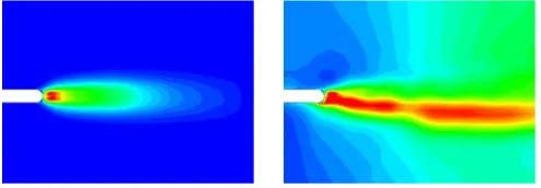
Note that the velocity fluctuations in this expression are related to the rotor frequency. The turbulent analogy to this expression is known as turbulent kinetic energy and contains the stochastic perturbations. In the left picture of Fig. 2, a contour plot of the deterministic kinetic en-ergy without any shock involvement is shown. A small

Figure 2: Deterministic kinetic energy without and with shock interaction

upper side, the wake is further offset to the lower side. The corresponding picture of the flowfield with interact-ing shock yields the right part of Fig. 2.

Re1552817 Re2746856 Re31105630

p∗₁= 0.75 - A

-p∗2= 1.00 A A, B, C A

p∗₃= 1.25 - A

-Table 1: Parameter Combinations

Table 1 indicates the grid on which a given parameter combination is calculated (Fig. 1). p∗i is the related peak

value of the pressure wave generated at the particular exit. p∗1 therefore lies 25% under this level, whilep∗3

ex-ceedsp∗2 about the same value. Rei shows the Reynolds

number that determines the flow field. Additional values of all of the given parameters were examined, but are not presented in this paper since they do not provide any fur-ther information.

Considering different amplitudes of the pressure wave, it is not surprising that the influence on the wake profile rises with the pressure peak strength, which is clearly shown in the right picture of Fig. 3 where one dimen-sional velocity profiles at the exit of the domain A are shown. Since the disturbance amplitude cannot be ex-pressed by a steady simulation, there is only one steady profile in comparison to the three different unsteady re-sults. The time-averaged wakes are widened and offset compared to the steady wake as can be seen by the asym-metry of the averaged unsteady velocity profile. The steady velocity deficit is about 20 % higher than in the time-averaged case. At the trailing edge (left picture of Fig. 3), the difference in axial velocity is even smaller. The averaged unsteady deficit is about 50 % lower than the steady one, but there is no noticeable widening. Ap-parently, the wave amplitude has no influence on the av-eraged unsteady velocity shape because all profiles lie on top of each other. It is very likely that the considered pressure waves are of an insufficient strength since they do not evoke additional vortices.

Figure 3: Pressure peak variation - velocity profiles at the trailing edge and at the exit of gridA

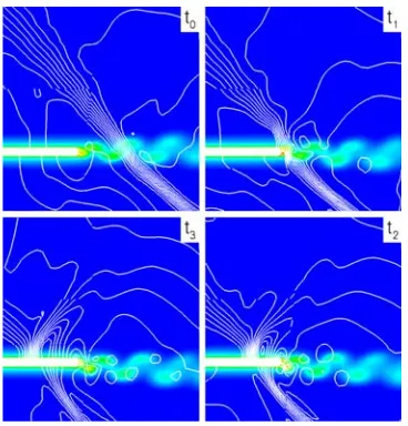
To underline this statement, Fig. 4 shows the motion of a pressure wave front withp∗3that impinges on the trailing

Figure 4: Time-varying entropy field with isobars at four different time steps

edge of the plate. The entropy contours remain nearly unchanged apart from a slight wake bending due to the direction of wave propagation as mentioned above. In case of a Reynolds number variation, there is also no difference in the wake profiles at the trailing edge. Here, the Von K´arm´an vortex street is dominant too and there-fore hardly influenced by the Reynolds number. At the exit plane of gridA, a widening of the wake goes along with a reduced velocity deficit compared to the steady results. The influence on the flowfield decreases with an increasing Reynolds number when the inertial forces grow relating to the viscous forces in the fluid. The left picture in Fig. 5 illustrates this behaviour. In the right picture the influence of the axial spacing is shown. The larger the axial distance between the trailing edge and the pres-sure wave entry plane the smaller is the influence on the wake. There is a considerable upstream decay of the wave intensity.

4

Model

4.1

Model development

This section describes how the deterministic stresses can be included in a stationary solver. Explicit details on the average-passage equation system can be found in Adam-czyk [1]. Here the derivation of the reduced form of this approach is presented, cf. Hall [7]. The equation system is developed through the consecutive application of two averaging operations applied to the Navier-Stokes equa-tions. The procedure is described for the momentum equation; the continuity equation and the energy equa-tion can be derived in a similar way. The momentum equation reads as follows:

∂

∂t(ρui) + ∂ ∂xj

(ρuiuj) =−∂p

∂xi

+ ∂

∂xjτij

(2)

First, the instantaneous field is subjected to a Reynolds decomposition, i.e. a decomposition into a mean part and a turbulent fluctuation:

φ=φ+ ˆφ (3)

The ensemble-averageφis defined as:

φ= lim

N→∞ 1 N N n=1

φn (4)

Introducing the density-weighted ensemble-averaging (Favre-averaging):

φ=ρφ

ρ ⇒φ

_{=φ−φ (5)}

The mass weighted splitting is applied to the velocity field, the flow variableρandpare decomposed according to (3). An ensemble-average procedure on the momentum equation leads to:

∂(ρui)

∂t +

∂(ρuiuj)

∂xj

=−∂p

∂xi

+ ∂

∂xj

⎡ ⎢

⎣τij− ρu iuj Reynolds stress

⎤ ⎥ ⎦ (6)

This is well-known as theRANS-formulation. The addi-tional term that has arisen through this process is referred to as the Reynolds stresses and is typically represented through the use of turbulence models.

To illustrate the deterministic portion in the equation, the mean quantityφ is further decomposed into a time-passage averaged part and an unsteady deterministic fluc-tuation:

φ=φ+φˆˆ (7)

The averaging procedure consists of a time averaging over the time period ΔT depending on the dominating fre-quency of the unsteadiness, and a summation averaging [10]:

φ= 1

N N n=1 1 ΔT

_t0+ΔT

t0

¯

φn(t)dt (8)

The density-weighted time-passage averaging now reads:

φ=ρφ

ρ ⇒φ

_{=φ−φ (9)}

Introducing (7) into (6) and applying (8) and (9) one obtains the equation system that underlies the presented deterministic model:

∂

∂t(ρui) + ∂ ∂xj

(ρuiuj)

=−∂p

∂xi

+ ∂

∂xj

⎡ ⎢

⎣τij−ρuiuj − ρu iuj Det. stress

⎤ ⎥ ⎦ (10)

The key issue in this study is the modelling of the addi-tional deterministic stress termρu_iu_j. According to the unsteady results, the deterministic stresses can be corre-lated with the local velocity gradient. Therefore Boussi-nesq’s approximation can be applied without a pressure term:

ρuiuj =μd

∂ui

∂xj

+∂uj

∂xi

(11)

In other approaches using deterministic stresses, each of the six deterministic stress components has to be mod-eled separately. Additionally, as can be seen in [2] or [12], these methods normally employ one transport equa-tion per stress component. In contrast, the presented approach is easier to implement and provides more com-putational efficiency. The transport mechanism ofμd is

described with:

ρ∂μd

∂t + (ρui) ∂μd

∂xi −

(μl+μd)∂

2_μ

d

∂x2_i =S (12)

The main effort underlying this study consists of model-ing the source termS consisting of two different terms:

S =S1+S2 (13)

The first term represents the origin of the deterministic stress production in those regions with high velocity fluc-tuations. These regions correlate with the local stream-line curvature. The termS1is therefore a function of the streamline curvature and the Reynolds number:

The bending of the streamlines is very strong immedi-ately behind the trailing edge. This reflects the physical mechanism of vortex formation and the consequent stress production at this location. The stresses are transported in the downstream direction which is represented by the convection term in the transport equation.

In the time-accurate reference-simulations, it was ob-served that the mixing process in the downstream convec-tion leads to a rise in deterministic stresses because the amplitude of the responsible propagating pressure wave decays in the upstream direction. This effect is modeled by the second source term which has the form of an ex-ponential function:

S2=f(μd, p∗, d, x) (15)

S2 depends mainly on the strength of the potential per-turbation and on the axial distance between the blade rows. As it is a decay function, the axial coordinate x

also takes part of the formulation. The parameter stud-ies mentioned above were used to develop and to calibrate this term.

4.2

Results

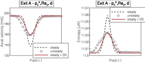
Applying the deterministic stress model in the stationary solver, the one dimensional velocity profiles of the wake are strongly improved towards the averaged unsteady re-sults. The left picture of Fig. 6 compares the three calcu-lated velocity profiles at the exit of gridA. The considered pressure amplitude accounts top∗₂, the Reynolds number isRe2and the axial distance isd. The right picture shows the corresponding entropy distribution under the same flow conditions. The model predicts a better loss distri-bution compared to the stationary solution. As the

ver-Figure 6: Velocity (left) and entropy (right) profiles of an unsteady, steady and DS-model calculation

tical direction of the wave front motion is not considered in the model, the asymmetry of the wake profiles could not be reproduced. Beside this fact, the DS-model shows an excellent agreement with the referenced averaged un-steady results. In Fig. 7 the velocity profiles are shown for two other wave strengths calculated. It shows that the wake asymmetry increases with the pressure ampli-tude. Fig. 8 shows the velocity profiles at the exit plane of gridAfor two different Reynolds numbers. Regarding

Figure 7: Wake profiles of an unsteady, steady and DS-model calculation for two different pressure amplitudes

Figure 8: Wake profiles of an unsteady, steady and DS-model calculation for two different Reynolds numbers

the remaining parameterdthat represents the axial dis-tance between the two blade rows, Fig. 9 also shows that the model yields good results even if the considered wake profiles are not yet strongly widened.

Figure 9: Wake profiles of an unsteady, steady and DS-model calculation for two different axial distances

5

Conclusions and Future Work

configura-tions. In the first instance, this should be done on a two dimensional basis before considering fully three dimen-sional simulations. The far goal is to include the deter-ministic stress model in the aerodynamic design process in the turbomachinery industry.

References

[1] Adamczyk J.J., “Model Equation for Simulating Flows in Multistage Turbomachinery”, ASME Pa-per No. 85-GT-226, 1985

[2] Charbonnier, D., Leboeuf, F., “Steady Flow Simula-tion Of Rotor Stator InteracSimula-tions With A New Un-steady Flow Model”, AIAA Paper No. 2004-3754, 2004

[3] Eulitz, F., Nuernberger, D., and Schmitt, S., “Numerical Modelling of Unsteady Turbomachinery Flow”,Proceedings 5th European Congress on Com-putational Methods in Applied Sciences and Engi-neering, Barcelona, Spain, 2000

[4] Gorrell, S.E., Okiishi, T.H., and Copenhaver, W.W., “Stator-Rotor Interactions in a Transonic Compres-sor: Part I - Effect of Blade-Row Spacing on Perfor-mance”,Proceedings of ASME Turbo Expo 2002, Pa-per No. GT-2002-30494, Amsterdam, The Nether-lands, 2002

[5] Gorrell, S.E., Okiishi, T.H., and Copenhaver, W.W., “Stator-Rotor Interactions in a Transonic Compres-sor: Part II - Description of a loss Producing Mecha-nism”, Proceedings of ASME Turbo Expo 2002, Pa-per No. GT-2002-30495, Amsterdam, The Nether-lands, 2002

[6] Gorrell, S.E., Car, D., Puterbaugh, S.L., Estevade-ordal, J., and Okiishi, T.H., “An Investigation of Wake-Shock Interactions in a Transonic Compressor With Digital Particle Image Velocimetry and Time-Accurate Computational Fluid Dynamics”, Trans-actions of the ASME, 128, pp. 616-626, 2006

[7] Hall, E.J., “Aerodynamic Modeling of Multistage Compressor Flowfields - Part 2: Modeling Determin-istic Stresses”, ASME Paper No. 97-GT-345, 1997

[8] Langford, M.D., Breeze-Stringfellow, A., Guillot, S.A., Solomon, W., Ng, W.F., and Estevadeordal, J., “Experimental Investigation of the Effects of Blade-Row Spacing on the Flow Capacity of a Transonic Compressor Stage”,ASME Journal of Turbomachin-ery, 17, pp. 43-48, 2005

[9] Sanders, A.J., Fleeter, S., “Transonic Rotor-IGV In-teractions”,ISABE Paper No. 99-7029, 1999

[10] Stridh, M., Modeling of Unsteady Flow Effects in Throughflow Calculations, ISRN CTH-TFD-PB-03/07, Goeteborg, Sweden, 2003

[11] Turner, M.G., Gorrell, S.E., and Car, D., “Radial Migration of Shed Vortices in a Transonic Rotor Fol-lowing a Wake Generator: A Comparison Between Time Accurate and Average Passage Approaches”,

ASME Paper No. GT-2005-68776, 2005

[12] van de Wall, A.G., Kadambi, J.K., Adamczyk, J.J., “A Transport Model for the Deterministic Stresses Associated With Turbomachinery Blade Row Inter-actions”, ASME Journal of Turbomachinery, 122, pp. 593-603, 2000