Determining a regular language by glider based structures called phases fi 1 in Rule 110

Reprints available directly from the publisher Published by license under the OCP Science imprint, Photocopying permitted by license only a member of the Old City Publishing Group

Determining a Regular Language by

Glider-Based Structures called Phases f

_i

₋

1

in Rule 110

Genaro J. Martínez1,∗, Harold V. McIntosh2, Juan C. Seck Tuoh Mora3and Sergio V. Chapa Vergara4

1_{Faculty of Computing, Engineering and Mathematical Sciences,}

University of the West of England, Bristol, United Kingdom E-mail: [email protected]

2_{Departamento de Aplicación de Microcomputadoras,}

Instituto de Ciencias, Universidad Autónoma de Puebla, Puebla, México E-mail: [email protected]

3_{Centro de Investigación Avanzada en Ingeniería Industrial,}

Universidad Autónoma del Estado de Hidalgo Pachuca, Hidalgo, México E-mail: [email protected]

4_{Departamento de Computación,}

Centro de Investigación y de Estudios Avanzados del Instituto Politécnico Nacional, México E-mail: [email protected]

Received: November 1, 2006. Accepted: February 1, 2007.

Rule 110 is a complex elementary cellular automaton able of support universal computation and complicated collision-based reactions between gliders. We propose a representation for coding initial conditions by means of a finite subset of regular expressions. The sequences are extracted both from de Bruijn diagrams and tiles specifying a set of phases fi−1 for each glider in Rule 110. The subset of regular expressions is explained in detail.

Keywords: Cellular automata, Rule 110, de Bruijn diagrams and regular

expres-sions.

1 INTRODUCTION

The study of the binary-state one-dimensional cellular automaton Rule 110 has had a certain attention before and after the demonstration that its evolution space can bear universal computable processes (see [5, 34]).

Another important and complementary result to the previous one was obtained by Turlough Neary and Damien Woods showing that the problem

of predictingtsteps in Rule 110 is P-complete. Some interesting reductions of

Turing machines are displayed in [28]. On the other hand, Kenichi Morita has finished a complicate and new results in cyclic tag systems [11, 12]. Mainly over the “halt” condition in this system.

The diversity of problems in Rule 110 and its possible applications in differ-ent fields determine the necessity of formalizing a represdiffer-entation for coding systematically the evolution rule; for easily constructing initial conditions which define a control of the gliders (particles or mobile localizations) taking part in simple or complicated complex operations.

In the present paper we report a set of sequences based on gliders that can be represented as regular expressions codified in initial conditions offering a way to manipulate the glider system in Rule 110.

The paper gives a brief introduction to Rule 110 and its glider system. Later it presents a small review on regular languages, de Bruijn diagrams and tiles. Finally it explains how the expressions are calculated for all the gliders up to now known in Rule 110 (without extensions), illustrating a simple procedure to handle collisions between gliders and depicting some relevant constructions. A pertinent mention is that this set of regular expressions has been successfully applied in some of our previous results in Rule 110 [13,14,16–18].

2 BASIC NOTATION

Rule 110 is a cellular automaton of order(k=2, r=1)(Wolfram’s notation)

evolving in one dimension, wherek determines the number of states of an

alphabetandris the number of cells considered both to the left and to the

right side with regard of a central cell.

Particularly, Rule 110 can produce a wide variety of gliders on a periodic background called “ether” by Matthew Cook [4, 5]. Thus, Rule 110 belongs to Class IV in Wolfram’s classification.

The local function determining the behavior of Rule 110 is:

ϕ(0,0,0)→0 ϕ(1,0,0)→0

ϕ(0,0,1)→1 ϕ(1,0,1)→1

ϕ(0,1,0)→1 ϕ(1,1,0)→1

ϕ(0,1,1)→1 ϕ(1,1,1)→0

TABLE 1 Evolution rule 110

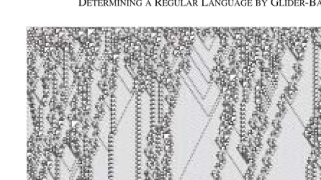
FIGURE 1

Random evolution in Rule 110.

starting from linear array of cells each containing one state of; taking every

cellxi as a central one, we evaluate the value of its corresponding

neighbor-hood to determine the new central element in the following generation:

ϕ(x_it₋₁, xt_i, x_it₊₁)→xt_i+1.

Timetis discrete and there is a simultaneous evaluation of eachxi in the

array, i.e., parallel mappings generate the following array, determining the

evolution spaceZ.

Figure 1 shows a typical random evolution in Rule 110 with an initial density of 0.5 in an array with 723 cells for 363 steps. In the evolution we have applied a filter identifying the ether configurations allowing a clear recognizing of the gliders present in this example.

Once established the existence of gliders (particles or mobile localizations) we must classify them and determine their properties.

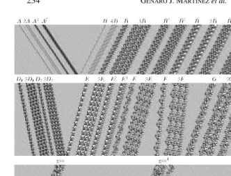
3 GLIDER SYSTEM IN RULE 110

In this section we show all the gliders until now known in Rule 110. Let us use the classification proposed by Cook [5] from now on (illustrated in Figure 2). Gliders are presented in two forms: as a simple structure and as extensions or packages of them (one example showed in Figure 2). Each glider with superscriptn∈Z+represents that it can arbitrarily extend; extensions to the

left are defined inB¯ andBˆ gliders, and extensions to the right are withE

andGgliders. At the end of the list there is an extended glider gun, where the

extension is originated byE¯ gliders. Also, we can see examples of extended

gliders and packages with their respective notation.

FIGURE 2

Glider classification in Rule 110.

from right to left is realized byB,B¯,Bˆ,E,E¯,F,G,Hgliders and the glider gun. The last trajectory is with gliders which does not have a shift,C1,C2and

C3gliders. Each glider has a period determined by the number of generations

among shifts letting the same sequence or the change fromxi toxi+dorxi−d,

whered ∈Zrepresents the number of places crossed in every period.

An important indication is that the set of regular expressionsR110

describ-ing all the gliders in Rule 110 does not include extensions or packages of them, it is only for simple gliders. On trying to enumerate all those extensions or packages, the set of expressions grows in different modules; therefore, the

number of sequenceswin the set is the union of the periods for every glider:

R110= p

i=1

wi,g∀(wi ∈∗∧g∈G) (1)

whereGis the whole set of gliders in Rule 110 andp≥3 is the corresponding

period. This way, we can speak of a regular languageLR110that is constructed

from the expressions ofR110. We must notice that this language is a subset

of the whole language in Rule 110, that is, it is only the one defined by the expressions representing gliders, then we have:

LanguageLR110is based on the regular expressionsR110 determining

each glider; a remarkable comment is thatLR110has not been published or

explained by other authors.

LR110is established by the de Bruijn diagrams and the characterization of

the tiles, where both have been analyzed for defining useful features called “phases.” The phases indicate with precision both the position and the exact moment where each glider must be positioned into a given initial condition.

When applying the set of regular expressions and their basic operations we are able to construct desired initial conditions which yield evolutions with important characteristics; the main interest is to control and produce collisions among gliders. In this wayLR110is a powerful tool to codify initial conditions

in Rule 110, and this subset has been implemented in a computer system. Immediate applications with relevant results in the study of Rule 110 has been performed over hundreds, thousands, millions and thousands of million of cells, as we shall see in the following section.

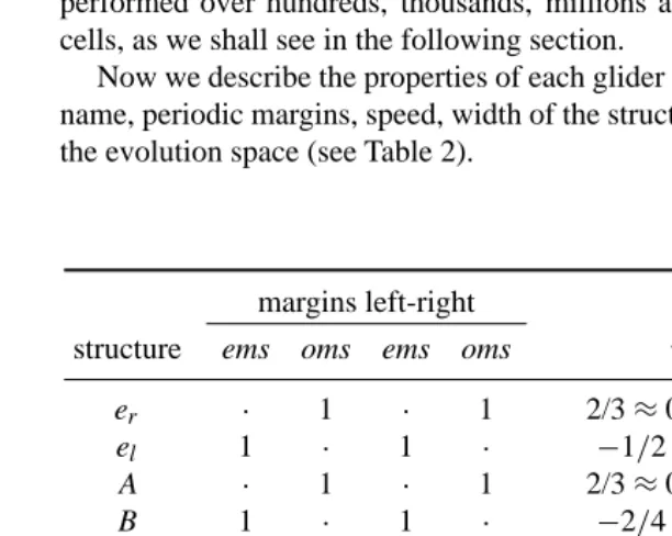
Now we describe the properties of each glider in different aspects such as: name, periodic margins, speed, width of the structure and the cap by glider in the evolution space (see Table 2).

margins left-right

structure ems oms ems oms vg width cap

er · 1 · 1 2/3≈0.666666 14 T

el 1 · 1 · −1/2= −0.5 14 T

A · 1 · 1 2/3≈0.666666 6 T

B 1 · 1 · −2/4= −0.5 8 P

¯

Bn 3 · 3 · −6/12= −0.5 22 T

ˆ

Bn 3 · 3 · −6/12= −0.5 39 T

C1 1 1 1 1 0/7=0 9–23 P

C2 1 1 1 1 0/7=0 17 P

C3 1 1 1 1 0/7=0 11 P

D1 1 2 1 2 2/10=0.2 11–25 P

D2 1 2 1 2 2/10=0.2 19 P

En 3 1 3 1 −4/15≈ −0.266666 19 P

¯

E 6 2 6 2 −8/30≈ −0.266666 21 P

F 6 4 6 4 −4/36≈ −0.111111 15–29 P

Gn 9 2 9 2 −14/42≈ −0.333333 24–38 P

H 17 8 17 8 −18/92≈ −0.195652 39–53 P

glider gun 15 5 15 5 −20/77≈ −0.259740 27–55 P

TABLE 2

In Table 2, column structure represents the name of the glider or periodic structure. The following four columns labeled margins, indicate the number of periodic margins in each glider. The margins are divided in margins with even values ‘ems‘ and odd values ‘oms’ which are distributed as well in two groups: left and right, because gliders has even and odd margins in their left or right borders (or superior and inferior ones). Particularly, the properties of the mar-gins are explained in subsection 4.4, discussing their orimar-gins, interpretations and representations.

Columnvg∀g∈Gindicates the speed of each glider, where it is calculated

dividing the shiftd between its periodp. The three types of trajectories are

identified in this column. Positive speed indicates a shift to the right, negative speed a shift to the left and a zero speed tells that the glider does not have a shift.

Column width indicates the minimum and maximum number of necessary cells for determining a periodic chain in the linear array forming a glider or

another periodic structure. For example, for theC1glider we have two values,

this means that with nine or twenty-three cells may define this glider in the initial condition.

The last column cap indicates the gliders able to completely cover the evolution space of Rule 110. The cap can be total ‘T’ or partial ‘P,’ where total cap implies a glider which does not need additional tiles to completely cover the evolution space. A partial cap describes that at least the intervention of another tile is necessary so that the glider and the new tile can completely cover the evolution space. This representation is oriented to the problem established by McIntosh to cover the space with different tiles and to find the combination of gliders fulfilling this condition.

Thus, another tendency in the research is represented by looking for pos-sible complex constructions through tiles rather than using initial conditions.

From an initial set of tilesXwe can construct a family of different setsXi

so that, {X ⊂ · · · ⊂ Xi ⊂ Xi+1 ⊂ · · · }and each set must produce a

dif-ferent pattern, hence we will make operations with the tiles in the cartesian plane as in a puzzle but without violating the valid connections determined by Rule 110. Therefore, in the sense of Hao Wang, we can find a composition of different setsXito implement a sequence of tiles being operated by a

logi-cal function, describing another way of universal computation based on these constructions [7].

4 DETERMINING A GLIDER-BASED REGULAR LANGUAGE IN RULE 110

the finite subset of glider-based regular expressions. Both approaches give ori-gin to the interpretation of “phases” in Rule 110; once determined the phases, a procedure is explained to control specific collisions among gliders

codi-fied into initial conditions applying the subsetR110of regular expressions

establishing a regular languageLR110.

4.1 Tiles in Rule 110

A plane of tiles T is a countable family of closed sets T = {T0, T1, . . .}

covering the plane without intervals or intersections [7]. Defined as a join of sets (called a mosaicT):

T =

n

i=0

Ti∀n∈Z+0 (3)

The “plane” is the Euclidian planeZ×Zin elementary geometry.

Rule 110 covers the evolution space through different sets of trianglesTn∀ n∈Z+₀, wherenrepresent the size of the triangle counting the cells in some of its internal sides. The tiles are divided in two sets:αandβ∀n≥2 [22] (each setαorβdetermines its own countable family of tiles where|{T_nα}| = |{Tnβ}|,

as illustrates Figure 3). For example, differentαandβtiles are present in the

construction of both theHglider and the glider gun (see Figure 4 in [16]).

We can represent aT0tile by state 0; with this when the initial

configura-tion is covered by the expressions: 0*, 1* and (10)*, the evoluconfigura-tion space is established by a homogenous evolution with state 0 (or tileT0). Nevertheless,

the behavior is not the same for tilesT1, T2α, T β 2, T3α, T

β

3, . . . , Tnα, T β n, . . . .

The evolution space can be covered by anyTntiles for 0≤n≤4. Thus for

n≥5 the evolution space is covered by at least twoTntiles. LetTiandTj∈T

wherei=j, then both sets cannot operate in the plane under the function of

Rule 110 if they cover the space partially (gaps) or overlap in their cells. Another question is to know the largest tile that Rule 110 can construct

in its evolution space. At the present time, the limit is established by aT45

tile [23]; therefore, Rule 110 cannot construct a greater mosaic. At the moment there is a way to produceTntiles where 0≤n ≤ 33; tilesT43,T44 andT45

were calculated through a specialized search determining the ancestors for each tile [23]. Finally, other open problem is to determine a construction for tiles in the interval 34≤n≤42.

FIGURE 3

Thus, the tile family{T_nα}and{Tnβ}allows a detailed description of the

evolution space in Rule 110 through their sets:αandβ. A second important

point is that the tiles establish properties by the periodic margins in their recurrent structures (gliders and ether). Their interpretation is very important to derive the phases, including non-periodic structures.

As we said before, if from an initial setXa family of different setsXi is

defined so that{X⊂. . .⊂Xi ⊂Xi+1⊂. . .}, a function:T∗→T∗can

be defined. Thus, we have eachn_i=0Ti =Xi ⊂GwhereXi =GN∨GC.1

4.2 Regular expressions

Several interesting problems rise in the study of formal languages; one of them is to determine the type of language derived and to which class belongs. This hierarchy is well-known and established by Chomsky’s classification. We shall study languages determined by regular sets, since the set of expressions determined by each glider in Rule 110 can be associated to a particular regular expression. Thus, some concepts of finite state machines are needed.

The finite automaton is a mathematical model with a system of discrete inputs and outputs; the system can be placed in one of a finite set of states. This state has the information of the received inputs necessary to determine the behavior of the system with regard of subsequent inputs. Formally, a finite

automatonM consists of a finite set of states and a set of transitions among

states induced by the symbols selected from some alphabet. For each symbol there is a transition form one state to other (it can return to the same one); there is an initial state where the automaton stars and some states are designated as final ones or acceptance states [9].

A directed graph called a transition diagram is associated with a finite automaton as follows: the vertices of the graph correspond to the states of the automaton; for a transition from stateito statejproduced by an input symbol,

there is an edge labeled by this symbol fromitoj in the transition diagram.

The finite automaton accepts a chainwif the analogous transition sequence

leads from the initial state to a final one (or acceptation).

A language accepted by M, represented by L(M), it is the set {w|w

is accepted byM}. The type of languages accepted by a finite automaton

is important because they complement the analysis established with regular expressions. Historically an important relation was established by S. C. Kleene demonstrating that regular expressions can be expressed by a finite automaton and vice versa, i.e., they are equivalent representations [25]. In other words, a language is a regular set if it is accepted by some finite automaton. The accepted languages by finite automata are described by expressions known as regular expressions; particularly, the accepted languages by finite automata are indeed the class of languages described by regular expressions.

language structure

recursively enumerated Turing machine

context sensitive linear bounded automata

context free pushdown automata

regular finite automata

TABLE 3 Language classes

The sets of regular expressions on an alphabet are defined recursively as [9]:

1. φis the regular expression representing the empty set.

2. is the regular expression describing the set{}.

3. For each symbola∈,ais a regular expression depicting the set{a}.

4. If a andb are regular expressions representing languages Aand B

respectively, then (a +b), (ab), and (a∗) are regular expressions

representingA∪B,ABandA∗respectively.

When it is necessary to distinguish between a regular expressionaand the

language determined bya, we shall useLa.

The formal languages theory provides a way to study sets of chains from a finite alphabet. The languages can be seen as inputs of some classes of machines or like the final result from a typesetter substitution system i.e., a generative grammar into the Chomsky’s classification [8].

The basic model necessary for the languages of these machines (and for all computation), is the Turing machine; the machines recognizing each family of languages are described as a Turing machine with restrictions. The relevance of associating a machine or system to resolve each type of language is for establishing a classification (Table 3 of [8]).

Some languages are established by regular sets; although we can take all the words recognized by the de Bruijn diagram, we just need those chains representing a structure in Rule 110, to manipulate the evolution space with constructions of particles or gliders. Regular sets can be recognized by machines with finite memory (finite state machines) and may be generated by linear right (or left) grammars. Another way to represent chains in a regular

language is by regular expressions.2

The regular languageLR110is restricted to gliders in Rule 110. The

appli-cation of this regular subset allows to solve some important problems, on

2_{Examples and properties of the formal languages, grammars, finite state machines, Turing}

defining initial conditions codified by phases; offering as well a powerful tool

to codify the evolution space of Rule 110.3

4.3 De Bruijn diagrams

De Bruijn diagrams [21,24,35] are very adequate for describing evolution rules in one-dimensional cellular automata, although originally they were used in shift-register theory (the treatment of sequences where their elements overlap each other). We shall explain de Bruijn diagrams illustrating their constructions for determining chainswdefining a pair of gliders inG, the set of gliders in Rule 110.

For an one-dimensional cellular automaton of order(k, r), the de Bruijn

diagram is defined as a directed graph withk2r vertices andk2r+1edges. The vertices are labeled with the elements of the alphabet of length 2r. An edge is directed from vertexito vertexj, if and only if, the 2r−1 final symbols ofi

are the same that the 2r−1 initial ones inj forming a neighborhood of 2r+1 states represented byij. In this case, the edge connectingitojis labeled with

ϕ(ij )(the value of the neighborhood defined by the local function) [35, 36].

The connection matrixMcorresponding with the de Bruijn diagram is as

follows:

Mi,j =

1 ifj =ki, ki+1, . . . , ki+k−1(modk2r)

0 in other case (4)

Modulek2r = 22 =4 represent the number of vertices in the de Bruijn

diagram andj must take values fromk∗i=2ito(k∗i)+k−1=(2∗i)

+2−1 = 2i+1. The vertices are labeled by fractions of neighborhoods

originated by 00, 01, 10 and 11, the overlap determines each connection. In Table 4 the intersections derived from the elements of each vertex are showed; they are the edges of the de Bruijn diagram as we can see in Figure 4.

The de Bruijn diagram has four vertices which can be renamed as

{0,1,2,3}corresponding with the four partial neighborhoods of two cells

{00,01,10,11}, and eight edges representing neighborhoods of size 2r+1. Paths in the de Bruijn diagram may represent chains, configurations or classes of configurations in the evolution space.

The vertices of the de Bruijn diagram are sequences of symbols in the set of states and the symbols are sequences of vertices in the diagram. The edges describe how such a sequences can be overlapped; consequently, different intersection degrees produce distinct de Bruijn diagrams. Thus, the connection takes place between an initial symbol, the overlapping symbols and a terminal one (Table 4).

3_{The regular languageL}

R110does not imply that the evolution of Rule 110 is regular in the

sense of limit sets [8, 27, 32], becauseLR110is only conserved in the composition of the initial

01

00 11

10 000

010 011

001 100

101

110 111

FIGURE 4

Generic de Bruijn diagram for a cellular automaton (2,1).

(0,0)(0,0) 000

(0,0)(0,1) 001

(0,1)(1,0) 010

(0,1)(1,1) 011

(1,0)(0,0) 100

(1,0)(0,1) 101

(1,1)(1,0) 110

(1,1)(1,1) 111

TABLE 4

Intersections determining the edges of the de Brujin diagram

1

0 3

2 01

00 11

10 000

010 011

001 100

101

110 111 0

1

1

1

0 1

1 0

0 = 1 =

FIGURE 5

De Bruijn diagram for Rule 110.

De Bruijn diagram for Rule 110 is derived from the generic one (Figure 4) and it is calculated in Figure 5. The edge color represents the state in which each neighborhood evolves, as the second diagram of the same figure illustrates.

FIGURE 6

Extended de Bruijn diagram determining tiles:T0andT3α.

their cells in the evolution space in Rule 110. A problem is that the cal-culation of extended de Bruijn diagrams grows exponentially with order

k2rn∀n∈Z+.

An extended de Bruijn diagram is illustrated in Figure 6. The graphs of the left show the cycles in the diagram (at the right there are their respective evo-lutions). That means that not all the vertices offer relevant information; in fact we are only interested in the vertices forming cycles, because they determine periodic sequences following a particular path in the diagram. Figure shows three cycles; the first evolution illustrates the behavior of chains(1100010)∗

or(1100111)∗determined by cycles of length 7, where the state is represented by the color of the vertex (for example, the vertex 5 (000101) intersect with vertex 11 (001011) forming the neighborhood 11 (0001011), that evolves into

state 1). In this case, both cycles produceT₃α mosaic with different chains.

Also, the chains move to three elements to the right each two generations. The behavior for the third cycle represented by vertex 0 produces all the

sequences 0+. Second evolution of Figure 6 describes the behavior of this

sequence dominated by tileT0(homogenous evolution).

The extended de Bruijn diagrams4calculate all the periodic sequences by

the cycles defined in the diagram. These ones also calculate the shift of a peri-odic sequence for a certain number of steps; thus we can get de Bruijn diagrams describing all the periodic sequences characterizing a glider in Rule 110.

In order to explain how the sequences of each glider are determined, we

firstly calculate the de Bruijn diagram composing anAglider in Rule 110,

and discussing how the periodic sequences are extracted for representing this glider and specifying as well the set of regular expressions.

TheA glider moves two cells to the right in three times (Table 2). We

compute the extended de Bruijn diagram (2-shift, 3-gen) depicted in Figure 7.

4_{The de Bruijn diagrams were calculated with the NXLCAU21 system developed by McIntosh}

FIGURE 7

De Bruijn diagram calculatingAgliders and ether configurations.

The cycles of the diagram have the periodic sequences describing theAglider;

however, these sequences are not ordered yet. Therefore, we must determine and classify them.

In the figure we have two cycles: a cycle formed by vertex 0 and a large cycle of 26 vertices which is composed as well by 9 internal cycles. The evolution of the right illustrates the location of the different periodic sequences producing

theAglider in distinct numbers.

Following the paths through the edges we obtain the sequences or regular

expressions determining the phases of theAglider. For example, we have

cycles formed by:

I. The expression (1110)*, vertices 29, 59, 55, 46 determiningAngliders.

II. The expression (111110)*, vertices 61, 59, 55, 47, 31, 62 definingnA

gliders with aT3tile between each glider.

III. The expression (11111000100110)*, vertices 13, 27, 55, 47, 31, 62, 60, 56, 49, 34, 4, 9, 19, 38 describing ether configurations in a phase (in the following subsection we will see that it corresponds to the phase

e(f1−1)).

The cycle with period 1 represented by vertex 0 produces a homogenous evolution with state 0. The evolution of the right (Figure 7) shows different

packages ofAgliders, the initial condition is constructed following some of

the seven possible cycles of the de Bruijn diagram or several of them. We can select the number ofAgliders or the number of intermediate tilesT₃βchanging from one cycle to another.

A problem on computing de Bruijn diagrams for all the periodic sequences representing each glider in Rule 110 is that the NXLCAU21 system is only able to estimate extended de Bruijn diagrams up to ten generations (implying an enormous diagram with 1,048,576 vertices); consequently, trying to order

or classify all the cycles is a huge task. Also, as we can see in Table 2, E,

¯

generations. In order to solve this problem and to determine all the regular expressions to each glider of Rule 110, we evaluate all the phases to each glider aligning tilesT₃β.

Let us take all the existing patterns derived from the de Bruijn diagrams (Figure 8) up to 10 generations and analyze some results briefly, an extensive discussion can be found in [16]. When the two numbers coincide the diagram consists exclusively of loops, but not necessarily of one single loop. Since zero is a quiescent state, entries of form (1,1) indicate that it is the only configuration holding the shifting requirement; in particular, there are no still life patterns (except for zero).

Some interesting points of the figure are that some of Cook’s gliders are at entries (2,3) (A-gliders), (−2,4) (B-gliders), (0,7) (C-gliders), and at (2,10)

(D-gliders). Notation (x, y) indicates a shift of x places, (negative values

corresponding with a left shift) inygenerations.

Cook’s gliders are found in different phases. For example at (−2,3) theA

glider completely covers the evolution space, at (−6,2) a package ofA2gliders is interchanged with aT3tile, at (−10,1) there areA3gliders, at (−6,6) there

areA4gliders, at (−6,8) there areA5gliders, at (−8,7) there areA6gliders,

at (−8,9) there areA7gliders and so on. But also we can see configurations

groupingT3tiles in different package ofAgliders as it can be seen at (−8,6),

(−8,10), (−10,8), (4,6) and (6,9).

Another important point is that de Bruijn diagrams can find periodic con-figurations constructed by large tiles. For example in coordinate (10,10) we have that aT11tile may cover the evolution space with other additional tiles;

we can find similar evolutions for tilesT10, T9, T8, T7 among others. The

construction of the de Bruijn diagrams allows to validate each of the strings

representing every glider ofR110, and we can apply well-known results from

theory of languages like the pumping lemma or decision algorithms [9]. The subset diagram [21] is derived from the de Bruijn diagram, representing a general diagram for determining what sequences belong to the language produced by Rule 110 and besides defining the configurations in the Garden of Eden (sequences with no ancestors).

In this way, the subset diagram has 2k2r vertices, if all the configurations of certain length have ancestors then all the configurations with extensions both to the left and the right with the same equivalence must have ancestors. If this is not the case, then they describe configurations in the Garden of Eden and represent paths going from the maximum set to the minimum one in the subset diagram.

FIGURE

8

Patterns

calculated

by

de

Bruijn

diagrams

up

to

10

vertex edge with 0 edge with 1

0 0 1

1 φ 2,3

2 0 1

3 3 2

TABLE 5

Relation between states of the subset diagram

points. Sometimes, but far from always, the possible destinations narrow down as one goes along; in any event one has all the possibilities cataloged.

One point to be observed is that if one thinks that there should be a link at a certain node and there is not, the link should be drawn to the empty set instead; a convention which assures every label of having a representation at every node in the subset diagram.

Vertices of the subset diagram are formed by the combination of each subset formed from the states forming the de Bruijn diagram (a power set).

For example for a CA(2,1)we have four sequences of states in the Bruijn

diagram enumerated as {0}, {1}, {2} and {3}, all the possible subsets are: {0, 1, 2, 3}, {0, 1, 2}, {0, 1, 3}, {0, 2, 3}, {1, 3, 2}, {0, 1}, {0, 2}, {0, 3}, {1, 2}, {1, 3}, {3, 2}, {3}, {2}, {1}, {0} and {}. In these subsets four unitary classes can be distinguish; the incorporation of the empty set guarantees that all subsets have at least one image, although this one does not exist in the original diagram. In order to determine the type of union between the subsets, the state in which each sequence evolves must be reviewed to know towards which states (subset that form it) may be connected; this way the relation for Rule 110 is constructed in Table 5.

There is another important reason for working with subsets. Labelled links resemble functions, by associating things with one another. But if two links with the same label emerge from a single vertex, they can hardly represent a function. Forging the subset of all destinations, leaves one single link between subsets, bringing functionality to the subset diagram even though it did not exist originally. Including the null set ensures that every point has an image, avoiding partially defined functions.

Once the subset diagram has been formed, if a path leads from the universal set to the empty set, that is conclusive evidence that such a path exists nowhere in the original diagram. Another application the one originally envisioned by Edward Moore [26]–is to determine whether there are paths leading to the unit classes. Such a paths, if they existed, could be used to force an automaton into a predetermined state, no matter what its original condition

edges defines a function:0or1. The subset diagram describes the join of

0∪1, that by itself is not functional.

Leta andbbe vertices,S a subset and|S|the cardinality ofS; then the subset diagram is defined by the following equation:

i (S)=

    

φ S =φ

{b|edge_i(a, b)} S = {a}.

a∈Si(a) |S|>1

(5)

three important properties are given here:

1. If there is a path from the maximum subset to the minimum one, then there exists a similar path starting from some smaller subset to the empty one. On the other hand, if all the unitary classes do not have edges going to the empty set, then there are no configurations in the Garden of Eden.

2. There is a certain image of the de Bruijn diagram, in the sense that given an origin and a destiny, there is always a subset containing the accessible destiny and another subset containing the origin, besides the destiny can have additional vertices.

3. The subset diagram is not connected, and it is interesting to know the accessible greatest subset as well as the smallest one from a given subset.

The local functionϕof Rule 110 has an injective correspondence, knowing

this correspondence then we must find paths in the subset diagram going from the maximum set to the empty set. Two minimal configurations in the Garden of Eden of Rule 110 are: (101010)* and (01010)*.

Also of obtaining the Garden of Eden sequences through the subset diagram.

We have too a general machine recognizing each sequence inR110. In order

to verify this it is just necessary to take a sequence from the subset of regular expressions, hence there exists a path in the subset diagram starting from the maximum set determining its existence on ending into a nonempty subset.

Altogether, the principal value of the scalar subset diagram is to establish such things as:

1. The shortest excluded words, the occurrence of any one of which creates a Garden of Eden configuration.

2. A maximum length for a minimal excluded word, which is the number of nodes in the portion of the subset diagram connected to the full subset.

3. Whether exclusion occurs in stages, as key segments are built up.

FIGURE 9

Subset diagram of Rule 110.

FIGURE 10

Phases fiof theT3tile.

4.4 Phases in Rule 110

In this section we discuss how the phases are derived, represented and obtained to determine periodic sequences in the evolution space of Rule 110.

TheT₃β tile illustrated in Figure 10 has four phases or sequences by row:

f1= 1111, f2= 1000, f3= 1001, and f4= 10 (from now on we shall simply talk

aboutT₃β tile asT3). Thus, the concatenation of four phases fi determine a

(periodic) sequence describing the ether pattern: f1f2f3f4= 11111000100110.

Following each level ofT3we determine that there are at most four phases

to represent any periodic sequence. First we derive all the possible phases

of ether in Rule 110 and define them in the following way: e(f1−1) =

11111000100110,e(f1−2)=10001001101111,e(f1−3)=10011011111000,

ande(f1−4)=10111110001001.

The evolution of Rule 110 converges in time generally into ether from random initial conditions with a 0.57 of probability. The initial condition constructed by the expressione(f1−i)∗∀1≤i≤4, where the interval indicates

FIGURE 11

Phases fi−iwith theT3tile.

phases level one (P h1)→ {f1−1, f2−1, f3−1, f4−1}

phases level two (P h2)→ {f1−2, f2−2, f3−2, f4−2}

phases level three (P h3)→ {f1−3, f2−3, f3−3, f4−3}

phases level four (P h4)→ {f1−4, f2−4, f3−4, f4−4}

TABLE 6

Four sets of phasesP hiin Rule 110

a phase is sufficient to establish a measurement; by sequential order we chose phases fi−1 to establish a horizontal one.

Cook determines two measures in the evolution space [5]: horizontal i

and verticali. We only determine the horizontal case fi−1. Phases fi−1 have

four sub-levels consequence of the phases inT3tile (Figure 11, left part) and

each phase can be aligneditimes generating all the possible phases (right part). The phases represent the periodic sequences (regular expressions of each glider) of finite length in the de Bruijn diagram. It is important to indicate that an alignment of a phase determines a set of regular expressions and another alignment defines another set of them. Thus, we have four possible sets (Table 6):P h1(phases level one),P h2(phases level two),P h3(phases

level three) andP h4(phases level four), where the sets are disjunct each other

to construct initial conditions. The property of regular expressions is con-served only in the domain of each set if we want to project these structures in the dynamics of the cellular automaton, where the separation is originated by the four permutations describing ether. In this way there are four sets where the elements of one are permutations the elements in other; therefore a single set is enough to construct initial conditions under the rules of regular expressions. The way of calculating the whole set of strings for every glider is analyzing the alignment of the fi−1 phases. In order to determine them, first it is necessary

FIGURE 12

Phases fi1 forAandBgliders respectively.

space tying two tilesT3(second illustration in Figure 11). Thus, the sequence

between both tiles aligned in each one of the four levels determines a periodic sequence representing a particular structure in the evolution space of Rule 110. We calculate all the periodic sequences in a certain phase and this procedure enumerates all the periodic sequences forming each glider.

Variable fiindicates the phase currently used where the second subscripti

(forming notation fi−i) indicates that selected setP hiof regular expressions.

Finally, our notation proposes to codify initial conditions by phases is in the following way:

#1(#2,fi−1) (6)

where #1represents the glider according to Cook’s classification (Table 2) and

#2the phase of the glider if it has a period greater than four.5

Now we determine the phases fi−16 for A andB gliders as Figure 12

illustrates.T3tiles determine a phase #1; in the case ofAandBgliders only a

T3tile is necessary to describe their structure. In all the others cases, at least

twoT3tiles are needed.

Following each phase initiated by everyT3tile, the phases fi−1 for theA

glider are as follows:

• A(f1−1)=111110

• A(f2−1)=11111000111000100110

• A(f3−1)=11111000100110100110

The sequence is defined taking the first value from the first cell ofT3tile on

the left until reaching a second cell representing the first value of the second

T3tile on the right. In Figure 12 a black cell indicates the limit of each phase.

5_{We must indicate that the arrangement by capital letters for the #}

2parameter into the

OSXL-CAU21 system [15] does not have a particular meaning; it is only used to give a representation at the different levels for phases with gliders of periods module four.

6_{The subset of regular expressions}

R110for each glider in Rule 110 (see Appendix), serves as

In general for every structure with negative speed, the phase f4−1=f1−1,

for this reason the phase is not written. Each periodic sequences defined byT3

tiles conserves the regular expression property when basic rules are applied. Therefore,,A(f1−1),A(f1−1)+A(f1−1),A(f1−1)−A(f1−1),A(f1−1)* and

A(f3−1)−A(f1−1)−A(f2−1)−A(f3−1)−A(f2−1)are regular expressions

(we use ‘−’ to represent the concatenation operation in our constructions). Let us remember the codification in phases,Aindicates the glider (#1) and fi−1

indicates the phase.

Thus, all phases fi−1 for theBglider are:

• B(f1−1)=11111010

• B(f2−1)=11111000

• B(f3−1)=1111100010011000100110

• B(f4−1)=11100110

The procedure made overAandBgliders was applied to all the gliders for

obtaining the whole subset of regular expressionsR110. First we shall expose

some properties ofT3tile representing ether in Rule 110 and how they are

reflected in the evolution space for each periodic and non-periodic structure.

TheT3tile determines three types of slopes7as we can see in Figure 13:

positive slope “p+,” negative slope “p−” and null slope “p0.” The slopesp+

andp−specify maximal positive and negative speeds for all the gliders in the

evolution space of Rule 110.

If p+ has a shift of +2 cells in 3 generations, then the ether speed is

ver =2/3. Ifp−has a shift of−2 cells in 4 generations, then the speed of the

ether isvel= −1/2 (as we have indicated in Table 2).

In the analysis by phases theT3tile determines the existence of two margins

“oms” and “ems” (right illustration in Figure 13) for both slopes and each tile, establishing other important properties.

Ifp+, there is an odd marginomswith a height of three cells. Ifp−, there

is an even marginems with a height of four cells. The contact points8 are

determined by the number of odd marginsomswhenp+or even marginsems

when p−. Finally, both odd and even margins (left and right in a periodic

structure) have a bijective correspondence (see Table 2).

7_IfP

1(x1, y1)andP2(x2, y2)are two different points one a straight line, its slopemis:m=

y1−y2

x1−x2. Thus we can select a first point(i, j )into the evolution space of Rule 110 within someT3 tile for each one of its shifts. If the shift goes from left to right, the second point is(i+2, j+3). If the shift goes from right to left, the second point is(i−2, j+4).

8_{A contact point [29] indicate as a region where a given glider may hit against another one.}

2 right in 3 generations right displacement

positive slope

rightems

margin = 3

leftems

margin = 3

2

ver= 2/3

2 left in 4 generations left displacement negative slope

leftoms

margin = 4

rightoms

margin = 4

vel= -1/2

1 2 3 4

slopes ether

p+

p+

p0 p

p

FIGURE 13

Three slopes produced by the ether pattern.

If there arenmarginsomsin the upper part of a glider whenp+, then there

arenmarginsomsin its lower part. In the other hand, if there arenmargins

ems in the upper part whenp−, then there are nmarginsems in its lower

part. In other words, the existence of a contact point in a glider implies the existence of a non-contact point in its converse part.

All periodic or non-periodic structure in the evolution space of Rule 110

advances+2 cells and goes back−2 cells, then each structure withp+has a

speed ofvg ≤verand whenp−thenvg≤ |vel|, wherevgrepresents the speed

of agglider (see Table 2). Therefore, every structure withp+advances with

incrementsverand goes backs with decrementsvel. In other case, the structure

withp−advances with incrementsveland goes back with decrementsver.

Every structure withp+can be affected by another structure with different

slope (p0orp−), only if the first has at least a marginomsand the second

has at least a marginems. In the other case, each structure withp−can be

affected by another structure with distinct slope (p0orp+), only if the first

has at least a marginemsand the second has at least a marginoms.

These properties produce the following equations. LetGbe the whole set

of gliders in Rule 110, then the shift ofg∈Gis represented in the following

way:

dg=(2∗oms)−(2∗ems). (7)

Every periodic structure has a period defined by the number of margins

omsandems. Therefore, the period of agglider is determined by:

pg=(3∗oms)+(4∗ems) (8)

and has a speed described by:

vg=

(2∗oms)−(2∗ems)

p+ p− p0

f1−1→1T3(right) - 0T3(left) f1−1→1T3(left) - 1T3(right) f1−1→1T3(left) - 0T3(right)

f2−1→2T3(right) - 3T3(left) f2−1→2T3(left) - 0T3(right) f2−1→2T3(left) - 3T3(right)

f3−1→3T3(right) - 2T3(left) f3−1→3T3(left) - 3T3(right) f3−1→3T3(left) - 2T3(right)

f4−1 = f1−1 f4−1→0T3(left) - 2T3(right) f4−1→0T3(left) - 1T3(right)

TABLE 7

Phases determining distances mod 4 (byT3tiles)

The number of collisions between gliders have a maximum level deter-mined by the number of margins oms and ems. Thus, for an arbitrary glider with oms contact points and other arbitrary glider different from the first with ems contact points, we have the following number of collisions:

c≤oms∗ems (10)

wherecrepresents the maximum number of collisions between both gliders.

Nevertheless, in some gliders the maximum level is not fulfilled. Depurating

the equality we have exact number of collisions between a pairgi,gj ∈ G

wherei=j in the following equation:

c= |(omsgi ∗emsgj)−(omsgj∗emsgi)|. (11)

The procedure used to codify initial conditions by phases fi−1 to handle

collisions, specifies as well two measures representing distances in the linear

space of Rule 110 (Table 7): mod 4 (by eachT3tile). In this case we have a

minimum distance of zeroT3tiles and a maximum distance of threeT3tiles

among gliders. The second measurement is module 14 (by number of cells).

In this case we have a minimum distance of 0 cells up to 4+4+4+2 cells

among gliders. The restriction is generated by theT3tile.

The relevance of knowing and determining a distance in the linear space of Rule 110 is for establishing a suitable control for the positions of gliders and for obtaining the desired reactions. Now we analyze the distances induced by the phases (by tile) for slopesp+,p−andp0, as described in Table 7.

In the case of the ether sequences, the distances are the same implying an

interval of 4T3tiles which is the maximum distance by tile. Forp+we can

take anAglider as example; forp−aBglider can be chosen and forp0aC

glider is useful to verify the distances.

In this way, if a glider has a slope p− then the phases do not overlap,

conversely if a glider has a slopep+the phases overlap. Finally, If the phase f4−1 overlaps with the phase f1−1 then in this case only we have three phases,

in other one, we have four different periodic chains. Therefore, if f4−1 overlaps

with f1−1, f4−1=f1−1.

in the same y-position with identical distances between each interval. The minimum range is important to generate a proper collision. Kenneth Steiglitz determines two types of collisions [29] between gliders:

• Proper collision. The collision takes place in a contact point.

• Non-proper collision. The collision takes place when the gliders

over-lap in their sequences, i.e., they overover-lap in initial conditions or in the evolution.

Rule 110 has the two forms of non-proper collisions: the first case is in phases overlapping from initial conditions and the second one is where several gliders interact in regions where distances cannot be extrapolated.

4.5 Phases on non-periodic structures

The phases not only can be determined in periodic structures of Rule 110, they are also defined in non-periodic structures.

The projection to non-periodic structures is made in the same way that we did with the periodic ones, only that the glider case is easier because they have a period and, therefore, a fixed number of phases. Nevertheless, for decompositions in short or long chaotic regions, the number of margins

oms andems varies arbitrarily. The chaotic regions can initiate from initial

conditions or, in other cases, they are originated by collisions of two or more gliders and even by the near interaction of one or several chaotic regions.

In Figure 14 we show a small decomposition generated by the collision among three gliders. The sequence for this example is:e∗−C2(A,f3−1)−

C2(A,f1−1)−e− ¯B(A,f2−1)−e*.9

C2glider has both an oms and an ems margin in each end andB¯ glider has

three oms and zero ems margins in each end (see Figure 2). The chaotic region has eight oms and three ems margins in the left part, but in the right one it has three oms and five ems margins. In this case, the decomposition has several points where other structures can interact in both margins. Consequently, for a non-periodic structure the bijective correspondence between oms and ems margins is not conserved, because it does not have a specific period.

Concluding, every structure in the evolution space of Rule 110 must have at least a contact point and other non-contact point.

For example, in Figure 14 we can seen twoC2gliders close to (2C2) with

ems and oms margins, conserving the pair of gliders without alteration. So,

at the end of the chaotic decomposition, the last collision is between anA

glider against a B glider with a distance of 0T3 tiles. For this reason the

decomposition does not leave debris at the end of its evolution. The product

9_{From now on the phase represented by an ether configuration ‘e(f}

1)’ will be simply described

contact points

non contact points

non contact points contact points

FIGURE 14

Annihilation of gliders with a short decomposition.

of the collision amongAandBgliders with distance 0 can be specified with

the following expression:e∗−A(f1−1)−B(f4−1)−e∗.

4.6 A simple procedure to construct desired collisions

The goal of the procedure is to construct initial conditions in the one-dimensional space of Rule 110 for controlling collisions in the evolution space.

The constructions are codified by the phases fi−1 determining as well the

base set of regular expressions fi−1; offering a procedure to handle complex

collisions among all the possible structures.

LetR110be the base subset of regular expressions determined by the set

of glidersG. Now we specify a subset:, 0, 1,eand #1(#2, fi−1)∈ R110

as regular expressions following the classic rules. Thus we have two ways of yielding collisions among gliders:

• The first case is fixing the initial phases of two gi, gj ∈ G where

i = j and both have different slopes p+ andp− (or p0). Then the

interval between the two gliders is determined by an ether sequencee

and with this condition we can enumerate all the possible binary colli-sions just changing the interval of ether, i.e., manipulating the distance. Therefore, the collision between two gliders is determined by the expression:e+−gi−e∗−gj−e+. The restriction is that it only

enu-merates only collisions between two gliders and not among packages of them.

• The second case can codify several equal or different gliders

i.e., we can change both parameters to obtain a collision in the wished time and place. The advantage to use this case, is that we obtain a total control of the evolution space, but the disadvantage is that in order to determine the collision we must evaluate the production of the initial condition to know the distance and the adequate phase to get the desired result. In other words, we must construct the codification by a proof-and-error approach, but we will see that it is the best option because several collisions must be codified changing the phase, but not the dis-tance (we exemplified this situation in the following section, when we applied the procedure to construct specific initial conditions for solving a particular problem).

For instance, if we want to produce a given glider by collisions among others, the involved speed of each glider may be different in every case. Therefore, if we need a simultaneous collision, we must determine first the distance and later the phase among them to obtain the required reaction in the wished place.

We present a number of steps to construct initial conditions in Rule 110 involving several gliders, we remark that the result shall be obtained by subsequent approaches.

1. Determine the number ofgi gliders wherei ∈ Z+ and the particular

g∈Gdesired in the process.

2. Determine thefi−1 phase where 1≤i≤4 in which each glider must

start.

3. Determine the distance defined by etherebetween each glider (if it is

necessary).

4. Execute the assigned codification to evaluate the production. If the production is correct, finish the allocation. In other case:

(a) If the distance is correct but the phase is not the right one, a search is made crossing alljphases of #2, where 1≤j ≤pgandpgis the

number of possible phases established by the number of margins

4ems+3oms=pgin agglider of periodpg.

(b) If the phase is correct but the distance is not the right one, it is nec-essary to calculate the number of configurations ne+#1(#2,fi−1)

(mod 4 or mod 14). Establish if it is necessary to assign ether configurations or just change the phase of the structure.

If the distance is smaller to mod 4 (0, 1, 2 or 3T3 tiles), it is not

necessary to introduce a sequencee. In this case we need to adjust

the distance with theiphases fi−1 ofg. If distance is mod 14 (4,

éter B A

A B

fase

t t

fase

FIGURE 15

Schematic diagram representing collisions in 1D CA.

The complexity grows in the evolution space of Rule 110 with regard of the number of gliders involved and the size of the initial configuration, by the information amount contained in the chain.

All word w constructed through phases under the basic rules of

regu-lar expressions represents an initial condition, in Figure 15 we show the schematic diagram describing collisions and phases by periodic sequences in the evolution space.

The relation between two cycles in the de Bruijn diagram may be with

two or more different periodic chains. In the figure we have that anAglider

has a connection with ether and on the other hand ether has a connection

with aB glider. The final sequence is an assigned regular expression in the

initial condition yielding a collision. The result is interpreted in one or several

δgliders (we do not know the result of the reaction).

The right diagram of the figure represents exactly what does a phase mean. For example, we assign to the initial condition arbitrary ether sequences in both

ends and a fixed phase betweenAandB gliders. Consequently, the periodic

sequence between ether sequences is not altered in its length, and it will represent the glider phases during its movement through the evolution space.

5 CONCLUSIONS

The basic structure of Rule 110 has been explained, its behaviors and all the gliders until now known were displayed. The phases were described in detail, showing their origin induced by the analysis both in de Bruijn diagrams and tiles in Rule 110. Thus, phases help to determine a classification of periodic sequences to obtain the subset of glider-based regular expressions.

the one-dimensional space of Rule 110 for determining a procedure to control collisions between gliders from initial conditions.

The application of this regular set has been used to describe to the universe of gliders in Rule 110 [16] and the construction of Rule 110 objects [13, 17] besides to other interesting reactions; for instance, the reconstruction of the operation of the cyclic tag system [18].10

Finally, several questions arise because it seems that the evolution of Rule 110 language should always be regular. For instance, How a regular language can be able of constructing a universal machine? Could Rule 110 determine new grammars? [8, 19, 20]. Could we project this language to two-dimensional finite-state automata? [10, 19]. Could Rule 110 be able of implementing unconventional logic operations by glider-based reactions? [1, 2]. Well, it is only the beginning.

ACKNOWLEDGEMENT

This paper was inspired by the results of Prof. Harold V. McIntosh in de Bruijn diagrams and Rule 110. Prof. McIntosh has been as well an invaluable profes-sor in Mexico for a huge number of researches; in our case his work has been a major influence since our initial studies in cellular automata theory, in particu-lar in the application of graph theory, algebra of matrices, CAMEX, probability and statistics, between other topics. Particularity, he was our first contact with CAM-PC and NXLCAU systems, stimulating in this way the implementa-tion of our own software in C-Objetive for NextStep operating system in the Microcomputer Department at the Autonomous University of Puebla in 1996. First author also acknowledges the support of EPSRC (grant EP/D066174/1) and the previous support of CONACyT with register number 139509.

REFERENCES

[1] Adamatzky A. Computing in Nonlinear Media and Automata Collectives, Institute of Physics Publishing, Bristol and Philadelphia, 2001.

[2] Adamatzky A. (Ed.). Collision-Based Computing, Springer, 2002.

[3] Michael A. Arbib. Theories of Abstract Automata, Prentice-Hall Series in Automatic Computation, 1969.

[4] Cook M. Introduction to the activity of rule 110 (copyright 1994-1998 Matthew Cook), http://w3.datanet.hu/∼cook/Workshop/CellAut/Elementary/Rule110/ 110pics.html. 1999.

[5] Cook M. Universality in Elementary Cellular Automata, Complex Systems, 15(1) (2004), 1–40.

10_{You can see a full snapshots and details description by components of functioning of cyclic tag}

[6] Davids M. Computability and Unsolvability, Dover Publications, Inc. New York, 1982. [7] Grünbaum B. and Shephard G. C. Tilings and Patterns, W. H. Freeman and Company, New

York, 1987.

[8] Hurd L. P. Formal Language Characterizations of Cellular Automaton Limit Sets, Complex

Systems, 1 (1987), 69–80.

[9] Hopcroft J. E. and Ullman J. D. Introduction to Automata Theory Languages, and

Computation, Addison-Wesley Publishing Company, 1987.

[10] Kari J. and Moore C. New results on alternating and non-deterministic two-dimensional finite-state automata, Symposium on Theoretical Aspects of Computer Science, 2001. [11] Morita K. Simple Universal One-Dimensional Reversible Cellular Automata, Journal of

Cellular Automata, by publish.

[12] Morita K. Simplifying Universal One-Dimensional Reversible Cellular Automaton on Infinite Configurations, personal communication.

[13] Juárez Martínez G. and McIntosh H. V. ATLAS: Collisions of gliders like phases of ether in Rule 110, http://uncomp.uwe.ac.uk/genaro/papers.html. 2001.

[14] Juárez Martínez G., McIntosh H. V. and Seck Tuoh Mora Juan C. Production of gliders by collisions in Rule 110, Lecture Notes in Computer Science 2801 (2003), 175–182. [15] Juárez Martínez G. Introduction to OSXLCAU21 System, Bielefeld, Germany,

http://uncomp.uwe.ac.uk/genaro/papers.html. 2004.

[16] Juárez Martínez G., McIntosh H. V. and Seck Tuoh Mora Juan C. Gliders in Rule 110,

International Journal of Unconventional Computing 2(1) (2006), 1–49.

[17] Juárez Martínez G., McIntosh H. V., Seck Tuoh Mora Juan C. and Vergara S. V. Chapa. Rule 110 objects and other collision-based constructions, Journal of Cellular Automata, by publish, 2006.

[18] Juárez Martínez G., McIntosh H. V., Seck Tuoh Mora Juan C. and Vergara S. V. Chapa. Reproducing the cyclic tag systems developed by Matthew Cook with Rule 110 using the phases fi−1, http://uncomp.uwe.ac.uk/genaro/papers.html, pre-print.

[19] Lindgren K., Moore C. and Nordahl M. Complexity of Two-Dimensional Patterns, Journal

of Statistical Physics 91(5-6) (1998), 909–951.

[20] Moore C. and Crutchfield J. P. Quantum automata and quantum grammars, Theoretical

Computer Science 237 (2000), 275–306.

[21] McIntosh H. V. Linear cellular automata via de Bruijn diagrams, http://delta.cs.cinvestav.mx/

∼mcintosh/oldweb/pautomata.html. 1991.

[22] McIntosh, H. V. Rule 110 as it relates to the presence of gliders, http://delta.cs.cinvestav.mx/

∼mcintosh/oldweb/pautomata.html. 1999.

[23] McIntosh H. V. A Concordance for Rule 110, http://delta.cs.cinvestav.mx/∼mcintosh/ oldweb/pautomata.html. 2000.

[24] McIntosh H. V. One Dimensional Cellular Automata, by publish.

[25] Minsky M. Computation: Finite and Infinite Machines, Prentice Hall, 1967.

[26] Moore E. F. Gedanken Experiments on Sequential Machines, in C. E. Shannon and John McCarthy (eds), Automata Studies, Princeton University Press, Princeton, New Jersey, 1956.

[27] Nordahl M. Formal languages and finite cellular automata, Complex Systems, 3 (1989), 63–78.

[28] Neary T. and Woods D. P-completeness of cellular automaton Rule 110, Lecture Notes in

Computer Science, 4051 (2006), 132–143.

[29] Park J. K., Steiglitz K. and Thurston W. P. Soliton-like behavior in automata, Physica D, 19 (1986), 423–432.

[31] Turing A. M. On Computable numbers, with an application to the Entscheidungsprob-lem, Proceedings of the London Mathematical Society, Ser. 2, vol. 42, (1936), 230–265. Corrections, Ibid, vol 43, (1937) 544–546.

[32] Wolfram S. Computation Theory on Cellular Automata, Communication in Mathematical

Physics, 96 (1984), 15–57.

[33] Wolfram S. Theory and Applications of Cellular Automata, World Scientific Press, Singapore, 1986.

[34] Wolfram S. A New Kind of Science, Wolfram Media, Inc., Champaign, Illinois, 2002. [35] Voorhees B. H. Computational analysis of one-dimensional cellular automata, World

Scientific Series on Nonlinear Science, Series A, Vol. 15, 1996.

[36] Voorhees B. H. Remarks on Applications of De Bruijn Diagrams and Their Fragments,

Journal of Cellular Automata, in this issue.

A FINITE SUBSET OF REGULAR EXPRESSIONS GLIDERS-BASED

We present the complete subset Ph1 of regular expressions determining a

particular phase (periodic sequence), for each glider up to now known in Rule 110.11

A.1 ether

e(f1−1)=11111000100110

A.2 Aglider

A(f1−1)=111110

A(f2−1)=11111000111000100110 A(f3−1)=11111000100110100110 A(f4−1)=A(f1−1)

A.3 Bglider

B(f1−1)=11111010 B(f2−1)=11111000

B(f3−1)=1111100010011000100110 B(f4−1)=11100110

A.4 B¯glider

¯

B(A,f1−1)=1111100010110111100110 ¯

B(A,f2−1)=111110001001111111001011111000100110 ¯

B(A,f3−1)=111110001001101100000101111000100110 ¯

B(A,f4−1)=1111110000111100100110

¯

B(B,f1−1)=1111100001000110010110 ¯

B(B,f2−1)=111110001000110011101111111000100110 ¯

B(B,f3−1)=111110001001100111011011100000100110 ¯

B(B,f4−1)=1110110111111010000110

11_{The subset of regular expressions is also available in a text file “listPhasesR110.txt” from}

¯

B(C,f₁₋1)=1111101111110000111000

¯

B(C,f₂₋1)=111110001110000100011010011000100110

¯

B(C,f3−1)=111110001001101000110011111011100110 ¯

B(C,f4−1)=1111100111011000111010

A.5 Bˆ glider

ˆ

B(A,f1−1)=111110001011011110011001111111000100110 ˆ

B(A,f2−1)=111110001001111111001011101100000100110 ˆ

B(A,f3−1)=111110001001101100000101111011110000110 ˆ

B(A,f₄₋1)=1111110000111100111001000

ˆ

B(B,f1−1)=111110000100011001011010110011000100110 ˆ

B(B,f₂₋1)=111110001000110011101111111111011100110

ˆ

B(B,f₃₋1)=111110001001100111011011100000000111010

ˆ

B(B,f4−1)=1110110111111010000000110

ˆ

B(C,f₁₋1)=111110111111000011100000011111000100110

ˆ

B(C,f₂₋1)=111110001110000100011010000011000100110

ˆ

B(C,f3−1)=111110001001101000110011111000011100110 ˆ

B(C,f4−1)=1111100111011000100011010

A.6 C1glider

C1(A,f1−1)=111110000

C1(A,f2−1)=11111000100011000100110 C1(A,f3−1)=11111000100110011100110 C1(A,f4−1)=111011010

C1(B,f1−1)=11111011111111000100110 C1(B,f2−1)=11111000111000000100110 C1(B,f3−1)=11111000100110100000110 C1(B,f4−1)=C1(B,f1−1)

A.7 C₂glider

C2(A,f1−1)=11111000000100110 C2(A,f2−1)=11111000100000110 C2(A,f3−1)=11111000100110000 C2(A,f4−1)=11100011000100110

C2(B,f1−1)=11111010011100110 C2(B,f2−1)=11111000111011010

C₂(B,f₃₋1)=1111100010011011111111000100110

C₂(B,f₄₋1)=C₂(B,f₁₋1)

A.8 C3glider

C3(A,f1−1)=11111011010