Transient Electro-Osmotic and Pressure Driven Flows
through a Microannulus
Ren Na1, Yongjun Jian1*, Long Chang1,2, Jie Su1, Quansheng Liu1
1School of Mathematical Science, Inner Mongolia University, Hohhot, China
2School of Mathematics and Statistics, Inner Mongolia University of Finance and Economics, Hohhot, China Email: *[email protected]
Received April 10, 2013; revised May 11, 2013; accepted May 18, 2013
Copyright © 2013 Ren Na et al. This is an open access article distributed under the Creative Commons Attribution License, which permits unrestricted use, distribution, and reproduction in any medium, provided the original work is properly cited.
ABSTRACT
Flow behavior of transient mixed electro-osmotic and pressure driven flows (EOF/PDF) through a microannulus is in- vestigated based on a linearized Poisson-Boltzmann equation and Navier-Stokes equation. A semi-analytical solution of EOF velocity distribution as functions of relevant parameters is derived by Laplace transform method. By numerical computations of inverse Laplace transform, the effects of inner to outer wall zeta potential β, the normalized pressure gradient Ω and the inner to outer radius ratio α on transient EOF velocity are presented.
Keywords: Microannulus; Electric Double Layer (EDL); Unsteady EOF/PDF; Hydromechanics
1. Introduction
Microfluidic devices have become important due to their applications in medical science, biology, and analytical chemistry [1]. When an electrolyte comes in contact with a microchannel wall in which the fluid flows, the surface charge leads to the formation of an electric double layer (EDL) [2] and its ion density variation obeys the Boltz- mann distribution [3]. When an electric field is applied tangentially along the charged surface, it will exert a Coulombic force on the ions within the EDL. The migra- tion of the mobile ions will carry the adjacent and bulk liquid phase by viscosity, resulting in an electroosmotic flow (EOF). EOF is widely used in the fields of biology, chemistry and medicine.
Both theoretical and experimental investigations to steady EOF have been well studied in various micro- capillaries geometric domains [4-12]. However, such steady electro-osmotic flows are likely to necessitate re- latively larger voltages and field strengths, which might be rather undesirable in many practical situations. Re- cently, time periodic EOF has been attracting growing attention as an alternative mechanism of microfluidic transport. Dutta and Beskok [13] analytically investi- gated the time periodic EOF between two parallel plates, illustrating interesting similarities or dissimilarities with the Stokes second problem. A semi-analytical solution of periodical EOF in a rectangular microchannel was pre-
sented by Wang et al. [14] Chakraborty and Ray [15] investigated the mass flow-rate control through time pe- riodic EOF in circular microchannels. Jian et al. [16] derived an analytical solution of velocity distribution for time periodic EOF in a cylindrical microannulus. Two limiting cases, i.e., the time periodical EOF approxima- tely in parallel plate microchannel and circular microtube are discussed in their work. In addition, using separation of variable and Green function methods, Keh and Tseng [17] and Kang et al. [18] studied transient EOF in fine capillary and gave analytical expressions of electroosmo- tic velocity, respectively.
However, no one seems to have discussed, to the au- thors’ knowledge, transient mixed EOF/PDF through a microannulus. The purpose of current paper is to extend our recent work of time periodic EOF [16] to transient mixed EOF/PDF with a constant voltage in a cylindrical microannulus by the method of Laplace transform. The evolution of the EOF velocity at any time can be ob- tained.
2. Mathematical Formulation
2.1. Electrical Potential DistributionThe transient mixed EOF/PDF of incompressible Newto- nian fluids through an annular region with inner radius
0
R
1 and outer radius R, the length of the channel is L, assumed to be much larger than the diame-
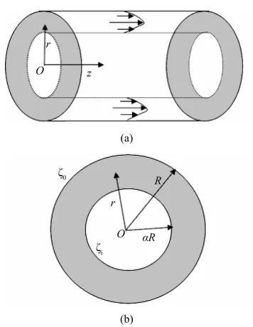
ter, i.e., is shown in Figure 1. The electrolyte fluid is acted upon by an axial (along z-direction) steady electric field of strength E0. The chemical interaction of electrolyte liquid and solid wall generates an EDL, a very thin charged liquid layer at the solid-liquid interface. A cylindrical coordinate system is adopted. In this theoretical model, the channel wall is assumed to be uniformly charged so that the electrical potential in the EDL varies in the r direction only and do not depend on
θ. For a symmetric binary electrolyte solution, assuming the electrical potential ψ of the EDL is steady, and its distribution and the local volumetric net charge density are described by the Poisson-Boltzmann equa- tions
LR
r, , z
e r
d 1 d , d d e r rr r r
r (1)
0
0 0
2 sinh v
e v
b z e r r n z e
k T
,
(2) here ε is the dielectric constant of the electrolyte liquid, n0 is the ion density of bulk liquid, zν is the valence, e0 is the electron charge, kb is the Boltzmann constant, and T is the absolute temperature. Substituting Equation (2) into Equation (1), the electrical potential in the annulus region can be expressed as
0 0 0
d 2 1 d sinh , d d v v b
r n z e z e
r
r r r k T
r (3) which is subject to the following boundary conditions
(a)
(b)
Figure 1. (a) Sketch of transient electro-osmotic flow through a microannulus along z direction; (b) Cross section of the microannulus.
o
, at r R , (4a) ,
i
at rR, (4b) where the ςo is the outer capillary wall zeta potential and the ςi is the inner capillary wall zeta potential. For sim- plicity, the following dimension dimensionless groups are introduced
0
1 2 2 2
0 0 0 0
, , ,
2
, ,
v
b
v v v
o o i i
b b
z e r
r K R
R k T
n z e z e z e
k T k T k T
, b (5)
Here κ is the Debye-Hückel parameter and 1/κ denotes the thickness of the EDL, and K is called the non-di- mensional electrokinetic width. The dimensionless elec- trical potential Equation (3) and the corresponding boundary condition (4) can be written as
21 d d sinh , d r d K
r r r
(6)
,
o
at r1, (7a)
,
i
at r. (7b) Assuming the electrical potential is small enough, the Debye-Hückel linearization approximation can be used for the hyperbolic sine function appearing in the right hand side of Equation (6), which means physically that the electrical potential is small compared with the ther- mal energy of the charged species. Equation (6) can be simplified as
2
1 d d . d r d K
r r r
(8) Equation (8) is a modified Bessel equation, and its so- lution has the following form
1 0 1 0 ,
A I Kr B K Kr
(9) where I0 and K0 is the modified Bessel functions of first and second kinds of order zero, respectively. Substituting boundary conditions of Equation (7) into Equation (9), the constants of A1 and B1 can be determined as
0 0 10 0 0 0
0 0
1
0 0 0 0
,
,
o i
o i
K K K K
A
K K I K K K I K
I K I K
B
K K I K K K I K
(10)
here i o is defined as the ratio of the zeta poten- tials of the inner wall to the outer wall of the annulus. Substituting Equation (10) into Equation (9), the final electrical potential can be expressed as
0 0 ,
o AI Kr BK Kr
[image:2.595.83.261.470.700.2]and the constants A and B are
0 K K A 00 0 0 0
0 0
0 0 0 0
,
. K K
K K I K K K I K
I K I K
B
K K I K K K I K
(12)
2.2. Velocity Distribution
electric field, the equation
In the presence of the applied
of the motion through the annulus due to electro-osmosis is given by the Navier-Stokes equation
0, e r E
t r r r z
(13)
Here ρ is the fluid density, is the axial velo- ci
, at (14a) ,
, 1 ,
u r t r u r t p
, u r t with zty component, which is along -direction, μ is the fluid viscosity, p is pressure, and E0 is constant electric field of strength. In fact, we have assumed that the time- dependent EOF does not affect the charge distribution in the Debye layer in Equation (13). Generally, the transient effect of EDL relaxation can be neglected because the time scale related to electro migration in the EDL is at least two orders smaller that the characteristic time asso- ciated with the evolution of the EOF [19]. The boundary conditions of Equation (13) are supposed no slip and can be written as
, 0u r t r R ,
, 0u r t at rR. (14b) It is important to mention that th
di
here e boundary con- tions at the walls may exhibit apparent slip behavior instead of following the classical no-slip conjecture. Such deviations, not being the focal point of concern in the present study, are not considered here. Introducing the following dimensionless groups:
0 2
0
, u ,
t t u u ,
,
b s
s v
s
E k T
u z e
R
p z z
z
u RL L
(15)
where is the normalized pressure gradient applied e
along th channel axis.
Using Equations (2) and (8), for small zeta potential, the Equation (13) can be normalized as
2
1
u u
r K .
t r r r
(16) The normalized boundary conditions Equation (14) are
,
0,u r t at r 1, (17a)
,
0u r t , at r .
Let us employ the metho Lapla fine
(17b)
d of ce transform de- d by
r s, L u r t
,
0u r t
,
e d .t (18) If initial condition satisfiesst
U
,0 0u r , t
trans 7) give
hen the forms of Equations (16) and (1
2 2
, 1 ,
U r s U r s
2
, 1
sU r
s
r r
r
K
s s
(19)
, 0U r s , at r 1, (20a)
, 0U r s , at r .
Substituting Equatio into
(20b) n (11) Equation (19), we have
2 0 0 1 . o r r r 2 2, 1 , ,
U r s U r s
sU r s
K AI Kr BK Kr
s s
(21)
Equation (21) is linear and inhomogeneous ordinary differential equation, and its solution can be expressed by the sum of a general solution U r sh
, correspondingto homogeneous equation and a special solution
,s U r s
, h
, s
, 2U r s U r s U r s .
s
(22) The homogeneous solution of Equation (21) is written as
, 0
0
,h
U r s EI sr FK sr (23) here E and F are constants, which can be determined from boundary conditions of Equation (23). Considering the formation of the right hand side of Equation (21), the special solution can be expressed as
, 0
0
,s
U r s CI Kr DK Kr (24) here C and D are constants. Substituting Equation (24) into Equation (21) yields
2 0 0 0 2 2 0 0 0 2 2 0 0d 1 d d d
d 1d d d
1 ,
o
I Kr I Kr
C sI
r r
r
K Kr K Kr
D s
r r
r
K AI Kr BK Kr
Kr K Kr s (25)
From Equation (8), we can obtain easily
2
0 0 2
0 2
2
0 0 2
0 2
d 1d ,
d d
d 1d .
d d
I Kr I Kr
K I Kr
r r
r
K Kr K Kr
K K Kr
r r
r
Substituting Equation (26) into Equation (25) and equalizing the coefficients in front of the modified Bessel functions I0 and K at the two sides of the equati
0 0
0 0 2
,
.
U r s
EI sr FK sr
CI Kr DK Kr s
(28) on yields
0
2 2
2 , 2 .
o o
AK BK
C D
s s K s s K
(27)
Inserting Equations (23) and (24) into Equation (22),
the solution of velocity U r s
, is determine the constants E and F as Using boundary conditions of Equation (20), we can
2 2
0 0 0 0 0 0
0 0
,
K s CI K s K s CI K DK K s
E
s I s K s
(29)
DK K
0 0
I s K
2 2
0 0 0 0 0 0
0 0 0 0
.
I s CI K DK K s I s CI K DK K s
F
I s K s I s K s
(30)
Now the analytical solution of Laplace transform of EOF velocity through a microannular can be determined by Equation (28) with related constants given by Equa- tions (12), (27), (29) and (30). Then using the method of
rse Laplace transform defined by
where is a vertical line to the right of all singularities of U r s
,f the ex
in the complex s plane. Due to ity o press of
the complex-
,U r s , the exact so
EOF y can not be obtained analytically. Therefore, the numerical computation must be performed by nu-
e anal
express
lution of the velocit
merical inverse Laplace transform [20].
Th ytical solution of Newtonian fluid velocity in the steady state can be ed as
inve
1, ,
1 , d , 2π
st u r t L U r s
U r s e s i
(31)
2
0
,t r 4oAI K
where,
u r r BK Kr0 C1lnr C 2 (32)
2
1 4 o 0 0 l
C AI K BK K C2 n , (33)
2
C 4oAI K0 BK K0 (34)
3. Results and Discussions
In the previous section, dimensionless transient velocity depend mainly on the ele
inner to outer radius ratio α, inner to outer zeta potential re gradient Ω. In this ce of these parameters
ta potential ra
deter- mined by electrical potential is
the EDL, appreciable reducti
to occur outside the EDL. In addition, with the increase Larger β leads to larger velocity near the inner microan- nulus wall. The reason is that the electric force
mainly concentrated in ons in velocity are observed
EOF ctrokinetic width K, ratio β and the normalized pressu
section, we will discuss the influen
on the dimensionless transient EOF velocity.
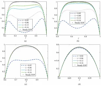
For fixed α = 0.4, Figure2 illustrates the variations of normalized EOF velocity at different time (0.02, 0.06, 0.12 and 0.20) with radius for different inner to outer zeta potential ratio β (−1, 0, 1 and 2). It can be seen from
Figure 2 that for negative inner to outer ze
tio β (see Figure 2(a)), the directions of the EOF ve- locity near EDL of two microannulus wall are inverse. However, for positive inner to outer zeta potential ratio β
(see Figures 2(b)-(d)), the directions of the EOF veloc- ity within the whole gap of the microannulus are uniform.
of time, the EOF velocity approaches gradually steady status. That is to say, further increase of the time will lead to invariable velocity profile.
For fixed β = 1, Figure 3 shows the variations of nor- malized EOF velocity at different time with radius for different inner to outer radius ratio α (0.2, 0.4, 0.6 and 0.8). Similarly, with the increase of time, the EOF veloc- ity approaches gradually steady status. In addition, with the increase of inner to outer radius ratio α, the gap be- tween the two walls of microannulus becomes small, thus the time needed to attain the steady status become small. The velocity profile changes from plug-like to parabo- lic-like shape.
K20, 0 4,. o 1, 0
[image:5.595.129.464.85.368.2]
Figure 2. Variations of normalized EOF velocity at different time with radius for different . (a) β = −1; (b) β = 0; (c) β = 1; (d) β = 2.
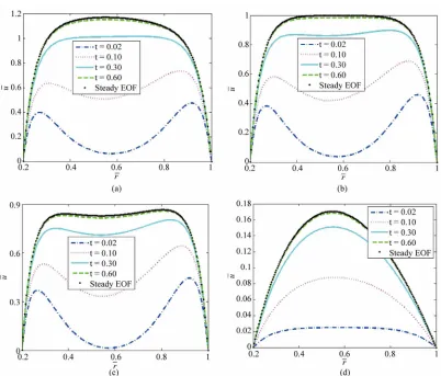
K20, 1, o 1, 0
[image:5.595.127.471.411.704.2]Figure 4. Variations of normalized EOF velocity at different time with normalized pressure driven flow (K = 20, α = 0.2). (a) ; (b) 0, 1,o1; (c) 2, 1,o1; (d) 2, 0,o0.
2, 1, o 1
increase. So the dimensionless velocity amplitude in- creases. In addition, with the increase of time, the EOF velocity approaches gradually steady status. Figure4(d)
depicts the flow of the fluids only under pressure-driven, i.e., no external electroosmotic flow, equivalent to Poi- seuille flow.
Under the different dimensionless parameters, Figures 2-4 respectively compared the numerical solution with the analytical solution in steady state. As can be seen in the Figures 2-4, they are essentially coincident.
4. Conclusions
A semi-analytical solution of the transient mixed EOF/ PDF of Newtonian fluids through a microannulus under the Debye-Hückel approximation is presented in this work. The solution involves analytically solving the lin- earized Poisson-Boltzmann equation and Navier-Stokes equation. The results show that the velocity profiles de- pend greatly on the non-dimensional electrokinetic width K, the inner to outer radius ratio α, the inner to outer wall zeta potential ratio β and the normalized pressure gradi- ent Ω. With the numerical computation of inverse La-
place transform, the following conclusions are drawn: 1) The inner to outer wall zeta potential ratio β deter- mines the direction and magnitude of EOF velocity. Negative β leads to the inverse directions of the EOF velocity near EDL of two microannulus wall and vice versa. Larger β leads to larger velocity near the inner microannulus wall.
2) With the increase of inner to outer radius ratio α, the time needed to attain the steady status become less.
3) For a given dimensionless time, along with the di- mensionless pressure gradient increased, velocity ampli- tude section becomes bigger.
The transient evolution of the velocity profiles pro- vides a detail insight of the flow characteristic of this flow configuration.
5. Acknowledgements
[10] S. Arulanandam and D. Li, “Liquid Transport in Rectan-gular Microchannels by Electroosmotic Pumping,” Col-loids and Surfaces A: Physicochemical and Engineering Aspects, Vol. 161, No. 1, 2000, pp. 89-102.
doi:10.1016/S0927-7757(99)00328-3 omous Region (Grant No. NJYT-13-A02), the Natural
Science Foundation of Inner Mongolia (Grant Nos.: 2010BS0107, 2012MS0107), the research start up fund for excellent talents at Inner Mongolia University (Grant No.: Z20080211) and the support of Natural Science Key Fund of Inner Mongolia (Grant No: 2009ZD01), the In- novative programs funded projects of Postgraduate Edu- cation in Inner Mongolia Autonomous Region, and Inner Mongolia University of enhancing the comprehensive strength funding (Grant No. 1402020201).
REFERENCES
[1] H. A. Stone, A. D. Stroock and A. Ajdar, “Engineering Flows in Small Devices: Microfluidics toward a Lab-On- a-Chip,” Annual Review of Fluid Mechanics, Vol. 36, No. 1, 2004, pp. 381-411.
doi:10.1146/annurev.fluid.36.050802.122124
[11] F. Bianchi, R. Ferrigno and H. H. Girault, “Finite Ele-ment Simulation of an Electroosmotic Driven Flow Divi-sion at a t-Junction of Microscale DimenDivi-sions,” Analyti-cal Chemistry, Vol. 72, No. 9, 2000, pp. 1987-1993. doi:10.1021/ac991225z
[12] C. Y. Wang, Y. H. Liu and C. C. Chang, “Analytical So- lution of Electroosmotic Flow in a Semicircular Micro-channel,” Physical of Fluids, Vol. 20, No. 6, 2008, Arti-cle ID: 063105. doi:10.1063/1.2939399
[13] P. Dutta and A. Beskok, “Analytical Solution of Time Periodic Electroosmotic Flows: Analogies to Stokes’s Econd Problem,” Analytical Chemistry, Vol. 73, No. 21, 2001, pp. 5097-5102. doi:10.1021/ac015546y
[14] X. M. Wang, B. Chen and J. K. Wu, “A Semianalytical Solution of Periodical Electro-Osmosis in a Rectangular Microchannel,” Physical of Fluids, Vol. 19, No. 12, 2007, Article ID: 127101. doi:10.1063/1.2784532
[2] R. J. Hunter, “Zeta Potential in Colloid Science,” Aca- demic Press, San Diego, 1981.
[3] G. Karniadakis, A. Beskok and N. Aluru, “Micorflows and Nanoflows: Fundamentals and Simulation,” Springer, New York, 2005.
[4] D. Burgreen and F. R. Nakache, “Electrokinetic Flow in Ultrafine Capillary Slits,” The Journal of Physical Che- mistry, Vol. 68, No. 5, 1964, pp. 1084-1091.
[5] S. Levine, J. R. Marriott, G. Neale and N. Epstein, “The- ory of Electrokinetic Flow in Fine Cylindrical Capillaries at High Zeta-Potentials,” The Journal of Physical Che- mistry, Vol. 52, No. 1, 1975, pp. 136-149.
The Journal ical Chemistry, Vol. 225, No. 1, 2000, pp. 247-250.
Flow through an Elliptical Microchannel: Ef-
nels with ffects,” International Journal of Heat and
ol. 41, No. 24, 1998, pp. 4229-4249.
[15] S. Chakraborty and S. Ray, “Mass Flow-Rate Control through Time Periodic Electro-Osmotic Flows in Circular Microchannels,” Physical of Fluids, Vol. 20, No. 8, 2008, Article ID: 083602. doi:10.1063/1.2949306
[16] Y. J. Jian, L. G. Yang and Q. S. Liu. “Time Periodic Ele- ctro-Osmotic Flow through a Microannulus,” Physical of Fluids, Vol. 22, No. 4, 2010, Article ID: 042001. doi:10.1063/1.3358473
[17] H. J. Keh and H. C. Tseng, “Transient Electroki tic Flow in Fine Capillaries,” Journal Colloid Interface Science,
i:10.1006/jcis.2001.7797 [6] H. K. Tsao, “Electroosmotic Flow through an Annulus,”
of Phys
[7] Y. J. Kang, C. Yang and X. Y. Huang, “Electroosmotic Flow in a Capillary Annulus with High Zeta Potentials,” The Journal of Physical Chemistry, Vol. 253, No. 1, 2002, pp. 285-294.
[8] J. P. Hsu, C. Y. Kao, S. J. Tseng and C. J. Chen, “Elec- trokinetic
fects of Aspect Ratio and Electrical Boundary Condi- tions,” The Journal of Physical Chemistry, Vol. 248, No. 1, 2002, pp. 176-184.
[9] C. Yang, D. Li and J. H. Masliyah, “Modeling Forced Liquid Convection in Rectangular Microchan
Electrokinetic E Mass Transfer, V
doi:10.1016/S0017-9310(98)00125-2
ne
Vol. 242, No. 2, 2001, pp. 450-459. do
[18] Y. J. Kang, C. Yang and X. Y. Huang, “Dynamic Aspects ,” of Electroosmotic Flow in a Cylindrical Microcapillary International Journal of Engineering Science, Vol. 40, No. 20, 2002, pp. 2203-2221.
doi:10.1016/S0020-7225(02)00143-X
[19] C. C. Chang and C. Y. Wang, “Starting Electro-Osmotic Flow in an Annulus and in a Rectangular Channel,” Elec-trophoresis, Vol. 29, No. 14, 2008, pp. 2970-2979. doi:10.1002/elps.200800041
[2
Tran- 0] F. R. De Hoog, J. H. Knight and A. N. Stokes, “An
Im-proved Method for Numerical Inversion of Laplace sforms,” SIAM Journal on Scientific and Statistical Com- puting, Vol. 3, No. 3, 1982, pp. 357-366.