All Pay Auctions with Polynomial Rewards

Munich Personal RePEc Archive

All-Pay Auctions with Polynomial

Rewards

Bos, Olivier and Ranger, Martin

University Panthéon-Assas (Paris 2), University of Bonn

11 May 2013

Online at

https://mpra.ub.uni-muenchen.de/47587/

All-Pay Auctions with Polynomial Rewards

Olivier Bos†

University Panth´eon-Assas (Paris 2)

Martin Ranger‡

University of Bonn

This version: May, 2013

Abstract

This paper examines a perfectly discriminating contest (all-pay auction) with two asymmetric players. We focus on unordered valuations. Valuations are endogenous (poly-nomial functions) and depend on the effort each player invests in the contest. The shape of the valuation function is common knowledge and differs between the contestants. Some key properties of R&D races, lobbying activity and sport contests are captured by this framework. After analyzing the unique mixed strategy equilibrium, we derive a closed form of the expected expenditure of both players. We characterize the expected expendi-ture by means of incomplete Beta functions.

Keywords: All-pay auctions, contests

JEL Classification: D44, D72

∗_{A previous version of this paper circulated under the title “All-pay auctions with endogenous rewards”. The} first author thanks the University of Bonn and CORE (Universit´e Catholique de Louvain) for their hospitality and acknowledges financial support from the European Commission (Marie-Curie Fellowship). We would like to thank Atsu Amegashie, Raouf Boucekkine, Subhasish Chowdhury, Gabrielle Demange, Aner Sela and Ron Siegel for their valuable comments, discussions and remarks. We also thank two anonymous referees for their valuable comments. All remaining errors are ours.

†_{Corresponding author. University Panth´eon-Assas (Paris 2), LEMMA, 5/7 avenue Vavin, 75006 Paris,} France. E-mail: [email protected].

1

Introduction

Although commonly assumed to be fixed, the size of the prize in a contest may in fact be endogenous and depend on the effort made by the contestants. In particular, a higher level of effort may lead to higher valuations.1 In other words, the effort expended in a contest may increase both the probability of winningand the size of the prize. Moreover, contestants may differ with respect to the magnitude of this effect, and the same effort levels may lead to a different valuation of winning the contest (Kaplan, Luski, Sela, and Wettstein,2002).

Such an environment is descriptive of several economic issues. In R&D races, for example, an increase in the amount of resources spent on developing new technologies may result in a shorter product pipeline and in the firm winning the race. At the same time, the additional resources may improve the quality of the final product and therefore its market value. Asymmetric market structures and differences in marketing, existing product variety or spill-over effects to related research projects are likely to lead to differences in the marginal value of R&D spending. Organizational differences in research departments or a different composition of inputs into the research process may likewise lead to different values of winning the race. In some sense, academic hiring efforts may follow a similar pattern. As long as universities attempt to attract faculty by offering productivity enhancing inducements, such as research funds, expanded seminar series or access to data sets, they are likely to increase the productivity of the potential new hire and at the same time the value of being able to hire the desired candidate.

In the classical example of a lobbying contest, the value of the legislation enacted or the project awarded may depend on the magnitude of the contribution to the political institution involved. Asymmetries may enter the contest through the pre-existing political connection of the lobbyist, so that an organization with conservative credentials would obtain a more favourable outcome with a conservative government than a more liberal lobbyist. Lastly, in professional sports, the effort invested by a team increases its expected score making a win more likely. In addition, conditional on having won the game, a higher score may raise the reputation of the team. For teams quoted on the stock market, such as several European soc-cer teams, this may translate into additional stock price gains.2 Again, differences between teams may lead to asymmetries in this effect.

This paper examines the equilibrium of a contest with endogenous rewards and derives the aggregate expenditure of the contestants – which is the main contribution of the paper. Indeed, it is useful for the organizer of the contest to know the expected aggregate expenditures if he would like to maximize it and then to affect the design of the contest. It might be the case

1

Higher effort levels can also lead to a lower value of winning a contest. In a war of attrition, for example, the effort spent to win is likely to make the winner more vulnerable in future conflicts and contestants prefer to win at lower effort levels.

2

in R&D races. We examine a contest modeled as an all-pay auction, that is a situation in which the contestant investing the largest effort will win with certainty. Regardless of whether they won or not, all contestants have to pay their effort cost. Information is assumed to be complete and valuations are asymmetric and endogenous (polynomial functions). For simplicity, the analysis is limited to two participants. The payoff from winning the contest, that is the valuation less the cost of effort, is assumed to decline strictly in effort despite valuations that increase in the invested effort. Similar to traditional all-pay auctions, the participants in the contest thus prefer to win at lower effort levels. This assumption contrasts withAmegashie (2001) who investigates situations where the returns to additional expenditures in all-pay auctions exceed the costs and players therefore could aim to win with higher efforts. Contrary to the case where payoffs strictly decrease he finds that a Nash equilibrium in pure strategies exists.

A second related paper is Kaplan, Luski, and Wettstein(2003), who investigate a model of innovation and R&D races with a structure similar to an all-pay auction. Information is complete, values and innovation cost are time dependent and firms compete in when to bring the innovation to the market. In consequence, the usual equivalence of staying out of the contest and exercising zero effort does not apply. In contrast to our paper, a closed form solution for expected aggregate expenditure is not given. Siegel (2009, 2010) also studies all-pay auctions with complete information and non-ordered contestants. The differences are in the levels of generality. Whereas Siegel’s broad approach covers quite general model specifications – in particular he focuses on contests where all-pay auction is a sub-class of contests – our more specific set-up allows us to determine a closed form solution for expected equilibrium expenditures thanks to the incomplete Beta functions.3 This result could be useful for applications of contests with – polynomial – endogenous rewards as in R&D races. Three other recent papers with complete information are also related to our work. In-terestingly, Chowdhury (2009) investigates the two contestants all-pay auction with winning payoffs as non-monotonic functions of their own efforts. He finds conditions under which a pure strategy Nash equilibrium exists and determines the unique mixed strategy Nash equi-librium. Furthermore,Siegel (2012) generalizes the results of Siegel(2009) forn contestants to a model with non-monotonic payoff functions. Sacco and Schumtzler (2008) characterize pure and mixed strategies Nash equilibria with contestants’ valuation as a function of both own and rival efforts. In addition to their theoretical results they focus on an experimental analysis. Yet, as the other papers with complete information these do not provide a closed form solution for expected equilibrium expenditures.

A related paper with incomplete information isKaplan, Luski, Sela, and Wettstein(2002) who investigate an all-pay auction where the rewards are additively or multiplicatively

sepa-3_{Siegel(2010) provides an algorithm to solve equilibrium expenditures in the general framework ofSiegel}

rable in the type of the players. This setting seems well-suited to R&D races, political contest or lobbying activities. Kaplan, Luski, Sela, and Wettstein(2002) solve for the equilibrium bid function and link the size of the reward as well as the costs of bidding to the expected sum of equilibrium bids. Cohen, Kaplan, and Sela(2009) study an all-pay auction with additively and multiplicatively separable rewards under incomplete information where the designer can set the shape of the reward function. In particular, they determine that the optimal additively separable reward is not necessarily positive. In our model, we investigate additively separable rewards with complete information.

The next section introduces the model. While valuations are not ordered, they are regular in the sense that over some range of effort one player has higher valuations while above a certain threshold effort level the valuations of the other player are higher. The existence of a Nash equilibrium in mixed strategies and equilibrium effort levels are derived in Section 3. A closed form solution for the aggregate expected equilibrium expenditure is derived in Section 4– this is indeed the main contribution of this paper.

2

The Model

Consider two players or group of players, i= 1,2 who choose effort levelsxi ∈R+

simultane-ously and independently in a contest. The shape of their valuations is given byVi(·) :R+→R

which specifies the size of the prize as a function of their effort. The valuation of winning the contestVi for eachi= 1,2 consists of a common elementvand the additive polynomial

func-tion βixαii with 0< βi <1 and αi ≥1. The shape of every player’s valuation – the constant

v and parameters αi and βi – are common knowledge at the beginning of the contest. Both

players pay their effort cost and final payoffs for each player i= 1,2 are given by

ui(xi, xj) =

   

  

v+βixα_ii−xi ifxi> xj

v+βixα_ii

2 −xi ifxi=xj

−xi ifxi< xj

In an all-pay auction bidders have to pay their effort independently of the outcome of the contest and only the winner keeps a balance from his effort spent (unlikely to the first-price auction with complete information for example). The following assumption captures this element.

Assumption 1 (A1). The winning payoff is strictly decreasing with the effort spent.

AssumptionA1makes the contestants prefer winning at lower effort levels. In other words, the net payoff from an additional unit of effort is negative and then βiαixαi−1 < 1 for all

x∈[0,x˜] where ˜x is the maximum effort such as assumptionA1is satisfied. Remark that ˜x

more specific thanSiegel(2009,2010) – it is actually a special case of their model – it allows us to determine a closed form of the aggregate expected equilibrium expenditure (which is not possible in Siegel (2009, 2010)).4 _{Moreover, the shape of the valuations can be derived}

because of an axiomatization.5

The case where Vi(xi) = v for all xi corresponds to a pure common value setting. It is

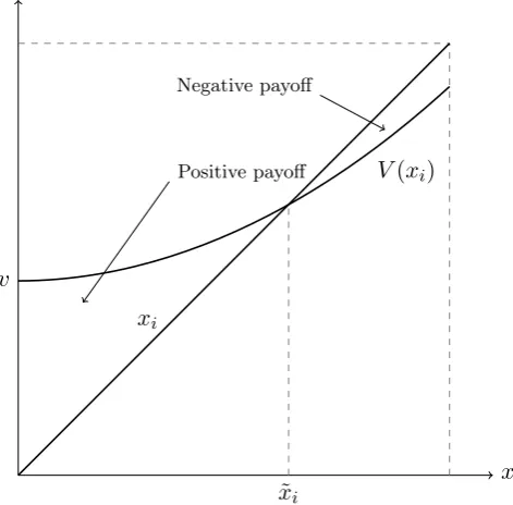
well-known that under these circumstances there is no Nash equilibrium in pure strategies. As Amegashie (2001) has shown, if utility is not monotonically decreasing in effort, a pure strategy Nash equilibrium exists. Although his framework is different, the link between in-creasing utility and equilibrium existence is likely to apply to our set-up as well. The reward components of the all-pay auction are depicted in Figure 1.

As valuations are dependent on the effort of the two contestants, they need not to be ordered. In other words, for two different effort levels, the ranking of the valuations could

be reversed. If αi > αj, for example, Vj(x) > Vi(x) for all x <

_β

j

βi

1

αi−_αj

and Vj(x) ≤

Vi(x) otherwise. Non-ordered valuations seem well-suited for the real-world applications that

motivate our analysis. Indeed, with different marginal returns to effort in R&D races, lobbying or sports contests, the ranking of the valuations depends on effort levels and valuations are unlikely to be ordered.6

4

Siegel(2009,2010) do not specify the shape of the valuation and cost functions. Yet Siegel(2009,2010) also use a similar assumption to assumptionA1.

5

Let us denote ei(.) a differentiable and continuous functions such asVi(.) =v+ei(.). Given the three

following assumptions

• ei(.) is a non-negative and increasing function for allxi>0 andei(0) = 0

• contestants prefer winning at lower effort levels (which is equivalent to our assumptionA1) • ei(.) is a homogeneous function

the shape ofei(.) is our polynomial function. Details and economic interpretations are available in a previous

draft of this paper,Bos and Ranger(2009).

6

xi

v

˜

xi

V(xi)

xi

Positive payoff Negative payoff

Figure 1: Payoff of Winning

3

Equilibrium Characterization

It is a well known result that all-pay auctions with constant heterogeneous valuations, that is valuations that are independent of the submitted bids, have a unique equilibrium in mixed strategies (Hillman and Riley (1989), Baye, Kovenock, and de Vries (1996) for linear costs, Che and Gale (1998), Che and Gale (2006), Kaplan and Wettstein (2006) and Vartiainen (2007) for non-linear cost functions). In recent papers,Siegel(2009,2010,2012) extends this result to non-ordered contestants in a general framework.

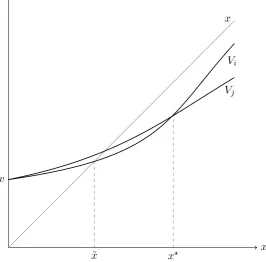
To simplify the notation we define the “weak” and the “strong” player and denote them by the subscripts w and s, respectively. The intuition is simple: since payoffs are falling in effort by assumption A1 there will be a level of effort after which the payoff obtained will be negative even if the contest is won. The “weak” player determines the maximum effort any player is willing to exercise in the contest. At this effort level its utility from winning the contest is zero; the “strong” player, in contrast, still obtains a positive payoff at the same effort level. Non-ordered valuations and ordered valuations are depicted in Figure4and Figure5 in Appendix C.

Definition 1. A player is called “weak” if he determines the maximum effortx˜in the contest, that isv+βwx˜αw−x˜= 0 and v+βsx˜αs−x >˜ 0. His opponent is called the “strong” player.

Let us consider αi > αj. If ˜x is such as v+βjx˜αj −x˜ = 0 and ˜x >

_β

j

βi

1

αi−_αj

the player i is the “strong” player. Otherwise, the player j is the “strong” player and the maximum effort is given by ˜xsuch asv+βix˜αi−x˜= 0. Unlike in a standard all-pay auction,

it is not enough for a particular player to have the higher valuation over an interval of x

in order to be the “strong” player. Rather, the relative strength of a player is determined not only by the difference between the valuations at a particularx but also – implicitly – by

the distance from the thresholdβj

βi

1

αi−_αj

which defines the order of the valuations on each sub-interval.

It follows from the implicit function theorem that the maximum effort is increasing inβw,

decreasing inαw if ˜x <1 and increasing inαw if ˜x >1,

dx˜

dβw

= x˜

αw

1−βwαwx˜αw−1

>0 and dx˜

dαw

= βwx˜

αw_{ln ˜x}

1−βwαwx˜αw−1

  

 

<0 if ˜x <1 = 0 if ˜x= 1

>0 if ˜x >1

  

 

(1)

The signs follow from assumption A1.

Define the mixed strategies at the equilibrium by Fi(·) = P(X ≤ ·) for both players

i=s, w. The following proposition determines the unique Nash equilibrium strategies for the two players and the corresponding equilibrium payoffs.

Proposition 1.The unique Nash equilibrium is in mixed strategies as follows. Players choose their effort randomly according to the cumulative distributions functions

Fs(x) =

x v+βwxαw

for all x∈[0,x˜]

Fw(x) =

v+βsx˜αs −x˜+x

v+βsxαs

for allx∈[0,x˜]

And the expected equilibrium payoffs are

u⋆_s=βsx˜αs−βwx˜αw

u⋆_w= 0

Proof. Let us define ˜vi(x) =v+βixαi−x and ˜ci(x) =x. Then, the bidders’ expected utility

could be written asFi(x)˜vi(x)−(1−Fi(x))˜ci(x). Observe that ˜vi and−˜ci are continuous and

strictly decreasing, ˜vi(0) =vand limx→+∞˜vi(x)<0 and ˜v−s1(0)>˜v−w1(0) = ˜x. Consequently

all assumptions ofSiegel (2010) are satisfied. In addition what he called the threshold T of the contest is in our case the maximum effort ˜x of the “weak” bidder. Thus, Theoreom 3 of Siegel(2010) can be applied and our result follows.

Corollary 1. The expected equilibrium payoff of the “strong” player is (i) decreasing in βw

and (ii) decreasing in αw if x >˜ 1 and increasing otherwise.

Proof. See Appendix A.

This asymmetry in the parameter effects is interesting for its implications. As the payoff of the “strong” player is given by βsx˜αs −βwx˜αw the impact of the reward parameters βw

and αw comes from two sources. On one hand we can identify a parameter effect from the

endogenous valuation of the “weak” player independent of the effort level, in which a higher

βw (respectively a smaller αw if ˜x <1 and a higher one if ˜x >1) reduces the payoff of the

“strong” player independent of the effort levels. The maximum effect, on the other hand, works through the impact of the relative values of βw and αw on ˜x. If the maximum effect

and theparameter effect have contradictory signs, the latter dominates.

It is possible to compare the (standard) all-pay auction with exogenous valuationsVi(x) =

vi and our setup whereVi(x) =v+βixαi.7 Even if rewards lead to either a higher or a lower

valuation than in the standard case of all-pay auction, it is convenient to assume that the maximum effort is the same in the endogeneous and standard all-pay auctions. Indeed, the maximum effort could be decided ex ante, for example as a limit of the expenditure in an R&D race. In consequence, in the standard all-pay auction valuations are ordered and the “weak” contestant is the one with the lowest valuation. She determines her maximum effort equal to her valuation vw such that vw = ˜x = v+βwx˜αw. Then, vs, the valuation of the

“strong” contestant is superior tov+βwx˜αw.

Corollary 2. The expected equilibrium payoff of the “strong” player in the all-pay auction with polynomial rewards is lower than in a standard all-pay auction if and only if her valuation

vs is superior to v+βsx˜αs.

This result comes from the comparison of the players’ expected equilibrium payoff given by Proposition1 and the contestants’ expected equilibrium payoff given by Hillman and Riley (1989) and Baye, Kovenock, and de Vries (1996) in the standard all-pay auction which is

vs−vw for the “strong” player.

4

Aggregate Expenditures

We now derive an explicit expression for the expected equilibrium expenditure of both con-testants by means of the incomplete Beta functions. We present a very short overview of the family of incomplete Beta functions which are a useful tool for the computations of the

7

The analysis does not change if the exogenous part of the valuationsviis not common to both contestants

expected revenues. The incomplete Beta functions belongs to the general class of hypergeo-metric functions and are studied in detailSpanier and Oldham (1987) Chapter 58 (see also Temme(1996) for a more recent textbook).8

Definition 2. The incomplete Beta function, B(ν, µ, x), with 0 ≤ x ≤ 1, µ ∈ R_{, ν > 0, is}

given by the Euler integral representation:

B(ν, µ, x) =

Z x

0

tν−1

(1−t)1−µdt

Theorem 1. The incomplete Beta function, B(ν, µ, x), with 0 ≤ x < 1, µ ∈ R, ν > 0, is given by the expansion series:

B(ν, µ, x) = (1−x)

µ

ν

∞

X

j=0

(µ+ν)j

(1 +ν)j

xj+ν

where (y)n denotes the Pochhammer symbol such that

(y)n=

Γ(j+y) Γ(y) ,

where Γ(.) is the special function Gamma.

Proposition 2. The aggregate expected equilibrium expenditures are given by

ERs=

       − v βw

1 + 1

βw

ln(1−βw)

ifαw = 1

˜

x− 1

αwvφ

2 αw B 2 αw

,1− 2

αw

, φx˜

αw

1 +φx˜αw

if αw>1

ERw =

      

1−βs

βs

ln(1 +ϕx˜)

˜

x+ v

βs

−x˜

if αs= 1

˜

x− 1

αsvϕ

2 αs B 2 αs

,1− 2

αs

, ϕx˜

αs

1 +ϕx˜αs

−βsx˜

αs_−β

wx˜αw

αsv2ϕ

1 αs B 1 αs

,1− 1

αs

, ϕx˜

αs

1 +ϕx˜αs

if αs>1

withx˜=v+βwx˜αw, ϕ= β_vs and φ= β_vw.

Proof. See Appendix A.

The Euler integral form of the incomplete Beta functions is used in the proof to identify it. An explicit form of the expected revenues are given in Appendix A by the means of the expansion series of the incomplete Beta functions.

Assuming a linear relationship between effort and the valuations, αs =αw = 1, one can

simplify the expression forE_{Rw to}

E_{Rw =} 1−βs

1−βw

v βs

−1 +

1−βw+βs

βs

ln

βs

1−βw

+ 1

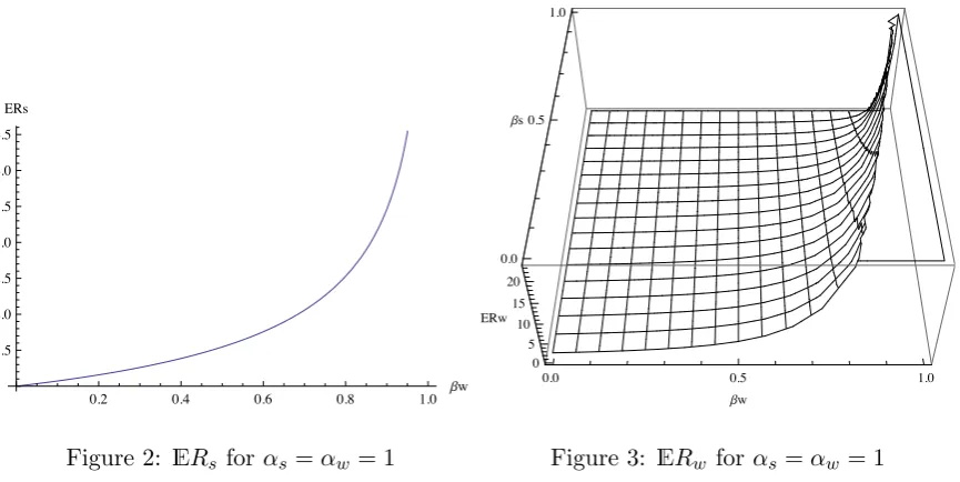
The relationship between the expected equilibrium expenditure for both players and the val-ues forβw and βs can be shown graphically (Figure2 and Figure3 withv= 2).

0.2 0.4 0.6 0.8 1.0 Β

w 1.5

2.0 2.5 3.0 3.5 4.0 4.5 ERs

Figure 2: ERs forαs=αw = 1

0.0 0.5 1.0

Βw 0.0

0.5 1.0

Βs

0 5 10 15 20

ERw

Figure 3: ERw forαs=αw = 1

The features of the individual expenditures that we observe in graphs 2 and 3 can be extended to all values ofαsandαw. It is thus possible to compare the standard all-pay auction

with exogenous valuationsVi(x) =vi with our setup where Vi(x) =v+βixαi. Qualitatively,

βi and αi (when ˜x > 1) play the same role as vi in the standard framework and αi (when

˜

x≤1) the inverse one and the results should comparatively similar with respect to individual expected equilibrium expenditure. The following corollary confirms this intuition for all value ofαs, αw, βs, βw and v.

Corollary 3. The individual expected equilibrium expenditures

(i) of the “strong” player are increasing in βw and decreasing in αw if x˜≤1.

(ii) of the “strong” player are independent of βs and αs.

(iii) of the “weak” player are decreasing in βs, increasing in αs if x˜≤1.

(iv) of the “weak” player are increasing in βw, decreasing in αw if x˜≤1 and increasing in

αw if x >˜ 1.

We are not able to compute the sign of the derivatives of the role of the parametersαs on

the “weak” player’s andαw on the “strong” player’s expected equilibrium expenditure when

˜

x >1. Yet, we did not find any example which could contradict the intuition given above. These results (Corollary 3) may have implications for the designer of a contest. If the designer is interested in eliciting the largest amount of effort, in cases where the effort accrues directly to him, and if he can manipulate the contest technology of both players, Corollary 3 indicates a method to achieve this goal. In addition, the contestants themselves have an incentive to influence the parameters in the valuation functions. A “weak” firm in an R&D race, for example, would prefer a larger value for βw and a smaller value for αw if ˜x ≤ 1

(respectively a higher value if ˜x >1) in order to decrease the expected equilibrium payoff of its competitor (see Corollary1). If the contestant can chose the parametersαi andβiat some

cost before the beginning of the contest, the game can be extended to include the pre-contest selection of the contest technology.

As in Section 3 for Corollary 2, we compare our setup where Vi(x) = v+βixαi with the

standard all-pay auction where the valuationvw of the “weak player” is such that vw= ˜x.

Corollary 4. The expected equilibrium expenditures of the “strong” player in the all-pay auction with polynomial rewards is lower than in the standard all-pay auction.

Proof. As vw > v+βwxαw for all effort inferior to ˜x, the “strong” player’s mixed strategy

in the contest with rewards is stochastically dominated by the one in the standard contest.

Then, the result follows from E_{Rs = ˜x}−

Z ˜x

0

Fs(x)dx.

The effect on the expected equilibrium expenditures of the “weak” contestant is not clear. Indeed, as the payoff of the “strong bidder” decreases if vs > v+βsx˜αs, the effect of the

reward on the mixed strategy of the “weak” contestant is ambiguous.

5

Conclusion

In this paper we examine a perfectly discriminating contest (all-pay auction) with two asym-metric players and polynomial valuations in a complete information environment. Similar to real-world situations, we postulate that the value of winning depends on the effort levels invested. In particular, we assume that higher effort levels lead to higher prizes but that this increase is smaller than the cost of effort. The contestants thus prefer to win at lower effort levels. We believe that this set-up captures the nature of many contests such as R&D races, lobbying games or sports events.

the lower effort limit. Within these limits, valuations need not be ordered, however, as (due to the asymmetry) both players may have the higher valuation at different levels of effort. This notwithstanding, we show that the equilibrium strategies and expected payoffs depend on the strength of the player.

In equilibrium, the expected equilibrium payoff of the “strong” player is positive and de-pends on the parameters of both players’ valuation function. In particular, it is decreasing in the steepness of the “weak” player’s valuations. We are able to characterize the expected expenditure thanks to the incomplete Beta functions. This result could be useful for applica-tions of contests with polynomial rewards as in R&D races. For example, the organizer of the contest could provide incentives to contestants such as they would select a contest technology (their parameters αi and βi) which would increase the expected aggregate expenditures.

Appendix A: Proofs

Proof of Corollary1. (i)

∂u⋆ s

∂βw

= dx˜

dβw

(βsαsx˜αs−1−βwαwx˜αw−1)

| {z }

maximum effect

− x˜αw

|{z}

parameter effect

(2)

= dx˜

dβw

βsαsx˜αs−1−1

(3)

<0 (4)

To arrive at equation (3) from (2) we apply the implicit function theorem to ˜x=v+βwx˜αw

in ˜xandβwsuch that

dx˜

dβw

1−βwαwx˜αw−1

= ˜xαw_{. The result then follows from assumption}

A1and (1).

(ii)

∂u⋆_s ∂αw

= dx˜

dαw

βsαsx˜αs−1−βwαwx˜αw−1

| {z }

maximum effect

− βwx˜αwln ˜x

| {z }

parameter effect

(5)

= dx˜

dαw

βsαsx˜αs−1−1+ ˜xαw

dx˜

dαw

dβw

dx˜ −βwln ˜x

(6)

= ˜xαw

dx˜

dαw

dβw

dx˜ −βwln ˜x

(7)

= dx˜

dαw

βsαsx˜αs−1−1

(8)

Using equations (2) and (3),βsαsx˜αs−1−βwαwx˜αw−1 = (βsαsx˜αs−1−1) + ˜xαw

dβw

(6) follows. We get (7) as dx˜

dαw

dβw

dx˜ −βwln ˜x= 0 from (1). In (8), the term between brackets is negative from assumption A1 and the sign of dx˜

dαw

is given by (1).

Proof of the Proposition 2. The expected equilibrium expenditure of effort is given byE_Ri=

˜

x−

Z x˜ 0

Fi(x)dxfori=w, s.

1. Computation of E_Rw.

Let us denoteϕ= βs

v. Ifαs= 1, it follows that

Z x˜ 0

Fw(x)dx= (v+ (βs−1)˜x)

Z x˜ 0

dx v+βsx

+

Z x˜ 0

x v+βsx

dx

= v+ (βs−1)˜x

v

Z x˜ 0

dx

1 +ϕx +

1

βs

Z x˜ 0

1− 1

1 +ϕxdx

=−1−βs

βs

v βs

+ ˜x

ln(1 +ϕx˜) + x˜

βs

Therefore,

E_{Rw =} 1−βs βs

ln(1 +ϕx˜)

˜

x+ v

βs

−x˜

The derivative in ˜x and the boundedness condition guarantee thatE_{Rw is positive.}

Ifαs>1

Z ˜x

0

Fw(x)dx= (βsx˜αs −βwx˜αw)

Z x˜ 0

dx v+βsxαs

+

Z ˜x

0

x v+βsxαs

Moreover,

Z x˜ 0

dx v+βsxαs

= 1

v

Z ˜x

0

dx

1 +ϕxαs

= 1

αsvϕ

1

αs

Z ϕx˜αs 0

yαs1 −1

1 +ydy (9)

= 1

αsvϕ

1

αs

Z ϕxαs˜ 1+ϕxαs˜

0

tαs1 −1

(1−t)αs1

dt (10)

= 1

αsvϕ

1 αs B 1 αs

,1− 1

αs

, ϕx˜

αs

1 +ϕx˜αs

(11)

= x˜

vΓ

1

αs

1 1 +ϕx˜αs

1− 1

αs X∞

j=0

(ϕx˜αs₎j

(1 +αsj)Γ(_α1_s +j)

(12)

To obtain equations (9) and (10), we definey =ϕxαs _{and t=} y 1+y. As

ϕx˜αs

1+ϕx˜αs ∈(0,1) and 1

αs >0, equation (10) is the Euler integral representation of an incomplete Beta function and

equation (12) comes from his expansion series given by Theorem 1. Moreover,

Z x˜ 0

x v+βsxαs

dx= 1

αsvϕ

2

αs

Z ϕxαs˜ 1+ϕxαs˜

0

tαs2 −1

(1−t)αs2

dt (13)

= 1

αsvϕ

2 αs B 2 αs

,1− 2

αs

, ϕx˜

αs

1 +ϕx˜αs

(14)

As before, we find (13) after change in variables as for equation (9) and (10). Therefore,

ERw = ˜x−

˜ x vΓ 2 αs 1 1 +ϕx˜αs

1−2

αs X∞

j=0

(ϕx˜αs₎j

(2 +αsj)Γ(_α2_s +j)

−x˜βsx˜

αs_−β

wx˜αw

v Γ

1

αs

1 1 +ϕx˜αs

1−_αs1 ∞

X

j=0

(ϕx˜αs₎j

(1 +αsj)Γ(_α1

s +j)

2. Computation of ERs.

Let us denoteφ= βw

v . Ifαw = 1

ERs =−

1

βw

[(1−βw)˜x+

1

φβw

ln(1 +φx˜)]

=− v

βw

1 + 1

βw

ln(1−βw)

Ifαw>1 the calculation is the same as forERw, thus

E_{Rs= ˜x}



1−1

vΓ

2

αw

1 1 +φx˜αw

1−_αw2 ∞

X

j=0

(φx˜αw₎j

(2 +αwj)Γ(_α2_w +j)





Proof of the Corollary 3. We recall that the expected equilibrium expenditure is given by

E_{Ri = ˜x}−

Z ˜x

0

Fi(x)dxfori=w, s.

(i)

∂E_Rs ∂βw

= dx˜

dβw

(1−Fs(˜x))

| {z }

=0

+

Z ˜x

0

xαw+1

(v+βwxαw)2

dx

>0

∂E_Rs ∂αw

= dx˜

dαw

(1−Fs(˜x))

| {z }

=0

+

Z x˜ 0

xαw+1βwlnx

(v+βwxαw)2

dx

which is negative if ˜x≤1.

(ii) The mixed strategies and the maximum effort are independent ofβs andαs. Hence the

result.

(iii) ∂ERw

∂βs

=−

Z x˜ 0

v(˜xαs_−xαs_{) +x}αs_(˜x−x)

(v+βsxαs)2

dx <0. Moreover, if ˜x≤1,

∂ERw

∂αs

=−βs

Z x˜ 0

vx˜αs_{ln ˜x−x}αs_{lnx(v−x˜+x)}

(v+βsxαs)2

dx

≥βs

Z ˜x

0

xαs_{(˜x−x) lnx}

(v+βsxαs)2

dx

≥0

(iv) Using assumption A1 and equation (1), it follows that

∂ERw

∂βw

= dx˜

dβw

(1−Fs(˜x))

| {z }

=0

−

Z x˜ 0

dx˜

dβw

αsβsx˜αs−1−1

v+βsxαs

dx >0 and

∂E_Rw ∂αw

= dx˜

dαw

(1−Fs(˜x))

| {z }

=0

−

Z x˜ 0

dx˜

dαw

αsβsx˜αs−1−1

v+βsxαs

dx which is negative if ˜x ≤ 1 and

non-negative if ˜x >1.

Appendix B: Ordered Valuations

An alternative way to analyze the problem would be to consider ordered valuations such that Vi(x) > Vj(x) over the relevant range of x. Due to the form of the valuation

func-tions, two separate cases have to be examined: αi > αj for x >

_β

j

βi

1

αi−_αj

and αi < αj for

x≤

_β

j

βi

1

αi−_αj

. In the following, let us denote the thresholdβj

βi

1

αi−_αj

by x⋆.

Case (i): αi > αj, Positive Minima

If the maximum effort ˜xis superior to the effort levelx⋆ _{the mixed equilibrium strategies}

for both players can be computed. Otherwise, there is no positive density in equilibrium. The main difference to the standard all-pay auction, in a sense, is that the non-participation level of effort and the minimum effort level have to be distinguished. In particular, the players do not participate below the threshold level x⋆. In the following, only the results that do not follow straightforwardly from Hillman and Riley (1989) and Baye, Kovenock, and de Vries (1996) will be given.

Lemma 1. If the minimum effortx⋆ is strictly positive and inferior tox˜then the two players’ strategies have an atom such that

Fi(x⋆) =

x⋆

Vj(x⋆)

and Fj(0) =

Vj(x⋆)

Vi(x⋆)

Fi(x⋆) +

Vi(˜x)−Vj(˜x)

Vi(x⋆)

Proof. Since the strategy spaces are the same, and expected utilities are constant at the equilibrium we obtain Vi(˜x)−x˜ = Fj(x)Vi(x)−x and Vj(˜x)−x˜ = Fi(x)Vj(x)−x for all

x∈[x⋆,x˜]. As Vj(˜x)−x˜= 0, the two last equations lead to the result.

In this case, player i is “strong” and player j “weak” in the sense defined above with probablitiy one for allx. Thus, with the exception of the common mass point at the lower end of the distribution and the length of the strategy space, the mixed equilibrium strategies should be the same as in the case with non-ordered valuations andias the strong player. In others words, for allx∈[x⋆,x˜]

Fi(x) =

x v+βjxαj

and Fj(x) =

v+βix˜αi−x˜+x

v+βixαi .

Even if the distributions are the same, the expected revenue will differ as the strategy spaces are different. We do not provide the closed form solution here, but the computation is straightforward and similar to the one for non-ordered valuations.

Here, two cases have to be distinguished. In both, player i is “strong” and player j is “weak” for allx. If the maximum effort ˜x is inferior tox⋆ _{the situation is as same as that of}

ordered-valuations with polynomial rewards and the results of Proposition1apply. Alterna-tively, the agents face a cap in their bids that they could not exceed such as ˜x > x⋆. This last case was studied by Che and Gale (1998) with exogenous valuations. As in their paper, we consider two cases. Whenx⋆ ≤ x₂˜, there is a pure strategy Nash equilibrium where the effort of the players isx⋆_{. Otherwise, mixed strategies have to be computed. It can be shown that}

the players have a nonzero density on (0, x′] and a zero density on (x′, x⋆) with a mass point atx⋆.9 _{Then, with similar technical arguments thanChe and Gale(1998) we find that for all}

x∈[0, x′_]F

i(x) = _Vj(x_x) and Fj(x) = _Vi(x_x)+Vi(x

′_)−Vj(x′₎

Vi(x) and for allx∈[x′, x⋆[Fi(x) =

x′

Vj(x′₎

and Fj(x) = x

′

Vi(x′₎ +

Vi(x′_)−Vj(x′₎

Vi(x′₎ . To sum up, if x⋆ ∈ ˜x₂,x˜

Fi(x) =

           x v+βjxαj

for all x∈[0, x′_]

x′ v+βjx

′_α

j for all x∈[x

′_{, x}⋆_[

1 forx=x⋆

and

Fj(x) =

             x v+βixαi

+βix

′_α

i_−β

jx

′_α

j

v+βixαi

for allx∈[0, x′]

x′

v+βix′αi +

βix

′_α

i_−β

jx

′_α

j

v+βix′αi for allx∈[x

′_{, x}⋆_[

1 forx=x⋆

Appendix C: Figures

In the following figures, iis the “strong” player andj the ‘weak” player.

9

x Vj

Vi

x

x⋆ _x˜

v

Figure 4: Unordered values

x Vj

Vi

x

x⋆

˜

x v

References

Amegashie, J.(2001): “An All-pay auction with a pure-strategy equilibrium,” Economics Letters, 70, 79–82.

Baye, M., D. Kovenock, and C. de Vries (1996): “The All-pay Auction with complete

information,”Economic Theory, 8(2), 291–305.

Bos, O., and M. Ranger (2009): “All-pay auctions with endogenous rewards,” Working

Paper Series in Economics, University of Cologne.

Che, Y.-K.,andI. Gale(1998): “Caps on political Lobbying,”American Economic Review, 88, 643–651.

(2006): “Caps on political Lobbying: Reply,”American Economic Review, 96, 1355– 1360.

Chowdhury, S.(2009): “The All-pay Auction with Non-monotonic Payoff,” Purdue

Uni-versity Working paper.

Cohen, C., T. Kaplan, andA. Sela(2009): “Optimal rewards in contests,”Rand Journal

of Economics, forthcoming.

Hillman, A.,andJ. Riley (1989): “Politically contestable rents and transfers,”Economics and Policy, 1, 17–39.

Kaplan, T., I. Luski, A. Sela,andD. Wettstein(2002): “All-pay auctions with variable rewards,”Journal of Industrial Economics, 4, 417–430.

Kaplan, T., I. Luski, and D. Wettstein (2003): “Innovative Activity and Sunk Cost,”

International Journal of Industrial Organisation, 21, 1111–1133.

Kaplan, T., and D. Wettstein (2006): “Caps on Political Lobbying: Comment,”

Amer-ican Economic Review, 96(1351-1354).

Sacco, D., and A. Schumtzler(2008): “All-Pay Auctions with Negative Prize

External-ities: Theory and Experimental Evidence,” University of Zurich, Socioeconomic Institute, Working Paper No. 0806.

Siegel, R.(2009): “All-Pay Contests,”Econometrica, 77, 71–92.

(2010): “Asymmetric Contests with Conditional Investments,”American Economic Review, 100, 2230–2260.

Spanier, J., and K. Oldham(1987): An Atlas of Functions. Hemisphere Pubishing Cor-poration, Springer-Verlag.

Temme, N.(1996): Special Functions, An Introduction to the Classical Functions of Mathe-matical Physics. Wiley.