Expansion of the Decoupled Discreet Time Jacobian Eigenvalue Approximation for Model Free Analysis of PMU Data

ISSN Online: 2327-5901 ISSN Print: 2327-588X

Expansion of the Decoupled

Discreet-Time Jacobian Eigenvalue

Approximation for

Model-Free Analysis

of PMU Data

Sean D. Kantra, Elham B. Makram

Holcombe Department of Electrical and Computer Engineering, Clemson University, Clemson, USA

Abstract

This paper proposes an extension of the algorithm in [1], as well as utilization of the wavelet transform in event detection, including High Impedance Fault (HIF). Techniques to analyze the abundant data of PMUs quickly and effec-tively are paramount to increasing response time to events and unstable pa-rameters. With the amount of data PMUs output, unstable parameters, tie line oscillations, and HIFs are often overlooked in the bulk of the data. This paper explores model-free techniques to attain stability information and determine events in real-time. When full system connectivity is unknown, many tradi-tional methods requiring other bus measurements can be impossible or com-putationally extensive to apply. The traditional method of interest is analyzing the power flow Jacobian for singularities and system weak points, attained by applying singular value decomposition. This paper further develops upon the approach in [1] to expand the Discrete-Time Jacobian Eigenvalue Approxi-mation (DDJEA), giving values to significant off-diagonal terms while estab-lishing a generalized connectivity between correlated buses. Statistical linear models are applied over large data sets to prove significance to each term. Then the off diagonal terms are given time-varying weights to account for changes in topology or sensitivity to events using a reduced system model. The results of this novel method are compared to the present errors of the previous publication in order to quantify the degree of improvement that this novel method imposes. The effective bus eigenvalues are briefly compared to Prony analysis to check similarities. An additional application for biorthogon-al wavelets is biorthogon-also introduced to detect event types, including the HIF, for PMU data.

How to cite this paper: Kantra, S.D. and Makram, E.B. (2017) Expansion of the De- coupled Discreet-Time Jacobian Eigenvalue Approximation for Model-Free Analysis of PMU Data. Journal of Power and Energy En- gineering, 5, 14-35.

https://doi.org/10.4236/jpee.2017.56002

Received: May 6, 2017 Accepted: June 12, 2017 Published: June 15, 2017

Copyright © 2017 by authors and Scientific Research Publishing Inc. This work is licensed under the Creative Commons Attribution International License (CC BY 4.0).

http://creativecommons.org/licenses/by/4.0/

Keywords

Synchrophasor, PMU, openPDC, Power Flow Jacobian, Decoupled Discrete-Time Jacobian Approximation (DDJEA),

Singular Value Decomposition (SVD), High Impedance Fault (HIF), Discrete Wavelet Transform (DWT)

1. Introduction

used to check the weak buses of the system in real-time and determine the unst-able parameter, but a list of recent detected events could easily aid the process in forming a solution. Previously, a discreet time Jacobian eigenvalue approxima-tion was introduced to make use of PMU data without needing system connec-tivity, and Prony analysis was used to monitor system modes [1].

Detection and identification of event type yields crucial information when de-termining the current system state. Certain events, primarily the HIF, can be dif-ficult to detect and flag from other system events. Any of the other system events produce more notable transients, but the HIF can stay in a system for a period before suddenly becoming a low impedance fault. This poses a risk to personal safety and grid stability. Ground ratio relays and analysis of harmonic distortion has been used [12] [13]. Time domain solutions like ground ratio relays can be ineffective, particularly in the case of phase imbalance which is more of a prob-lem in distribution. The Kalman filtering approach is used in [13], but there are assumptions that need to be made in order to relate back to the time domain. Frequency domain solutions can often be difficult to relate in real time to the original measurement. Wavelet transforms are applied in [12] [14] [15] [16] [17]

to detect HIF cases and distinguish the multilevel characteristics in order to identify events. However, these applications used transient phase current data. This gives point to point resolution that can be a thousand fold faster than PMU data. Wavelets are particularly powerful since the transform can be used to relate frequency data to the time domain. Since HIF data produces time varying fre-quency distortion, it is difficult to discern the characteristics of the HIF using a time domain or frequency domain approach exclusively [12] [16] [17].

In a system with (N) total buses and (n) buses containing PMUs, utilizing on-ly the subset of the system with PMUs is ideal as a stand-alone process, especial-ly when (n) is much smaller than (N). Industry data from open PDC does not contain connectivity data or Ybus parameters. This renders traditional power flow

for industry to monitor the subset of the system with PMU data as a standalone process to aid system operators in real time. Certain events like the HIF can be seen in data immediately following an event, most commonly through transient data, but the event has a time varying and non-linear nature and is easily missed in low resolution data or when looking over a large window. It is best to not wait as the HIF becomes a low impedance fault and affects the Jacobian elements sig-nificantly. Therefore, industry would benefit by detecting the early signs of a major event rather than waiting for a major event to occur.

This paper proposes a novel method to generate the off-diagonal terms that are most important to each individual bus. This approximate Jacobian only con-siders buses with PMUs since the overall system model is presumed to be un-known, encompassing all connectivity and load data. In a sense, this creates a reduced connectivity matrix for the system. Linear models are built employed over large data sets in order to determine the significance of each off-diagonal term in the matrix. All insignificant terms are set to zero, implying no reduced connectivity between those particular buses with a PMU installed. This paper will prove that the proposed method functions as a more accurate decoupled Ja-cobian approximation, and the corresponding eigenvalues of the expanded ma-trix are more effective in relaying urgency when unstable system parameters de-velop. The output of Prony analysis is compared in relative speed and accuracy when identifying unstable parameters. The 1-D biorthogonal wavelet transform is utilized on six system values derived from PMU outputs for event detection and identification: real power, reactive power, phase voltage magnitude, phase current magnitude, discreet derivative of current phase angle, and discreet de-rivative of voltage phase angle. From these characteristics, event location and identification is achieved, including HIF detection. Identifying the cause of power oscillations and changes in the approximated Jacobian can flag undesira-ble scenarios long before those parameters become unstaundesira-ble.

2. Decoupled Discreet-Time Eigenvalue Approximation

Expansion

2.1. Expanding DDJEA to EDDJA for

ΔPi

The next two sections present the derivation of the Expanded Jacobian Ap-proximation Method (EDDJA). In this section, matrices are shown to make the derivation more tangible. In the following section 2.2, several of these matrices will be presented in a more succinct format.

aid in the identification of the event. In context of this paper, (t + Δt) should ac-tually denote the most current measurement. Between time steps, the algorithm is validated by applying the changes in bus angle and voltage and then compar-ing the predicted values to the actual values measured.

The Newton-Raphson approach starts with initial guesses for certain buses, computes an initial guess at the Jacobian, and then iterates updating the real power, reactive power, bus voltage, and bus voltage angle. These values continue to update the Jacobian until the error converges to zero for the power and angle. The advantage of PMU data is that PMUs return the phasor data, which does not need to be updated or changed. If all buses contain a PMU, then the Jaco-bian can be instantaneously calculated at every time step without any need for further computations. The proposed method accounts for only the buses with a PMU attached. It is important to note that the proposed method provides a sim-ilar function but it is not fundamentally the same as the Jacobian since it cannot account for all terms in the full system model. Certain terms in the EDDJA me-thod are affected by buses that are not necessarily known or measured; they are part of the entire system model but not the subset of buses with PMUs installed. By showing that the reduced approximate Jacobian generates an error of ap-proximately zero in the next iteration, the function is shown to be adequate without full system connectivity being necessary.

The formal definition of the decoupled real power portion of the power flow Jacobian is presented in Equation (1). The variable (N) represents the total number of system buses, including those with a PMU connected and those without. The variable (n) is used to notate the total number of buses with in-stalled PMUs.

1 .

N _i

i j j

j

P

P

δ

δ

= ∂

∆ = ∗ ∆

∂

∑

At a particular bus (i), ΔPi is the change in power at bus (i). This change is

calculated by multiplying and summing the difference in all bus angles Δδj from

the previous measurement by the partial derivative of bus power with respect to each bus angle δj. The formal definition of the partial derivative of power at bus

(i) with respect to bus (j) angle, δj, is presented in Equation (2).

(

)

sin .

i

ij i j ij j k

j

P

Y V V

θ

δ

δ

δ

∂ _{= − + −}

∂ (2)

Yij represents the p.u. value of the Ybus equivalent admittance between buses (i)

and (j), or in the case of (i) and (j) being equivalent, the corresponding diagonal matrix term. When buses are not directly connected, a zero is placed in the ma-trix for that term. The phase angle relative to Yij, θij, is in radians. Vi and Vj are

the relative p.u. voltages of the buses (i) and (j) respectively.

(

)

(

)

(

)

(

)

1 1 1

1 2

1 2 2 2 1

1 2 1 2 . n n N n

n n n

n

P P P

P t t P P P t t

P t t t t

P P P

δ δ δ

δ

δ δ δ

δ

δ δ δ

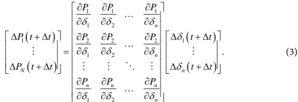
∂ ∂ ∂  _…  _{∂ ∂ ∂}      ∆ + ∆ ∆ + ∆   ∂ ∂ ∂   …     _{∂ ∂ ∂}   =         ∆ + ∆  ∆ + ∆    _{ }  ∂ ∂ ∂  _…  _{∂ ∂ ∂}          (3)

In [1], it was shown that a discreet derivative approach was sufficient to as-certain the majority of information available through the buses with PMUs and generate the diagonal terms. This led to an eigenvalue matrix to approximate the Jacobian’s eigenvalues presented in Equation (4) for the decoupled real power portion.

(

)

(

)

( )

( )

( )

( )

(

)

(

)

0 0 .

0 0

n n n

n

P t t

P t t t t

P t t P t t t

t δ δ δ δ ∆   _∆  ∆ + ∆ ∆ + ∆   _{ }   _{= }    _{ }  ∆ + ∆   ∆ ∆ + ∆       _∆   

   (4)

The error associated with the DDJEA method was calculated using Equation (5) and presented in Table 1.

100. actual predicted err actual P P P P −

= ∗ (5)

(

)

( )

(

)

i predicted i acutal i

P t+ ∆t =P t + ∆P t+ ∆t (6)

(

)

(

)

i actual i itotal V i I i

P t+ ∆t = ∗V ∗I ∗ δ −δ (7)

1i

V is the corresponding average positive sequence voltage magnitude at a bus

(i). I1itotal is the average net positive sequence current flowing through bus (i).

The corresponding phase angle for V1i is δV i1, and δI i1 is the phase angle for

1itotal

I .

The predicted change calculated via the DDJEA matrix of the previous itera-tion was compared to the actual value measured during the next iteraitera-tion. As-suming that the Jacobian should not change dramatically, unless under a serious system event, the assumption was made that the 0.0333 second interval would be sufficiently small enough to apply the Jacobian of the last cycle and compare the

Table 1. DDJEA accuracy for real power estimation.

Calculation source

Percent error of real power (Perr) for measurements

Mean percent error (Perr) Median percent error (Perr)

IEEE 14 bus

simulation 0.054% 9.51 × 10−6%

Open PDC

changes in the eigenvalue. This theory was shown to hold in [1]. The proposed expansion should ultimately take the form of Equation (8). The expansion of the DDJEA matrix, abbreviated EDDJA for further reference, increases the number of critical terms in the matrix through statistical analysis and least squares analy-sis. This portion of the expansion is better suited to an offline analyanaly-sis. Although the process is quick, it would not be applicable for a real-time calculation since a large running window of data is needed first. Once the model is built, it is appli-cable for constant use in future matrices.

(

)

(

)

( )

( )

_{( )}

( )

( )

_{( )}

( )

( )

_{( )}

( )

( )

_{( )}

( )

( )

_{( )}

( )

( )

_{( )}

( )

( )

_{( )}

( )

( )

_{( )}

( )

( )

_{( )}

(

)

(

)

1 1 1

11 12 1

1 2

2 2 1 1

21 22 2

1 2 1

1 2 1 2 . n n n n n

n n n

n n nn

n

P t t

P t t

P t P t P t

t t t

t t t

P t P t P t t t

t t t

t t t

t t

P t P t P t

t t t

t t t

α α α

δ δ δ

δ

α α α

δ δ δ

δ

α α α

δ δ δ

∆ + ∆    _{ =}   _{∆ + ∆}     ∆ ∆ ∆   _{∆ ∆ ∆}     _{∆ ∆ ∆} _{∆ + ∆ }  _{  } ∆ ∆ ∆  _{  }  _{ ∆ + ∆ }      _{∆ ∆ ∆}   …  ∆ ∆ ∆             (8)

In order to determine significant terms, a linear model was built over 4000 real power samples per bus from actual industry PMU data. This results in a [4000 × n] matrix that applies least squares analysis to determine significant terms. The Gaussian distribution of each term is used to evaluate the usefulness of the overall model and significance of each individual term. All non-significant terms become 0 while the significant terms will hold a value. The significant terms will not ultimately hold the value assigned by the linear model, since the linear model produces constant terms without a time-varying property. Due to the chaos of this sample, the linear model is ineffective in managing the residual errors, causing a poor value over a long sampling period for the coefficient of determination, R2_{. However, this will be resolved in the following derivations}

since the linear model assumes a constant value per term instead of the time va-rying weights desired in Equation (8). For a single bus at time t + Δt, the equa-tion for power would be:

(

)

( )

( )

_{( )}

(

)

1

n

i

i ij j

j j

P t

P t t t t t

t α δ δ = ∆ ∆ + ∆ = ∗ ∗ ∆ + ∆ ∆

∑

The term αij

( )

in-significant will have an αij

( )

(

)

(

)

n

i ij

j

x t t x t t

=

+ ∆ =

∑

(

)

( )

_{( )}

(

)

1 1

1

i

P t

x t t t t

t δ

δ ∆

∆ ∆

∆

+ ∆ = ∗ + (11)

(

)

( )

_{( )}

(

)

11 1

1

P t

x t t t t

t δ

δ ∆

∆ ∆

∆

+ ∆ = ∗ + ₍₁₂₎

Each independent variable takes the form of a column vector. ∆P1actual is a

column vector storing the actual change in power at each time interval. The column vector X11 is used to show the predicted value of the change in power at

bus (1) by assuming all change is due to the angle of bus (1). It is important to note that for (n) PMU buses, there will be (n) X column vectors for every

i actual

P

∆ column vector. There are a total of (n) ∆Pi actual column vectors that are

used to individually define the outcome for the linear model at each bus (i).

(

)

(

)

(

)

(

)

4000

x t t

x t t

X

x t t

 + ∆   _{+ ∆}    × =     + ∆    

 (13)

(

)

(

)

(

)

(

)

4000 actual actual actual

actual

P t t

P t t

P

P t t

 +   ₊    ∆ _{× =  }   +     ∆ ∆ ∆ ∆ ∆ ∆

 (14)

Each bus has (n) X column vectors to be statistically evaluated. The linear model uses least squares to fit a weight to each variable for the overall sample period. If an X value is substituted, the weights will return the overall change in bus power. The final linear model for bus 1 is shown in Equation (15) and ex-panded generically in Equation (16). R code was used to carry out this analysis.

( )

( )

1 1 1

1

n

j j

j

P T

β

=

∆ =

_∑

This equation assumes that the time T is at the exact instance desired. β1j is

the weight given to the term correlating the change in real power at bus (1) with respect to bus (j). Unlike equation (6), the weight of each term is not time vary-ing; it is set to a constant by the least squares optimization.

( )

( )

( )

( )

( )

1 11 11 12 12 13 13 1n 1n

P T β X T β X T β X T β X T

∆ = ∗ + ∗ + ∗ ∗∗ ∗ (16)

The pvalue of the overall model is then determined to evaluate the significance

of the model. All values for T =t to T = +t 4000∆t are considered. A p_value

less than 0.05 generally will suffice to show that the model is significant, but this term can be set to a different value. This would equivalently mean that the model has a 95% chance of being significant. For this particular application, the level of significance was much lower. The overall linear model for the industry system yielded a pvalue less than 10−12, meaning that the null hypothesis would be

term was tested, setting 0.0001 as the level of significance (a 99.99% threshold that each term considered is significant), in order to determine a single term’s effectiveness at predicting the real power change. Only those with lower pvalue

calculations would remain, meaning that individually those terms were adequate to predict the change in real power. This reduction for non-significant terms is shown in Equation (17).

1 1

For 0.0001, 0

i i

p_β > β = (17)

All nonzero terms are then placed back in the matrix, and all insignificant terms become zero, showing that there is no connectivity in the reduced model. All off-diagonal terms that are non-zero imply a strong correlation between the buses, and in the context of the power flow Jacobian, some generalization of connectivity. However, the weights used for the overall model are not adequate when looking at longer time periods. In order to get a running window, an overdetermined equation is formed in order to solve for the weights of all non-zero terms in real-time. The mathematical concept is demonstrated with a 4 bus model for simplicity. In this model, there is connectivity between buses 1 and 2, as well as 3 and 4.

(

)

(

)

(

)

(

)

( )

( )

_{( )}

( )

( )

_{( )}

( )

( )

_{( )}

( )

( )

_{( )}

( )

( )

_{( )}

( )

( )

_{( )}

( )

( )

_{( )}

( )

( )

_{( )}

(

)

(

)

(

)

2 2 1

21 22

1 2 2

3 3 3 33 34 4 3 4 4 4 43 3 4 2 3 4 0 0 0 0 0 0

0 0 _nn

P t t

P t t

P t t

P t t

P t P t

t t

t t

P t P t t t

t t

t t t t

t t

P t P t

t t

t

t t

P t P t

t t t t α α δ δ δ α α

δ δ δ

δ

α α _δ

δ δ α α δ δ ∆ ∆ ∆ ∆ ∆ ∆ ∆ ∆ ∆ ∆ ∆ ∆ ∆ ∆ ∆ ∆ ∆ ∆ ∆ ∆ ∆ ∆ ∆ ∆ ∆ ∆ ∆ ∆ ∆ ∆ ∆  +   ₊   _{ =}  ₊    +             ₊     +   ₊              

(

)

         +  ∆  (18) In order to calculate the variable terms in a single row, the equation can be set up ignoring all zero terms. If the number of non-zero terms is M, in this case M

= 2 for each row, then a running window of M + 1 equations is necessary to ap-ply least squares. The back calculation for α11 and α12 are as follows in Equa-tions (19 - 22).

(

)

(

)

( )

(

)

(

)

(

)

(

)

( )

( )

( )

( )

1 11 12

11

1 11 12

12

1 11 12

2 2 2

P t t x t t x t t

t

P t t x t t x t t

t

P t x t x t

α α − − −        ₋  _{= − −}                 ∆ ∆ ∆  ∆ ∆ ∆ ∆ ∆ ∆ (19)

(

)

(

)

(

)

(

)

( )

( )

x t t x t t

A x t t x t t

x t x t

− −     =_ − − _    ∆  ∆ ∆

(

)

(

)

( )

1

1

1

2

P t t

B P t t

P t

∆ ∆

∆ ∆

−

 

 

=_ −  ∆ 

 

(21)

( )

( )

( )

1

11 T T

12

t

A A A B

t α α

−

 

= ∗ ∗

 

  (22) In an extensive system, it is worthwhile to run a sufficiently large sample size offline to attain a generalized system topology between the PMU buses. Then that topology can be used for online application. Before the running window has been met, M + 1 full readings, the original DDJEA method is implemented, us-ing the eigenvalue approximation approach to estimate critical system informa-tion. Once the necessary window has been met, the EDDJA method is applied to calculate weights for each component. Unlike the linear model constants, these weights change with time. Each weight is calculated over a very small time pe-riod, since the Jacobian should not change significantly. These weights allow the impact and importance of each term to change over time, especially as system conditions change or during an event such as a fault. The R2 _{value of the}

indi-vidual models tend to be above 0.9995 with almost all error reduced from each windowed model, effectively solving the main concern of using a universal vari-able to calculate the weight of each term. The general connectivity is solved over one long running window, but the individual terms can take different magni-tudes and sign over days.

Equation (5) is applied to the outcome of using the DDJEA method from Eq-uation (4) in order to estimate the power at the t+ ∆t time step for Table 1.

Equation (5) is also used to calculate the percent error when using the expanded discreet Jacobian approximation, EDDJA, in Equation (8) to ascertain the effec-tiveness of the EDDJA method. The percent error of the predicted real power and actual real power is improved by the EDDJA method for both simulated and real industry case, with the DDJEA and EDDJA methods displayed in Table 1

and Table 2. The industry system had the outputs recorded for 147.5 seconds, 4225 individual time steps, same as in [1] for comparison of the methods. The IEEE 14 bus system was simulated with a three phase fault which cleared via line removal after 0.1 seconds. Table 3 shows the magnitude of error that was re-duced by using EDDJA over DDJEA to approximate the next real power state.

By increasing the number of important terms and giving those terms weights based on a running least square windowing method, EDDJA reduces the percent error by orders of magnitude shown in Table 3.

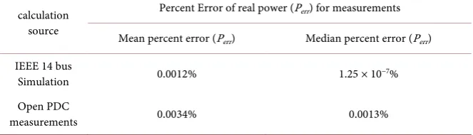
Table 2. EDDJA accuracy for real power estimation.

calculation source

Percent Error of real power (Perr) for measurements

Mean percent error (Perr) Median percent error (Perr)

IEEE 14 bus

Simulation 0.0012% 1.25 × 10−7%

Open PDC

measurements 0.0034% 0.0013%

Table 3. EDDJA error reduction compared to DDJEA.

Calculation source

Percent error reduction of real power (Perr) measurements

Mean percent error magnitude

reduction Median percent error magnitude reduction

IEEE 14 bus

simulation 45x 76x

Open PDC

measurements 58x 77x

linearity and reduced complexity of a simulated system. EDDJA produced an approximate Jacobian than adequately fulfilled the function of the actual de-coupled power flow Jacobian. It also out-performed the DDJEA method pre-viously introduced.

2.2. Expanding DDJEA to EDDJA for Δ

Q

The derivation for the decoupled reactive power portion of the Jacobian follows the same pattern as the real power portion of the decoupled Jacobian. The fol-lowing equations present the derivations for ΔQi, the change in reactive power at

bus (i). All mathematical notation follows the same notation as the equations in section 2.1.

1 .

N i j

i j i

j j V Q Q V V V = ∂ _∗ ∆ ∂

∆ =

∑

(

)

sin .

i i

i ij i j ij j k

j

V Q

V Y V V

V

θ

δ

δ

∂

= − + −

∂

(24)

(

)

( )

(

)

i predicted i i

Q t ∆t Q t ∆Q t t

∴ + = + + ∆

(25)

(

)

(

)

i actual i itotal V i I i

Q t+∆t = ∗V ∗I ∗ δ −δ

(26)

(

)

(

)

( )

( )

( )

( )

( )

( )

(

)

(

)

(

)

(

)

0 0 .

0 0

n n n

n

n n

Q t V t t

V t

V t V t t

Q t t

Q t t Q t V t t

V t

V t V t t

100. actual predicted err actual Q Q Q Q − = ∗ (28)

(

)

(

)

(

)

(

)

(

)

(

)

1 1 1

1 1 1

1

1 2

1

1 2 2 2

2 2 2

1 2 1 2 . n n N n

n n n n

n n n

n

Q Q Q

V V V

V t t

V V V

V t t

Q t t Q P P

V V V

V V

Q t t V t t

P P P V t t

V V V

δ

δ δ δ

∂ ∂ ∂  _{∗ ∗ … ∗}  _{∂ ∂ ∂} _{ + }  _{  } +   +   ∂ ∂ ∂ _{ } ∗ ∗ … ∗    _{= ∂ ∂ ∂  }     _{ }    ₊  ₊ ∆ ∆ ∆ ∆ ∆ ∆ ∆ ∆ ∆ ∆    _{   }  ∂ ∂ ∂ +  _{∗ ∗ … ∗   } _{∂ ∂ ∂}          (29)

(

)

(

)

( )

_{( )}

( )

( )

( )

( )

_{( )}

( )

( )

( )

_{( )}

( )

( )

_{( )}

( )

( )

( )

_{( )}

( )

( )

( )

_{( )}

( )

( )

( )

_{( )}

( )

( )

( )

_{( )}

( )

( )

( )

( )

_{( )}

( )

1 1 1

11 1 12 1 1 1

1 2

2 2 2

1

21 2 22 2 2 2

1 2

1 2

1 2

n n n

n n n n n n

n n n nn n

n

Q t Q t Q t

t V t t V t t V t

V t V t V t

Q t Q t Q t

Q t t

t V t t V t t V t

V t V t V t

Q t t

Q t Q t Q t

t V t t V t t V t

V t V t V t

α α α

α α α

α α α

∆ ∆ ∆ ∆ ∆ ∆ ∆ ∆ ∆ ∆ ∆ ∆ ∆   ∗ ∗ ∗       +  _{  } ∗ ∗ ∗  _{ =  }  _{  }  +    ∆ ∆ ∆ ∆ ∆ ∆ ∆ ∆      ∗ ∗ ∗   ∆          

(

)

(

)

(

)

(

)

V t t

V t t

V t t

V t t

+    ₊       ∆ ∆ ∆  +    ₊     ∆ ∆ ∆

 (30)

(

)

_{( )}

( )

( )

₍

(

₎

)

11 1

1 1

Q

Q t V t t

x t t V t

V t V t t

∆ ∆ + ∆

+ ∆ = ∗ ∗

∆ + ∆ (31)

( )

( )

1 1 1

1

n

j iQ

j

Q T

β

=

∆ =

∑

1 1

For 0.0001, 0

i i

pβ > β = (33) The same IEEE 14 bus system data and industry PMU data were used to test the reactive power case. Table 4 displays the accuracy of the DDJEA method, while Table 5 shows the accuracy in predicting the next reactive power state when using the EDDJA algorithm. Table 6 demonstrates the magnitude of the error reduction by using EDDJA compared to DDJEA.

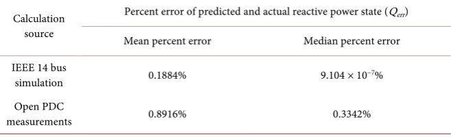
In the IEEE 14 bus simulation, the error when predicting the reactive power state was reduced almost entirely. For the industry measurements, the errors were reduced significantly, but not by the same margin. Generators are set to supply consistent real power output. The reactive power fluctuates to maintain the real power output. In the simulated system, there was far less variation, even with simulated system events. In the real system, the reactive power fluctuated wildly, something to expect with significantly more loads and 3000 more buses

Table 4. DDJEA accuracy for reactive power estimation.

Calculation source

Percent error of predicted and actual reactive power state (Qerr)

Mean percent error Median percent error

IEEE 14 bus

simulation 0.1884% 9.104 × 10−7%

Open PDC

Table 5. EDDJA accuracy for reactive power estimation.

Calculation source

Percent error of predicted and actual reactive power state (Qerr)

Mean percent error Median percent error

IEEE 14 bus

simulation 3.91 × 10−5% 1.137 × 10−11%

Open PDC

measurements 0.1435% 0.1027%

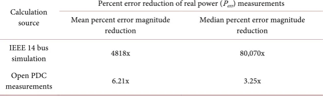
Table 6. EDDJA error reduction compared to DDJEA for reacrive power.

Calculation source

Percent error reduction of real power (Perr) measurements

Mean percent error magnitude

reduction Median percent error magnitude reduction

IEEE 14 bus

simulation 4818x 80,070x

Open PDC

measurements 6.21x 3.25x

in the overall system. The EDDJA method was able to reduce a significant amount of error from the system while adding a negligible amount to the overall computation time, as much as 40%., converging before the next iteration is read. The EDDJA method generates a reduced matrix that accurately functions as a Jacobian approximation. The novel method also proves itself an improvement in comparison to the DDJEA method for approximating the reactive portion of the decoupled power flow Jacobian.

3. Implementing EDDJA for Situational Awareness and

Stability Analysis

and magnitude variation.

EDDJA requires eigenvalue calculation and Singular Value Decomposition is used to quantify bus eigenvalues into different zones during an event or unstable oscillation. Knowing which buses and parameters are most effected during the onset of unstable conditions can aid system operators in isolating and fixing the issue. The eigenvalue for EDDJA is similarly utilized in Equations (37 - 39). “AI” denotes the acceleration indicator. These equations below are derived for the real power portion of DDJEA and EDDJA. The reactive power decoupled por-tions are derived similarly.

( )

( )

( )

( )

( )

(

(

)

)

(

(

)

)

(

(

)

)

2 . 2

DDJEA

i i i i i

i i i i i

AI t

P t P t P t t P t t P t t

t t t t t t t t

δ δ δ δ δ

=

   −   − − 

= − − −

     

  

∆

  

− − −

  

∆ ∆ ∆ ∆ ∆ ∆ ∆

∆

∆ ∆ ∆ ∆ _{  ∆} ∆ ∆ _{∆ }

(34)

( )

(

)

0 bus DDJEA is accelerating.

DDJEA DDJEA

AI t − AI t− ∆ > →t (35)

( )

( )

(

(

)

)

i i

i i

P t P t t

t t t

δ

δ

 ∆ ∆ − ∆ 

− > →

 

_{∆ ∆ − ∆} 

  (36)

( )

(

)

( )

(

( )

)

(

)

(

)

(

(

( )

)

(

)

(

( )

)

(

)

)

( )

(

)

0 bus EDDJA is accelerating.

EDDJA EDDJA

AI t − AI t− ∆ > →t (38)

( )

(

)

( )

(

( )

)

(

)

(

)

0 bus EDDJA is increasing.

eig Bus i t − eig Bus i t− ∆t > →

(39) Since singularities are the mathematical indication of instability in terms of DDJEA and EDDJA elements, acceleration toward zero and infinity should al-ways be flagged. By analyzing EDDJA, both static and dynamic stability margins can be assessed. Furthermore, a continually increasing eigenvalue outside of equilibrium can be flagged so that slow inter-area oscillations are not missed. Immediately after system events, acceleration back toward the equilibrium point is noted and system parameters are updated should a solution not be necessary. In [1], the DDJEA algorithm was applied for situational awareness and flagging critically unstable parameters. Singular Value Decomposition is applied in this model to achieve an index for eigenvalues, similar to [2] [3] [4] [5] [6]. Figure 1

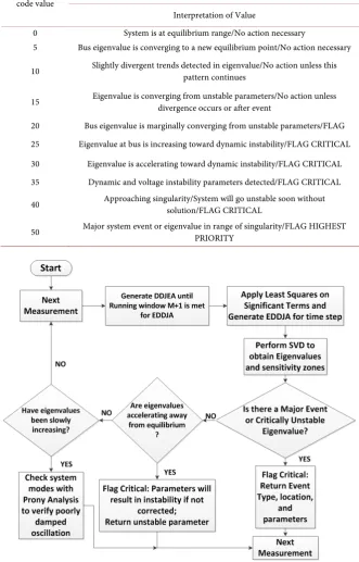
shows the general algorithm that EDDJA implements to enhance situational awareness. Table 7 decodes the output of the graphs for both DDJEA and EDDJA in Figure 2 and Figure 3 respectively. These methods are compared to the output of Prony Analysis in Figure 4 to showcase EDDJA’s immediate de-tection of an unstable system mode in comparison with a well-known method.

Table 7. DDJEA and EDDJA analysis code value interpretation.

code value Figure 2/Figure 3 decode table

Interpretation of Value

0 System is at equilibrium range/No action necessary

5 Bus eigenvalue is converging to a new equilibrium point/No action necessary

10 Slightly divergent trends detected in eigenvalue/No action unless this _{pattern continues}

15 Eigenvalue is converging from unstable parameters/No action unless _{divergence occurs or after event}

20 Bus eigenvalue is marginally converging from unstable parameters/FLAG

25 Eigenvalue at bus is increasing toward dynamic instability/FLAG CRITICAL

30 Eigenvalue is accelerating toward dynamic instability/FLAG CRITICAL

35 Dynamic and voltage instability parameters detected/FLAG CRITICAL

40 Approaching singularity/System will go unstable soon without _{solution/FLAG CRITICAL}

50 Major system event or eigenvalue in range of singularity/FLAG HIGHEST _PRIORITY

Figure 1. EDDJA analysis for applied situational awareness.

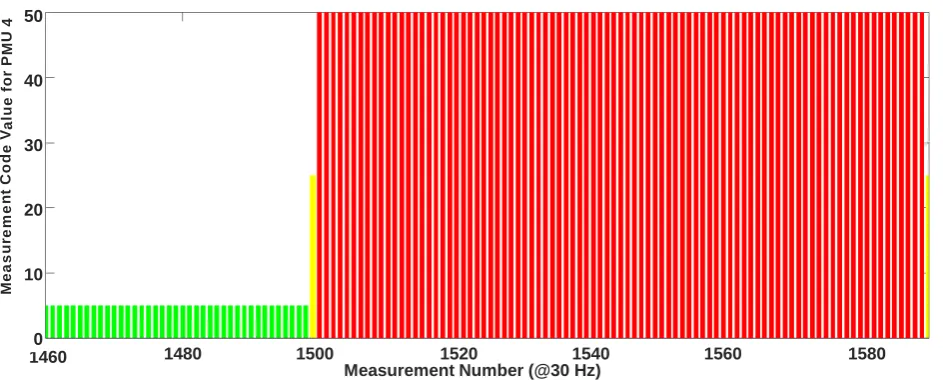
Figure 2. DDJEA analysis outputfor unstable case.

in Figure 3. Figure 4 demonstrates that the weighted off-diagonal terms are consistently unstable when their time-varying weights are applied. The initial event detection of DDJEA and EDDJA are comparable, but the eigenvalues of the EDDJA matrix show more consistency when identifying both dynamic and static instability due to the additional weighted terms in both the real and reac-tive power decoupled Jacobian matrix approximations. This implementation of SVD and eigenvalue analysis correlates with [2] [3] [4] [5] [6]. Since the weak point and parameters could have been relayed, this unstable condition could have been prevented by having system operators manually remove the affected line without voltage collapse.

The output of these methods can be compared with event detection using Prony analysis for comparison of effectiveness and response time. It is viable to note that Prony Analysis does not converge in real-time for all buses and there-fore is better used to monitor inter-area oscillations, and modes approaching marginally stable conditions [7] [8]. Equations (40) and (41) show the general output of Prony Analysis.

( )

(

)

1

e j cos 2π .

M

t

j j j

j

F t

α

φ

=

=

∑

( )

1

e ie .i

M

j t i i

F t β ±φ λ

=

=

∑

The signal is decomposed into a series of weighted, damped sinusoids. The eigenvalues are put into state-space form, terms with weights near zero are re-moved, and the fundamental mode and corresponding eigenvalues are returned. The signal under analysis is the real power at each PMU bus. The power through the bus is analyzed for poorly damped or unstable dominant modes. Prony Analysis was applied to the same unstable data set as DDJEA and EDDJA. The interpreted output is shown in Figure 4 with Table 8 detailing the individual output levels.

Measurement Number (@30 Hz)

1460 1480 1500 1520 1540 1560 1580

Measurement Code Value for PMU 4

Figure 3. EDDJA analysis outputfor unstable case.

Figure 4. Prony analysis output for unstable case.

Table 8. Prony analysis code value interpretation.

Code value Figure 4 decode table

Interpretation of value

0 Damping ratio is above 5% and frequency is not shifting significantly

1 System mode and eigenvalue are shifting significantly

2 Damping ratio under 5%/Flag oscillation

3 Damping ratio is under 1% and eigenvalue’s real part is reaching 0/Flag criti-_cal

4 A dominant system mode has a positive real part [Unstable _{condition]/FLAG HIGHEST PRIORITY}

Prony analysis detects a significant shift in the dominant mode, but the first unstable eigenvalue is not read for 10 cycles. Prony analysis registers a consis-tently unstable dominant eigenvalue at the same PMU however after several

Measurement Number (@30 Hz)

1460 1480 1500 1520 1540 1560 1580

50

40

30

20

10

0

M

e

a

s

u

re

m

e

n

t

C

o

de Va

lu

e

fo

r

PM

U

4

Sample Number (@30Hz)

1480 1490 1500 1510 1520 1530 1540 1550 1560

Code Value

cycles have passed, verifying that the EDDJA method more accurately reflects the nature of the bus eigenvalues than the DDJEA method. In terms of situa-tional awareness, Prony analysis is well suited to be run alongside the EDDJA method to help identify and verify unstable power oscillations early on for buses that have marginally divergent EDDJA indications.

4. 1-D Biorthogonal Wavelet Event Detection and

Identification

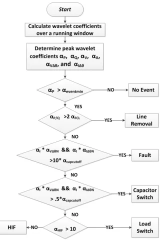
The 1-D discreet biorthogonal wavelet was selected for processing the individual signals. The signals were analyzed with a variety of wavelets including Haar, Meyer, and Symlet wavelets. The Matlab “bior3.5” wavelet function was ulti-mately used to generate the wavelet coefficients. These coefficients were ana-lyzed across several different cases containing a fault, capacitor switch, HIF, load switch, and line removal. Peak wavelet coefficients for the real power, reactive power, phase voltage magnitude, phase current magnitude, discreet derivative of the voltage phase angle, and discreet derivative of the current phase angle. Equa-tion (42) shows the general format from which the wavelet coefficients are ulti-mately derived.

(

)

( )

( )

W_ψ a d =

∫

( )

Figure 5. Biorthogonal wavelet event identification.

→ The peak wavelet coefficient associated with the real power signal; → The peak wavelet coefficient associated with the reactive power signal; → The peak wavelet coefficient associated with the voltage magnitude signal;

→ The peak wavelet coefficient associated with the current magnitude signal;

→ The peak wavelet coefficient associated with the discreet derivative of current phase angle;

eventmin

α → The real power wavelet coefficient used as a cut off many orders above system noise;

capcutoff

α → Lower wavelet bound for typical system capacitors in regards to

; P

α

/

P P Q

Q

α α

α

= (43)

/

P Q

α → Gives a margin to easily detect line removals; All other events fall near 1 or under;

FCL

α →Calculated by creating a gaussian distribution over a range of data: → Then the value is calculated for having a 1% level of significance, meaning that;

→ 1 out of every 100 rejections will be false. When the number is doubled, the odds converge;

→ Toward zero.

0.001

V

V N

α

α ∆Θ

∆Θ = → This is just an applied weight for certain calculations (44).

0.001

I

I N

α

α ∆Θ

∆Θ = (45)

The low impedance fault stands out statistically in wavelet transforms. The HIF can be hard to determine, but it affects the discreet derivative of the voltage angle significantly more in most cases than a load switch. A load switch dwarfs the impact that an HIF appears to have on the system from time domain sam-ples, but by highlighting the one area that HIF has a greater magnitude, a term can be generated that drives a load switch toward a higher value and an HIF to-ward zero. This guarantees that even a small load switch cannot drive toto-ward zero due to its effect on the circuit. This term is called αHIF.

V HIF

I

α

α

α

∆Θ

∆Θ

= ₍₄₆₎

Figure 5 shows the general algorithm for applying wavelet transforms for event detection and identification.

In the case of all tested events, this model was able to adequately identify the event type. Statistical analysis is a powerful addition to this model when selected the cutoff values. Analyzing the mean and standard deviation of different event types can help distinguish event characteristics. The detection of HIF characte-ristics through PMU data was a fantastic breakthrough, since a lot of publica-tions use transient data for detection. PMU data can cover a much larger time segment in fewer points, but there is also less resolution than samples with 1,000,000 Hz sampling rates. This is an advantage since smaller window lengths are required to enclose the event and its residual effects to the system.

5. Conclusion

where system connectivity is unavailable, making it an excellent model-free analysis method. The conditions and options to include both Prony analysis and wavelet decomposition were expressed. EDDJA yields incredibly accurate eigen-value information, leading to more accurate identification of unstable parame-ters and increased system visibility with respect to which buses are influencing an unstable parameter. Prony analysis verified the estimate of unstable eigenva-lues by EDDJA. Prony analysis and wavelet decomposition are both ideal tools to use along with this method to give system operators verification and time to solve oscillatory power flow and event types. In the case of events, wavelet analy-sis can be used to double check the cause of changes in the Jacobian. The wavelet transform was able to detect and identify all system events including the HIF from PMU data, which is significant since the majority of publications apply wavelet transforms to transient data sets. Future research will most likely incor-porate Machine Learning to wavelet outputs to train a more flexible algorithm that can immediately analyze data without further offline analysis.

Acknowledgements

The authors would like to thank the members of Clemson University Electric Power Research Association (CUEPRA) for their financial support and provid-ing PMU data.

References

[1] Kantra, S.D. and Makram, E.B. (2016) Development of the Decoupled Discrete- Time Jacobian Eigenvalue Approximation for Situational Awareness Utilizing open PDC. Journal of Power and Energy Engineering, 4, 21-35.

https://doi.org/10.4236/jpee.2016.49003

[2] Sauer, P.W. and Pai, M.A. (1990) Power System Steady-State Stability and the Load- Flow Jacobian. IEEE Transactions on Power Systems, 5, 1374-1383.

http://ieeexplore.ieee.org/stamp/stamp.jsp?tp=&arnumber=99389 https://doi.org/10.1109/59.99389

[3] Bompard, E., Carpaneto, E., Chicco, G. and Napoli, R. (1996) A Dynamic Interpre-tation of the Load-Flow Jacobian Singularity for Voltage Stability Analysis. Interna-tional Journal of Electrical Power & Energy Systems, 18, 385-395.

http://ac.els-cdn.com/0142061595000828/1-s2.0-0142061595000828-main.pdf?_tid= 88f8aee4-55d5-11e6-9b87-00000aacb361&acdnat=1469828809_a3d7830991205892b c2111fd63d57c2d

https://doi.org/10.1016/0142-0615(95)00082-8

[4] Lof, P.-A., Smed, T., Andersson, G. and Hill, D.J. (1992) Fast Calculation of a Vol-tage Stability Index. IEEE Transactions on Power Systems, 7, 54-64.

http://ieeexplore.ieee.org/stamp/stamp.jsp?tp=&arnumber=141687 https://doi.org/10.1109/59.141687

[5] Stott, B. and Alsac, O. (1974) Fast Decoupled Load Flow. IEEE Transactions on Power Apparatus and Systems, PAS-93, 859-869.

http://ieeexplore.ieee.org/stamp/stamp.jsp?tp=&arnumber=4075431 https://doi.org/10.1109/TPAS.1974.293985

http://ieeexplore.ieee.org/stamp/stamp.jsp?tp=&arnumber=193851 https://doi.org/10.1109/59.193851

[7] Guoping, L., Ning, J., Tashman, Z., Venkatasubramanian, M. and Trachian, P. (2012) Oscillation Monitoring System Using Synchrophasors. 2012 IEEE Power and Energy Society General Meeting, San Diego, CA, 22-26 July 2012, 1-8.

http://ieeexplore.ieee.org/stamp/stamp.jsp?tp=&arnumber=6345444 https://doi.org/10.1109/PESGM.2012.6345444

[8] Guoping, L. and Venkatasubramanian, M. (2008) Oscillation Monitoring from Am- bient PMU Measurements by Frequency Domain Decomposition.2008 IEEE Inter-national Symposium on Circuits and Systems, Seattle, WA, 18-21 May 2008, 2821- 2824. http://ieeexplore.ieee.org/xpl/articleDetails.jsp?arnumber=4542044

https://doi.org/10.1109/iscas.2008.4542044

[9] Bruelmann, H., Grebe, E. and Losing, M. (2000) Analysis and Damping of Inter- Area Oscillations in the UCTE/CENTRAL Power System.

http://citeseerx.ist.psu.edu/viewdoc/download;jsessionid=4C196EE579817D7A450E AA3A662DA104?doi=10.1.1.124.7846&rep=rep1&type=pdf

[10] Ning, Z., Huang, Z., Tuffner, S., Pierre, J. and Jin, S. (2010) Automatic Implementa-tion of Prony Analysis for Electromechanical Mode IdentificaImplementa-tion from Phasor Measurements. 2010 IEEE Power and Energy Society General Meeting, Minneapo-lis, MN, 25-29 July 2010, 1-8.https://doi.org/10.1109/PES.2010.5590169

http://ieeexplore.ieee.org/xpls/abs_all.jsp?arnumber=5590169&tag=1

[11] Guoping, L., Quintero, J. and Venkatasubramanium, V.M. (2007) Oscillation Mon-itoring System Based on Wide Area Synchrophasors in Power Systems. 2007 iREP Symposium on Bulk Power System Dynamics and Control, VII. Revitalizing Opera-tional Reliability, Charleston, SC, 19-24 August 2007, 1-13.

http://ieeexplore.ieee.org/stamp/stamp.jsp?arnumber=4410548

[12] Wai, D.C.T. and Xia, Y. (1998) A Novel Technique for High Impedance Fault Iden-tification. IEEE Transactions on Power Delivery, 13, 738-744.

http://ieeexplore.ieee.org/stamp/stamp.jsp?arnumber=686968 https://doi.org/10.1109/61.686968

[13] Girgis, A., Chang, W. and Makram, E.B. (1990) Analysis of High-Impedance Fault Generated Signals Using a Kalman Filtering Approach. IEEE Transactions on Pow-er DelivPow-ery, 5, 1714-1724. https://doi.org/10.1109/61.103666

http://ieeexplore.ieee.org/stamp/stamp.jsp?arnumber=103666

[14] Huang, S.-J. and Hsieh, C.-T. (1999) High Impedance Fault Detection Utilizing Morlet Wavelet Transform Approach. IEEE Transactions on Power Delivery, 14, 1401-1410. http://ieeexplore.ieee.org/stamp/stamp.jsp?arnumber=796234

https://doi.org/10.1109/61.796234

[15] Lai, T.M., et al. (2005) High-Impedance Fault Detection Using Discrete Wavelet Transform and Frequency Range and RMS Conversion. IEEE Transactions on Power Delivery, 20, 397-407.https://doi.org/10.1109/TPWRD.2004.837836

http://ieeexplore.ieee.org/stamp/stamp.jsp?arnumber=1375120

[16] Sedighi, A.-R., et al. (2005) High Impedance Fault Detection Based on Wavelet Transform and Statistical Pattern Recognition. IEEE Transactions on Power Deli-very, 20, 2414-2421. http://ieeexplore.ieee.org/stamp/stamp.jsp?arnumber=1514486 https://doi.org/10.1109/tpwrd.2005.852367

Submit or recommend next manuscript to SCIRP and we will provide best service for you:

Accepting pre-submission inquiries through Email, Facebook, LinkedIn, Twitter, etc. A wide selection of journals (inclusive of 9 subjects, more than 200 journals)

Providing 24-hour high-quality service User-friendly online submission system Fair and swift peer-review system

Efficient typesetting and proofreading procedure

Display of the result of downloads and visits, as well as the number of cited articles Maximum dissemination of your research work