Program to Determine the Terrain Roughness Index using Path Profile Data Sampled at Different Moving Window Sizes

Program to Determine the Terrain Roughness Index

using Path Profile Data Sampled at Different Moving

Window Sizes

Simeon Ozuomba

and Computer Engineering University of Uyo Akwa Ibom State Nigeria

Henry Johnson Enyenihi

Engineering, Akwa Ibom State University Mkpat Enin, Akwa Ibom State, Nigeria

Constance Kalu

and Computer Engineering University of Uyo Akwa Ibom State Nigeria

ABSTRACT

In this paper development of a program to determine the terrain roughness index using path profile data sampled at different moving window sizes is presented. Relevant mathematical expressions and algorithm to determine terrain roughness index from elevation data captured at different moving window sizes are presented. The desktop program is written in Visual Basic for Application. The program enables users to sample the elevation data at a given window size and then determine the terrain roughness parameters at any other window size that is multiple of the original sampling window size. Sample 58.5523249 Km study path location that started at a latitude of 5.48717 and longitude of 7.04193 and ended at a latitude of 5.82096 and a longitude of 7.45042 was used to demonstrate the effectiveness of the software. Specifically, Geocontext online elevation profile software is used on the study path to capture N = 512 path profile data at an initial window size of 3.75 seconds which is equivalent to a distance of m. The roughness index is computed at four (4) other sampling window sizes of 30 seconds, 1 minute (60 seconds) , 5 minutes (300 seconds) and 10 minutes (600 seconds). Among other things the program showed the window sizes and their corresponding terrain roughness index along with the elevation profile table and graph for each of the sampling window size. The results show that as the widows size increases the total number of sample data points decreases. Also, the largest terrain roughness index value of 52.89 m is observed with window size of 300 seconds whereas the lowest largest terrain roughness index value of 33.55 m is observed with window size of 600 seconds. The idea presented in this paper is useful for wireless network designer who relies on terrain roughness value for the determination of the multipath fade depth for detailed link design.

Keywords

Multipath, Fading Depth, Terrain Roughness Index, Elevation Profile, Geographic Reference System, Sampling Window

1.

INTRODUCTION

Multipath fading is the losses in signal strength which occurs when signals travel through different paths before they reach the receiver [1, 2,3,4,5,6,7]. The multipath effect will always occur when there is a change in the path of the different components of the signal. As a result of the changes in the signal path, different components of the signal travel through different paths and path lengths before they reach the receiver. In all, at the receiver, the overall signal strength is reduced due to the multipath effect [8,9,10,11].

Notably, the nature of the path elevation profile has been identified as one of the causes of multipath in wireless signal communications systems. Due to the coarse nature of the ground surface signals are reflected at some points as they hit the ground and this ground reflection of signals causes the multipath effect [12,13,14]. Consequently, in a bid to account for the impact of terrain roughness on multipath fading, the International Telecommunication Union (ITU) Recommendation ITU-R P.530-17 incorporated terrain roughness index as part of the parameters for computing multipath fade depth [15].

Basically, the terrain roughness index is the standard deviation of elevation values obtained from the elevation data point captured around the signal path [16,17,18]. However, the approach presented by ITU-R P.530-17 model for computing the terrain roughness index adopted very large distance between elevation data points used in computing the terrain roughness index. As such, researchers in many cases compute terrain roughness index based on elevation data point with a smaller distance between elevation data points [19].

Furthermore, today, there are available online tools for capturing elevation profile data at a different time or distance resolutions. As such, in his paper, the focus is the development of relevant algorithms for a program that will enable users to determine the terrain roughness index of a given area based on the elevation profile data of the area. In the program, it is assumed that the elevation data is captured by an elevation profile data capturing tool that provides information of the distance and elevation of data points along the signal path. It is also assumed that the tool enables the user to select the time interval or distance interval between consecutive elevation data point it will capture and also the interval is the same between all the elevation data points. While the algorithm is presented here , the program is written in Visual Basic for Application (VBA). The requisite mathematical expressions and algorithms used in the program are presented in the succeeding section. The program enables the user to determine the terrain roughness index at higher resolutions that are multiples of the original resolution used to capture the elevation profile data.

2.

METHODOLOGY

2.1

The Theoretical Background On Terrain

Roughness Index

path profile data points considered . Assuming there are N elevation ( data points in the path profile where n = 1,2,…N, then the terrain roughness index ( ) is given as [15];

(1)

Where the average elevation is given as [15];

₍₂₎

In this study, it is assumed that the path profile data is captured at a given constant value moving window size (for instance, one sample every 10 seconds) such that the distance, between sampling point in the given window size, w is equal. The path length, d which is the distance between the starting point (with n = 1) of the profile data sampling to the last point (with n = N) on the data sampling is given as ;

(3)

Where is the distance from data point 1 to data point n, and

. Hence,

(4)

If the elevation at the required distance point p is not available where denotes the distance at point p and denotes the elevation at point p, then interpolation of the two nearest profile points to point d can be used to obtain the elevation,

as follows;

(5)

Where are and are the elevations while and are the distance of the points nearest to the profile point p and .

2.2

The Theoretical Background On The

Sampling Window Sizes

In geographic reference system 1° (that is , 60 minutes or 3600 seconds ) of latitude is equivalent to a distance of 110 Km. Smaller resolution in seconds and minutes can be used whereby 1 second is equivalent to a distance of 30.56 m. In the elevation data capture software tool, the elevation points are captured at a given constant time unit called the sampling window of size, w. It is assumed that the data sampling mechanism moves at a constant speed along the path and captures elevation data every w time units. Since the speed is constant and the sampling window size (time) is also constant, then the distance from one sample point, n to the next sample point n + 1 is constant and it is denoted as , where w represents the sampling window size (time) used. For instance, sampling window size (time) w= 1 second means

= 30.56 m. Other sampling sizes and their corresponding

sampling distance sizes can be obtained from the 1 second window size values. For instance

and . In this paper, the second will be used as the reference time unit to relate the distance among different sampling window sizes.

Now, consider a situation where the software tool is used to capture the elevation data at a window size of seconds which has corresponding sampling distance of and then,

the roughness index parameter is needed at a different sampling size seconds (where ), then the number

(denoted as ) of sample points that will make up one

sample point is given as ;

(6)

Hence,

(7)

For instance, if is 5 seconds such that the

and if the roughness index is required at the sampling rate of then,

and so . In

practice, it is advised that the data capturing windows size be such that the required window sizes for computing roughness index are multiples of the original capturing windows size otherwise the data point will point at the location where there is no elevation data. In such case, interpolation may be used as specified in Equation 5. However, such occasion should be avoided. The total number of data points , when the data is resampled at the window size of from its original

sampling at the window size of is given as ;

(8)

Where means integer part of x.

3.

THE ALGORITHM FOR

DETERMINATION OF THE

TERRAIN ROUGHNESS INDEX

USING PATH PROFILE DATA

SAMPLED AT DIFFERENT MOVING

WINDOW SIZES

The algorithm for the algorithm for determination of the terrain roughness index using path profile data sampled at different moving window sizes are given in following submodules:

Module 1:Read in the N original data points captured by the path profile data capture software toolset at window size

Module 2:Generate data points at another window size , based on the N original data points captured by the path profile data capture software tool

Module 3:Compute the average elevation for the data points at another window size ,

Module 4: Compute the roughness index for the data points at another window size ,

The detailed algorithm is as follows:

Module 1: Read in the N original data points captured by the path profile data capture software toolset at window size

Step 1: INPUT the data capture window size

, , the number of data points , N

Step 2: w =

Step 4: READ the data point distance and the data point elevation

Step 4: NEXT n

Step 5 CALL Module 2

Step 6: END

Module 2:Generate data points at another window size , based on the N original data points captured by the path profile data capture software tool

Step 1: x = 1

Step 2: INPUT the required roughness index

sampling window size ,

Step 3: COMPUTE

Step 4: INITIALISE i = 1 // counter for data points in sampling window size ,

Step 5: FOR n = 1 to N STEP

Step 6: READ the data point distance and the data point elevation

Step 7: =

Step 8: =

Step 9: NEXT n

Step 10: N(x) = i // N(x) is the total number of sampled data points obtained when data is sampled at window size,

Step 11: IF ( is the last window size to

be considered ) THEN

Step 11.1: = x

Step 11.2: CALL Module 3

Step 11.3: ELSE

Step 11.4: x = x + 1

Step 11.5: GOTO Step 2

Step 11.6: ENDIF

Step 12: RETURN

// Compute the roughness index , Sa for the Xn

different window sizes , where x =

1,2,…,Xn

Module 3: Compute the average elevation for the data points at another window size ,

Step 1: x = 1

Step 2: = 0 // Initialise to 0

Step 3: FOR i = 1 to STEP

Step 4: = +

Step 5: NEXT i

Step 6: =

Step 7: IF ( ) THEN

Step 7:1 CALL Module 4

Step 7.2: ELSE

Step 7.3: x = x + 1

Step 7.4: GOTO Step 2

Step 7.5: ENDIF

Step 8: RETURN

Module 4: Compute the roughness index for the data points at another window size ,

Step 1: x = 1

Step 2: = 0 // Initialise sum of squared error, to 0

Step 3: FOR i = 1 to STEP

Step 4: = +

Step 5: NEXT i

Step 6: =

Step 7: IF ( ) THEN

Step 8: GOTO Step 9

Step 8.2: ELSE

Step 8.3: x = x + 1

Step 8.4: GOTO Step 2

Step 8.5: ENDIF

Step 9 RETURN

In the flowchart it is assumed that the window sizes, are multiples of the original sampling window size . In this case no interpolation is required.

A program is written in Visual Basic for Application to automate the computation of the relevant parameters once the required input data are keyed in.

Particularly, the following 4 sets of input data are required for the program ;

i. the number of sampling window sizes to be used

ii. Window sizes , , , …

iii. N , the number of data points for the initial window size

iv. For n = 1 to N input data point distance,

and data point elevation of the initial

window size

i. Sampling Window Size Name, where x = 0,1,2,…

ii. Sampling Window Size in Time Unit (seconds)

iii. Sampling Window Size in Meters

iv. : the number of units of Window Size

that make up 1 Window Size

v. : Total number of sampled data points for Window Size

vi. For n = 1 to output data point distance,

and data point elevation of window size vii. Sumx : Sum of elevations for Window Size

viii. AVGx : Average of elevations for Window Size

ix. SumSqx: Sum of square error of elevations for Window Size

x. Sax : Terrain roughness index for Window Size

4.

NUMERICAL EXAMPLE

The 58.5523249 Km study path location started at a latitude of 5.48717 and a longitude of 7.04193 and ended at a latitude of 5.82096 and a longitude of 7.45042. Geocontext online elevation profile software is used on the study path to capture N = 512 path profile data at an initial window size

of 3.75 seconds which is equivalent to a distance of

m. Meanwhile the roughness index is required at the following four (4) sampling window sizes; 30 seconds, 1 minute (60 seconds) , 5 minutes (300 seconds) and 10 minute s(600 seconds). Accordingly, the program presented in this paper is used to compute the roughness index for the each of the given 4 different sampling window sizes

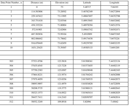
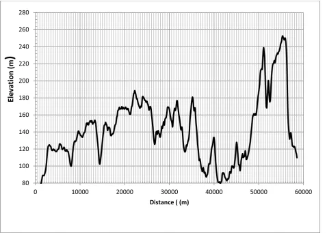
A portion of the originally sampled data using window size , of 3.75 seconds is shown in Table 1 while the elevation profile of the complete path is shown in Figure 1.

Table 1 Portion of the originally sampled data using window size , of 3.75 seconds

Data Point Number , n Distance (m) Elevation (m) Latitude Longitude

1 0 73 5.48717 7.04193

2 114.583806 73.28502 5.48782349 7.04272894

3 229.167612 73.11905 5.48847697 7.04352788

4 343.751418 72.83546 5.48913045 7.04432682

5 458.335224 71.80804 5.48978394 7.04512576

6 572.91903 72.02904 5.49043742 7.04592471

7 687.502836 72.99104 5.4910909 7.04672365

8 802.086642 71.78662 5.49174438 7.0475226

9 916.670449 73.62459 5.49239785 7.04832155

10 1031.25425 73.39307 5.49305133 7.0491205

503 57521.0706 123.5818 5.81508361 7.44322134

504 57635.6545 123.7228 5.81573655 7.44402119

505 57750.2383 123.0307 5.81638948 7.44482103

506 57864.8221 121.9574 5.81704242 7.44562088

507 57979.4059 123.0356 5.81769535 7.44642073

508 58093.9897 121.6979 5.81834828 7.44722058

509 58208.5735 119.3775 5.81900121 7.44802043

510 58323.1573 116.0922 5.81965414 7.44882029

511 58437.7411 114.2163 5.82030707 7.44962014

Figure 1 The elevation profile of the complete path

The results in Table 2 show the output of the window sizes and the corresponding terrain roughness index. The larger the widow size the larger the value of and the smaller is the total number of sample data points . The largest terrain roughness index value of 52.89 m is observed with a window size of 300 seconds whereas the lowest largest terrain roughness index value of 33.55 m is observed with a window size of 600 seconds.

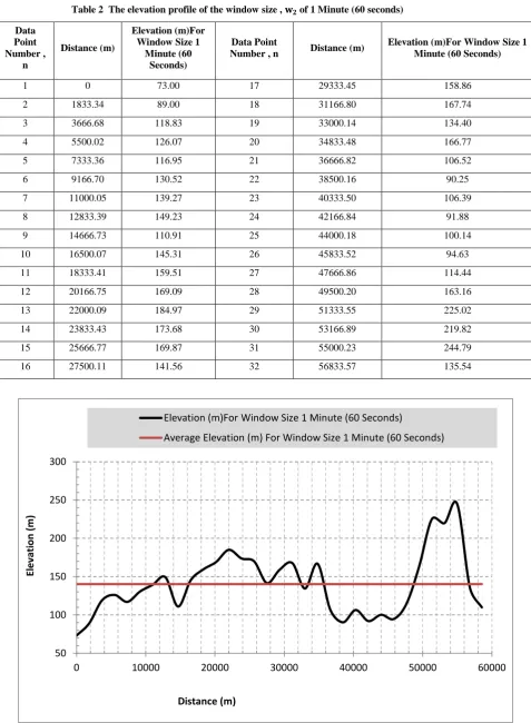
The program also displays the elevation profile table and graph for the various sampling window sizes. Table 2 and Figure 2 show the elevation profile table and graph for the sampling window size , of 1 Minute (60 seconds). A total

of 32 data sampling points are captured with sampling window size of 60 seconds.

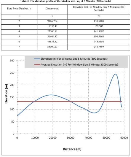
Similarly, Table 23 and Figure 3 show the elevation profile table and graph for the sampling window size , of 5 Minutes (300 seconds). A total of 7 data sampling points are captured with sampling window size of 300 seconds.

.

Table 2 The output of the program showing the window sizes and the corresponding terrain roughness index

Sampling Window Size Name

Sampling Window

Size in Time Unit

(seconds)

Sampling Window

Size in Meters

Total Number Of

Sample Data Points

( )

Sumx AVGx SumSqx Sax

w0 3.75 114.58 512 1 72768.61 142.13 785007.32 39.19

w1 30 916.67 64 8 9220.89 141.86 104735.52 40.45

w2 60 1833.34 32 16 4628.01 140.24 53846.96 41.02

w3 300 9166.70 7 80 1060.41 132.55 19583.69 52.89

w4 600 18333.41 4 160 611.10 122.22 4502.30 33.55

80 100 120 140 160 180 200 220 240 260 280

0 10000 20000 30000 40000 50000 60000

El

e

va

ti

on

(m

)

Table 2 The elevation profile of the window size , of 1 Minute (60 seconds)

Data Point Number ,

n

Distance (m)

Elevation (m)For Window Size 1

Minute (60 Seconds)

Data Point

Number , n Distance (m)

Elevation (m)For Window Size 1 Minute (60 Seconds)

1 0 73.00 17 29333.45 158.86

2 1833.34 89.00 18 31166.80 167.74

3 3666.68 118.83 19 33000.14 134.40

4 5500.02 126.07 20 34833.48 166.77

5 7333.36 116.95 21 36666.82 106.52

6 9166.70 130.52 22 38500.16 90.25

7 11000.05 139.27 23 40333.50 106.39

8 12833.39 149.23 24 42166.84 91.88

9 14666.73 110.91 25 44000.18 100.14

10 16500.07 145.31 26 45833.52 94.63

11 18333.41 159.51 27 47666.86 114.44

12 20166.75 169.09 28 49500.20 163.16

13 22000.09 184.97 29 51333.55 225.02

14 23833.43 173.68 30 53166.89 219.82

15 25666.77 169.87 31 55000.23 244.79

16 27500.11 141.56 32 56833.57 135.54

Figure 2 The elevation profile of the window size , of 1 Minute (60 seconds)

50 100 150 200 250 300

0 10000 20000 30000 40000 50000 60000

El

e

vation

(

m

)

Distance (m)

Elevation (m)For Window Size 1 Minute (60 Seconds)

Table 3 The elevation profile of the window size , of 5 Minutes (300 seconds)

Data Point Number , n Distance (m) Elevation (m) For Window Size 5 Minutes (300 Seconds)

1 0 73

2 9166.704 130.5188

3 18333.41 159.505

4 27500.11 141.5607

5 36666.82 106.5168

6 45833.52 94.63456

7 55000.23 244.7859

Figure 3 The elevation profile of the window size, of 5 Minutes (300 seconds)

5.

CONCLUSION

Mathematical expressions and algorithm along with a program to determine terrain roughness index from elevation data captured at different moving window sizes are presented. The elevation data profile is captured using an online elevation profile data software which captures elevation data at a given regular time or distance interval (window sizes). The program enables users to sample the elevation data at a given window size and then determine the terrain roughness parameters at any given window size that is multiple of the original sampling window size. The program is written in Visual Basic for Application (VBA) and it is a desktop application. Sample path profile is used to demonstrate the

effectiveness of the program to determine the essential terrain roughness parameters for different sampling window sizes.

6.

REFERENCES

[1] Ellis, T., & Weiss, S. (2018, April). Propagation Prediction for Rail Communications in Urbanized Areas. In 2018 Joint Rail Conference (pp. V001T03A006-V001T03A006). American Society of Mechanical Engineers.

[2] Reis, S., Pesch, D., Wenning, B. L., & Kuhn, M. (2018, April). Empirical path loss model for 2.4 GHz IEEE 802.15. 4 wireless networks in compact cars. In Wireless

0 50 100 150 200 250 300

0 10000 20000 30000 40000 50000 60000

El

e

va

ti

on

(m

)

Distance (m)

Elevation (m) For Window Size 5 Minutes (300 Seconds)

Communications and Networking Conference (WCNC), 2018 IEEE (pp. 1-6). IEEE.

[3] Dove, I. (2014). Analysis of radio propagation inside the human body for in-body localization purposes (Master's thesis, University of Twente).

[4] Parasuraman, R., Kershaw, K., & Ferre, M. (2013). Experimental investigation of radio signal propagation in scientific facilities for telerobotic applications. International Journal of Advanced Robotic Systems, 10(10), 364.

[5] Sachdeva, N., & Sharma, D. (2012). Diversity: A fading reduction technique. International Journal of Advanced Research in Computer Science and Software Engineering, ISSN.

[6] Trenggono, P. P. (2011). Statistical modelling of wind effects on signal propagation for wireless sensor networks (Doctoral dissertation, Queensland University of Technology).

[7] Sim, C. Y. D. (2002). The propagation of VHF and UHF radio waves over sea paths (Doctoral dissertation, University of Leicester).

[8] Píšová, P., & Chod, J. (2015). Detection of GNSS signals propagation in urban canyos using 3D city models.

[9] Gibson, J. D. (Ed.). (2012). Mobile communications handbook. CRC press.

[10]Appana, D. K., Kumar, C. A., & Nagappan, N. P. (2009). Channel Estimation in GPRS based Communication System using Bayesian Demodulation.

[11]Miu, A., Tan, G., Balakrishnan, H., & Apostolopoulos, J. (2004, June). Divert: fine-grained path selection for wireless LANs. In Proceedings of the 2nd international conference on Mobile systems, applications, and services (pp. 203-216). ACM.

[12]Ilcev, S. D. (2011). Surface Reflection and Local Environmental Effects in Maritime and other Mobile

Satellite Communications. International Recent Issues about ECDIS, e-Navigation and Safety at Sea: Marine Navigation and Safety of Sea Transportation, 129. [13] Zhao, X. (2002). Multipath propagation characterization

for terrestrial mobile and fixed microwave communications. Helsinki University of Technology. [14] Hannah, B. M. (2001). Modelling and simulation of GPS

multipath propagation (Doctoral dissertation, Queensland University of Technology).

[15] ITU-R P. 530-17 (2017) ITU-R Recommendation P. 530-17, Propagation data and prediction methods required for the design of terrestrial line-of-sight systems," ITU, Geneva, Switzerland . Available at https://www.itu.int/dms_pubrec/itu-r/rec/p/R-REC-P.530-17-201712-I!!PDF-E.pdf. Accessed on November 12, 2018

[16] Mukherjee, S., Mukherjee, S., Garg, R. D., Bhardwaj, A., & Raju, P. L. N. (2013). Evaluation of topographic index in relation to terrain roughness and DEM grid spacing. Journal of earth system science, 122(3), 869-886. [17] Brubaker, K. M., Myers, W. L., Drohan, P. J., Miller, D.

A., & Boyer, E. W. (2013). The use of LiDAR terrain data in characterizing surface roughness and microtopography. Applied and Environmental Soil Science, 2013.

[18] Deng, Y., Wilson, J. P., & Bauer, B. O. (2007). DEM resolution dependencies of terrain attributes across a landscape. International Journal of Geographical Information Science, 21(2), 187-213.