ISSN Online: 2161-4725 ISSN Print: 2161-4717
DOI: 10.4236/ijaa.2018.82015 Jun. 22, 2018 200 International Journal of Astronomy and Astrophysics
The Fermi Bubbles as a Superbubble
Lorenzo Zaninetti
Physics Department, via P.Giuria 1, Turin, Italy
Abstract
In order to model the Fermi bubbles we apply the theory of the superbubble (SB). A thermal model and a self-gravitating model are reviewed. We intro-duce a third model based on the momentum conservation of a thin layer which propagates in a medium with an inverse square dependence for the density. A comparison has been made between the sections of the three mod-els and the section of an observed map of the Fermi bubbles. An analytical law for the SB expansion as a function of the time and polar angle is deduced. We derive a new analytical result for the image formation of the Fermi bubbles in an elliptical framework.
Keywords
ISM, Bubbles, ISM, Clouds, Galaxy, Disk, Galaxies, Starburst
1. Introduction
The term super-shell was observationally defined by [1] as holes in the H I-column density distribution of our Galaxy. The dimensions of these objects span from 100 pc to 1700 pc and present elliptical shapes. These structures are commonly explained through introducing theoretical objects named bubbles or Superbubbles (SB); these are created by mechanical energy input from stars (see for example [2][3]).
The name Fermi bubbles starts to appear in the literature with the observa-tions of Fermi-LAT which revealed two large gamma-ray bubbles, extending above and below the Galactic center, see [4]. Detailed observations of the Fermi bubbles analyzed the all-sky radio region, see [5], the Suzaku X-ray region, see
[6] [7] [8], the ultraviolet absorption-line spectra, see [9] [10], and the very high-energy gamma-ray emission, see [11]. The existence of the Fermi bubbles suggests some theoretical processes on how they are formed. We now outline
How to cite this paper: Zaninetti, L. (2018) The Fermi Bubbles as a Superbub-ble. International Journal of Astronomy and Astrophysics, 8, 200-217.
https://doi.org/10.4236/ijaa.2018.82015 Received: April 29, 2018
Accepted: June 19, 2018 Published: June 22, 2018 Copyright © 2018 by author and Scientific Research Publishing Inc. This work is licensed under the Creative Commons Attribution International License (CC BY 4.0).
http://creativecommons.org/licenses/by/4.0/
DOI: 10.4236/ijaa.2018.82015 201 International Journal of Astronomy and Astrophysics
some of them: processes connected with the galactic super-massive black hole in Sagittarius A, see [12] [13] [14]. Other studies try to explain the non thermal radiation from Fermi bubbles in the framework of the following physical me-chanisms: electron’s acceleration inside the bubbles, see [15], hadronic models, see [11] [16] [17] [18] [19], and leptonic models, see [19] [20]. The previous theoretical efforts allow building a dynamic model for the Fermi bubbles for which the physics remains unknown. The layout of the paper is as follows. In Section 2 we analyze three profiles in vertical density for the Galaxy. In Section 3 we review two existing equations of motion for the Fermi Bubbles and we derive a new equation of motion for an inverse square law in density. In Section 4 we discuss the results for the three equations of motion here adopted in terms of re-liability of the model. In Section 5 we derive two results for the Fermi bubbles: an analytical model for the cut in intensity in an elliptical framework and a nu-merical map for the intensity of radiation based on the nunu-merical section.
2. The Profiles in Density
This section reviews the gas distribution in the galaxy. A new inverse square de-pendence for the gas in introduced. In the following we will use the spherical coordinates which are defined by the radial distance r, the polar angle θ, and the azimuthal angle φ.
2.1. Gas Distribution in the Galaxy
The vertical density distribution of galactic neutral atomic hydrogen (H I) is well-known; specifically, it has the following three component behavior as a function of z, the distance from the galactic plane in pc:
( )
2 2 2 23
1 2
1ez H 2e z H 3e z H.
n z =n − +n − +n − (1)
We took [21] [22] [23] n1=0.395 particles cm−3, H1=127 pc, n2=0.107 particles cm−3,
2 318 pc
H = , n3=0.064 particles cm−3, and
3 403 pc
H = . This
distribution of galactic H I is valid in the range 0.4≤ ≤r r0, where r0 = 8.5 kpc
and r is the distance from the center of the galaxy. A recent evaluation for galactic H I quotes:
( )
0 exp 22, 2H H z
n n
h
= − (2)
with nH
( )
0 1.11= particles cm−3, h=75.5 pc, and z<1000 pc see [24]. Adensity profile of a thin self-gravitating disk of gas which is characterized by a Maxwellian distribution in velocity and distribution which varies only in the
z-direction (ISD) has the following number density distribution
( )
20sech 2z ,
n z n
h
=
(3)
where n0 is the density at
z
=
0
, h is a scaling parameter, and sech is theDOI: 10.4236/ijaa.2018.82015 202 International Journal of Astronomy and Astrophysics
2.2. The Inverse Square Dependence
The density is assumed to have the following dependence on z in Cartesian coordinates,
(
0 0)
0 20
; , 1 z .
z z
z
ρ ρ ρ
−
= +
(4)
In the following we will adopt the following density profile in spherical coor-dinates
(
)
( )
0 0 2 0 0 0 0 0; , cos
1
r r
z z r
r r z
ρ
ρ ρ θ
ρ − < = + < (5)
where the parameter z0 fixes the scale and ρ0 is the density at z z= 0. Given a solid angle ∆Ω the mass M0 swept in the interval
[ ]
0,r0 is3 0 13 0 0
M =
ρ
r∆Ω (6)The total mass swept, M r r z
(
; , , , ,0 0θ ρ0 ∆Ω)
, in the interval[ ]
0,r is(
)
( )
(
)
( )
(
)
( )
(
)
( )
(
)
(
( )
)
(
( )
)
( )
(
)
( )
(
)
(
( )
)
(
( )
)
0 0 0
3 2
0 0 0
3 0 0
0 0 2 3
4 2
0 0 0 0 0
3 2
0
3 4
0 0 0 0 0 0
3 3
0 0
; , , , ,
ln cos
1 2
3 cos cos
cos cos cos
ln cos 2
cos cos cos
M r r z
z r z z r
r
z z r
r z
z r z z
r z θ ρ ρ θ ρ ρ θ θ ρ ρ
θ θ θ
ρ θ ρ
θ θ θ
∆Ω + = + − − − + +
+ + ∆Ω
+
(7)
The density ρ0 can be obtained by introducing the number density ex-pressed in particles cm−3, n
0, the mass of hydrogen, mH, and a multiplicative
fac-tor f, which is chosen to be 1.4, see [29],
0 fm nH 0.
ρ = (8)
An astrophysical version of the total swept mass, expressed in solar mass units, M, can be obtained introducing z0,pc, r0,pc and r0,pc which are z0, r0
and r expressed in pc units.
3. The Equation of Motion
This section reviews the equation of motion for a thermal model and for a recur-sive cold model. A new equation of motion for a thin layer which propagates in a medium with an inverse square dependence for the density is analyzed.
3.1. The Thermal Model
DOI: 10.4236/ijaa.2018.82015 203 International Journal of Astronomy and Astrophysics
model are N*, the number of SN explosions in 5.0 10× 7 yr, OB
z , the distance of the OB associations from the galactic plane, E51, the energy in 1051 erg, v0, the
initial velocity which is fixed by the bursting phase, t0, the initial time in yr
which is equal to the bursting time, and t the proper time of the SB. The SB evolves in a standard three component medium, see formula (1).
3.2. A Recursive Cold Model
The 3D expansion that starts at the origin of the coordinates; velocity and radius are given by a recursive relationship, see [33]. The parameters are the same of the thermal model and the SB evolves in a self-gravitating medium as given by Equation (3).
3.3. The Inverse Square Model
In the case of an inverse square density profile for the interstellar medium ISM as given by Equation (4), the differential equation which models momentum conservation is
( )
( )
(
)
( ) ( )
(
)
( )
(
)
( )
(
)
(
( ) ( )
)
(
( )
)
( )
(
)
( )
(
)
( )
(
)
(
( )
)
( )
3 20 0 0
0 0 3
0 0 2 3
3
4 2
0 0 0 0
0 0 0 0 0
3 2 3
0
4
3 0 0
0 0 0 3
0 0
ln cos
1 2
3 cos cos
ln cos 2
cos cos cos cos
d 1 0,
d 3
cos cos
z r t z
z r t r
z r z
z z r
r t z
z r t r v
t r z ρ θ ρ ρ θ θ ρ θ ρ ρ
θ θ θ θ
ρ ρ θ θ + + − + − − + + + − = + (9)
where the initial conditions are r r= 0 and v v= 0 when t t= 0. We now briefly review that given a function f r
( )
, the Padé approximant, after [34], is( )
0 10 1 , o p q q
a a r a r f r
b b r b r
+ + +
=
+ + +
(10)
where the notation is the same of [35]. The coefficients ai and bi are found
through Wynn’s cross rule, see [36] [37] and our choice is
o
=
2
and q=1.The choice of o and q is a compromise between precision, high values for o and
q, and simplicity of the expressions to manage, low values for o and q. The in-verse of the velocity is
( )
1 NN,v r =DD (11)
where
( )
(
)
(
( )
)
(
( )
)
( )
(
)
(
( )
)
(
( )
)
( )
(
)
(
( )
)
( )
(
)
(
( )
)
(
( )
)
5 4 4 4 4 3
0 0 0 0 0
3 3 2 3 2 2 3 2 2
0 0 0 0 0 0
2 3
0 0 0
2 3 2 2 3
0 0 0 0 0 0
cos cos cos
cos 3 cos 3 cos
6 cos ln cos
6 cos ln cos 3 cos
NN r r r z r rz
r z r rz r r z
r z r rz
r z r rz r z
θ θ θ
θ θ θ
θ θ
θ θ θ
= + +
+ − +
− +
DOI: 10.4236/ijaa.2018.82015 204 International Journal of Astronomy and Astrophysics
( )
(
)
( )
(
( )
)
( )
(
( )
)
( )
(
( )
)
( )
(
( )
)
( )
( )
( )
(
)
(
( )
)
2 2 3 4
0 0 0 0
4 4
0 0 0 0 0 0
4 4 4
0 0 0 0 0 0
5 5
0 0 0 0 0
3 cos 6cos ln cos
6cos ln cos 6cos ln cos
6cos ln cos 6cos 6cos
6ln cos 6ln cos
r z r z r z
r z rz r z r z r z rz r z rz r z z r z z
θ θ θ
θ θ θ θ
θ θ θ θ
θ θ + − + − + + + + + − + − + + + (12) and
( )
(
)
3(
(
( )
)
2( )
( )
)
3 2
0 0 cos 0 cos cos 0 0 cos 0 0 .
DD r v= θ rr θ + θ r z + θ rz +z (13)
The above result allows deducing a solution r2,1 expressed through the Padè
approximant
( )
2,1 AN,r t
AD
= (14)
with
( )
(
)
( )
( )
( )
( )
(
)
(
(
(
( )
)
( )
( )
( )
2 30 0 0 0 0 0 0 0
2 2 2 2
0 0 0 0 0 0 0 0 0
2 2 4 2
0 0 0 0 0 0
2 2 2 2 2 2 2 2 2
0 0 0 0 0 0 0 0 0 0 0 0
3 2 2 2
0 0 0 0 0 0 0 0 0 0 0
3 cos 2 cos 2 cos
10cos 2 2 2
cos 9 cos 12cos
12cos 4 8 4
18cos 42 42 9
AN r r tv z r t v z
r z tv z t v z r z
r z r r tv z
r t v z t v z tt v z t v z r z r tv z r t v z r z
θ θ θ
θ
θ θ θ
θ θ = + − + + − − − + − + + − +
+ + − + 2
)
)
1 2,(15)
and
( )
(
)
0 4 cos0 5 .0
AD z= r
θ
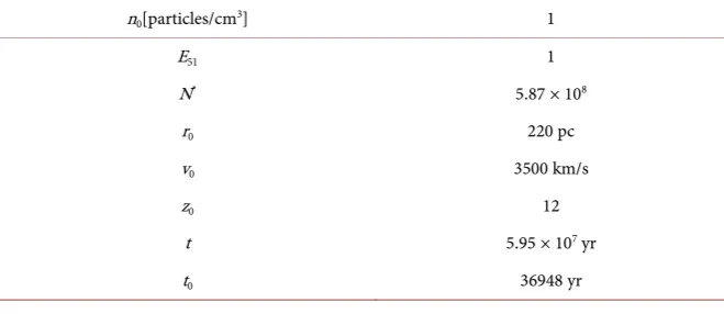
− z (16)A possible set of initial values is reported in Table 1 in which the initial value of radius and velocity are fixed by the bursting phase.
The above parameters allows to obtain an approximate expansion law as func-tion of time and polar angle
( )
2,1 BN,r t
BD
= (17)
[image:5.595.208.538.579.722.2]with
Table 1. Numerical values of the parameters for the simulation in the case of the inverse square model.
n0[particles/cm3] 1
E51 1
N* 5.87 × 108
r0 220 pc
v0 3500 km/s
z0 12
t 5.95 × 10⁷ yr
DOI: 10.4236/ijaa.2018.82015 205 International Journal of Astronomy and Astrophysics
( )
(
)
( )
( )
( )
(
)
(
(
( )
)
(
( )
( )
)
)
22 2
2
1 2
31944000 cos 18.8632 cos 5111040cos
1.0289 101376 220cos 12 21083040000 cos 24899.49 cos 3219955200cos 0.0073517 4210.27 102871295 ,
BN t
t
t t
t
θ θ θ
θ θ
θ θ
= + +
+ − − +
− + +
+ −
(18)
and
( )
10560cos 720.BD= θ − (19)
4. Astrophysical Results
This section introduces a test for the reliability of the model, analyzes the obser-vational details of the Fermi bubbles, reviews the results for the two models of reference and reports the results of the inverse square model.
4.1. The Reliability of the Model
An observational percentage reliability, obs, is introduced over the whole range of the polar angle θ,
obs num obs
obs,
100 1 j j many directions, j
j
r r
r
−
= −
∑
∑
(20)
where rnum is the theoretical radius, robs is the observed radius, and the index j varies from 1 to the number of available observations. In our case the observed radii are reported in Figure 2.
4.2. The Structure of the Fermi Bubbles
The exact shape of the Fermi bubbles is a matter of research and as an example in [38] the bubbles are modeled with ellipsoids centered at 5 kpc up and below the Galactic plane with semi-major axes of 6 kpc and minor axes of 4 kpc. In or-der to test our models we selected the image of the Fermi bubbles available at
https://www.nasa.gov/mission_pages/GLAST/news/new-structure.html which is reported in Figure 1. A digitalization of the above advancing surface is reported in Figure 2 as a 2D section. The actual shape of the bubbles in galactic coordi-nates is shown in Figure 3 and Figure 15 of [4] and Figure 30 and Table 3 of by
[39].
4.3. The Two Models of Reference
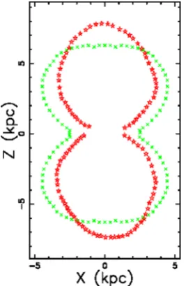
The thermal model is outlined in Section 3.1 and Figure 3 reports the numerical solution as a cut in the x-z plane.
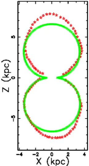
The cold recursive model is outlined in Section 3.2 and Figure 4 reports the numerical solution as a cut in the x-z plane.
4.4. The Inverse Square Model
DOI: 10.4236/ijaa.2018.82015 206 International Journal of Astronomy and Astrophysics
[image:7.595.293.458.254.419.2]Figure 1. A gamma - X image of the Fermi bubbles in 2010 as given by the NASA.
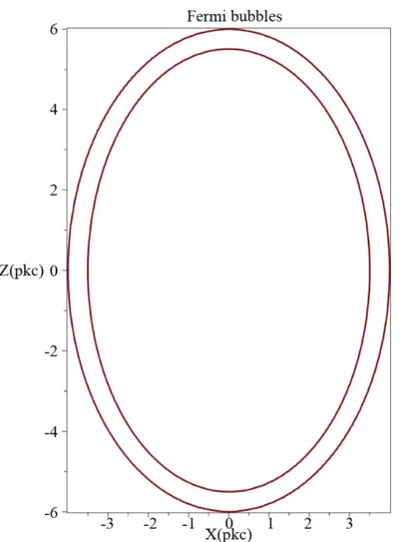
Figure 2. A section of the Fermi bubbles digitalized by the author.
Figure 3. Section of the Fermi bubbles in the x z− plane with a thermal model (green points) and observed profile (red stars). The bursting parameters N* = 113,000,
OB
z = 0 pc, E51 = 1, t0= 0.036 10 yr× 7 when t= 90 10 yr× 7 give
obs= 73.34%
[image:7.595.308.442.452.657.2]DOI: 10.4236/ijaa.2018.82015 207 International Journal of Astronomy and Astrophysics
Figure 4. Section of the Fermi bubbles in the x z− plane with the cold recursive model (green points) and observed profile (red stars). The bursting parameters N* = 79,000,
OB
z = 2 pc, 7
0= 0.013 10
t × yr and
51
E = 1 gives r0= 90.47 pc and v0= 391.03 km∙s−1. On inserting = 90
h pc, t= 13.6 10× 7 yr the reliability is
obs= 84.70%
[image:8.595.311.440.67.317.2]ε .
[image:8.595.301.446.404.673.2]DOI: 10.4236/ijaa.2018.82015 208 International Journal of Astronomy and Astrophysics
numerical solution as a cut in the x-z plane.
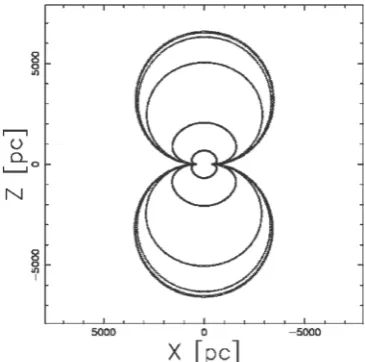
[image:9.595.233.513.145.435.2]A rotation around the z-axis of the above theoretical section allows building a 3D surface, see Figure 6. The temporal evolution of the advancing surface is re-ported in Figure 7 and a comparison should be done with Figure 6 in [40].
Figure 6. 3D surface of the Fermi bubbles with parameters as in Table 1, inverse square profile. The three Euler angles are Θ= 40, Φ= 60 and
= 60
Ψ .
Figure 7. Sections of the Fermi bubbles as function of time with parameters as in Table 1. The time of each section is 0.0189 10 yr× 7 , 0 059 10 r. × 7y ,
7
[image:9.595.282.465.492.673.2]DOI: 10.4236/ijaa.2018.82015 209 International Journal of Astronomy and Astrophysics
5. Theory of the Image
This section reviews the transfer equation and reports a new analytical result for the intensity of radiation in an elliptical framework in the non-thermal/thermal case. A numerical model for the image formation of the Fermi bubbles is re-ported.
5.1. The Transfer Equation
The transfer equation in the presence of emission only in the case of optically thin layer is
( )
,jνρ=KC s (21)
where K is a constant, jν is the emission coefficient, the index ν denotes the
frequency of emission and C s
( )
is the number density of particles, see for example [41]. As an example the synchrotron emission, as described in sec. 4 of[42], is often used in order to model the radiation from a SNR, see for example
[43][44][45]. According to the above equation the increase in intensity is pro-portional to the number density integrated along the line of sight, which for constant density, gives
,
Iν =K l′× (22)
where
K
′
is a constant and l is the length along the line of sight interested inthe emission; in the case of synchrotron emission see Formula (1.175) in [46].
5.2. Analytical Non Thermal Model
A real ellipsoid, see [47], represents a first approximation of the Fermi bubbles, see [38], and has equation
2 2 2
2 2 2 1,
z x y
a +b +d = (23)
in which the polar axis of the Galaxy is the z-axis. Figure 8 reports the astro-physical application of the ellipsoid in which due to the symmetry about the azimuthal angle b d= .
We are interested in the section of the ellipsoid y=0 which is defined by the
following external ellipse
2 2
2 2 1.
z x
a +b = (24)
We assume that the emission takes place in a thin layer comprised between the external ellipse and the internal ellipse defined by
(
) (
)
2 2
2 2 1,
z x
a c− + b c− = (25)
see Figure 9 We therefore assume that the number density C is constant and in particular rises from 0 at (0, a) to a maximum value Cm, remains constant up to
DOI: 10.4236/ijaa.2018.82015 210 International Journal of Astronomy and Astrophysics
Figure 8. Fermi bubbles approximated by an ellipsoid when 6kpc, 4kpc and 4kpc
a= b= d= .
Figure 9. Internal and external ellipses when a= 6kpc, = 4kpc
b and = kpc
[image:11.595.262.485.379.681.2]DOI: 10.4236/ijaa.2018.82015 211 International Journal of Astronomy and Astrophysics
the position z in a Cartesian x-z plane and terminates at the external ellipse. The locus length is
2 2
2
I a z b
l
a
−
= (26)
when
(
a c−)
≤ <z a(
)
2 2 2
2 2 2
2 2
II
a ac c z b c a z b
l
a a c
− + − −
−
= −
− (27)
when 0≤ <z
(
a c−)
.In the case of optically thin medium, according to equation (22), the intensity is split in two cases
(
; ,)
2 2 2I m a z b
I z a b I
a
−
= × (28)
when
(
a c−)
≤ <z a(
; ,)
2 2 2 2 2 2 2 2(
)
II m
a ac c z b c
a z b I z a c I
a a c
− − + − −
= × −
−
(29)
when 0≤ <z
(
a c−)
,where Im is a constant which allows to compare the theoretical intensity with
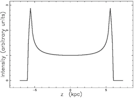
the observed one. A typical profile in intensity along the z-axis is reported in
Figure 10. The ratio, r, between the theoretical intensity at the maximum,
(
z a c= −)
, and at the minimum, (z
=
0
), is given by(
)
(
0)
2 .I
II
I z a c a cb r
I z ca
= − −
= =
= (30)
As an example the values a=6 kpc, b=4 kpc, kpc 12
a
c= gives
r
=
3.19
.The knowledge of the above ratio from the observations allows to deduce c once
[image:12.595.209.531.108.208.2] [image:12.595.260.490.506.677.2]a and b are given by the observed morphology
Figure 10. The intensity profile along the z-axis when when = 6kpc
a , b= 4kpc and = kpc 12
a
DOI: 10.4236/ijaa.2018.82015 212 International Journal of Astronomy and Astrophysics 2
2 2 2
2 ab .
c
a r b
=
+ (31)
As an example in the inner regions of the northeast Fermi bubble we have
2
r= , see [6], which coupled with a=6 kpc and b=4 kpc gives 1.2 kpc
c= . The above value is an important astrophysical result because we have found the dimension of the advancing thin layer.
5.3. Analytical Thermal Model
A thermal model for the image is characterized by a constant temperature in the internal region of the advancing section which is approximated by an ellipse, see equation (24). We therefore assume that the number density C is constant and in particular rises from 0 at (0, a) to a maximum value Cm, remains constant up to
(0, −a) and then falls again to 0. The length of sight, when the observer is si-tuated at the infinity of the x-axis, is the locus parallel to the x-axis which crosses the position z in a Cartesian x-z plane and terminates at the external ellipse in the point (0,a). The locus length is
2 2
2 a z b; .
l a z a a
−
= − ≤ < (32)
The number density Cm is constant in the ellipse and therefore the intensity of
radiation is
(
; , , m)
m 2 a2 z b2 ; .I z a b I I a z a a
−
= × − ≤ < (33)
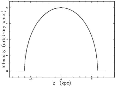
A typical profile in intensity along the z-axis for the thermal model is reported in Figure 11.
5.4. Numerical Model
The source of luminosity is assumed here to be the flux of kinetic energy, Lm,
[image:13.595.258.489.511.682.2]DOI: 10.4236/ijaa.2018.82015 213 International Journal of Astronomy and Astrophysics 3
1 ,
2
m
L = ρAV (34)
where A is the considered area, V the velocity and
ρ
the density, see formula (A28) in [48]. In our case A R= ∆Ω2 , where ∆Ω is the considered solid angle along the chosen direction. The observed luminosity along a given direction can be expressed as, m
L=L (35) where is a constant of conversion from the mechanical luminosity to the ob-served luminosity. A numerical algorithm which allows us to build a complex image is outlined in Section 4.1 of [49] and the orientation of the object is cha-racterized by the Euler angles
(
Φ Θ Ψ, ,)
The threshold intensity can be para-metrized to Imax, the maximum value of intensity characterizing the map. The image of the Fermi bubbles is shown in Figure 12 and the introduction of thre-shold intensity is visualized in Figure 13.6. Conclusions
Law of motion. We have compared two existing models for the temporal evolu-tion of the Fermi bubbles, a thermal model, see Secevolu-tion 3.1, and an autogravitat-ing model, see Section 3.2, with a new model which conserves the momentum in presence of an inverse square law for the density of the ISM. The best result is obtained by the inverse square model which produces a reliability of
obs=90.71%
for the expanding radius in respect to a digitalized section of the Fermi bubbles. A semi-analytical law of motion as function of polar angle and time is derived for the inverse square model, see Equation (17).
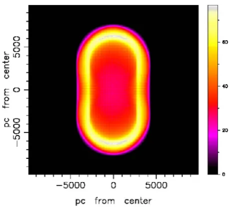
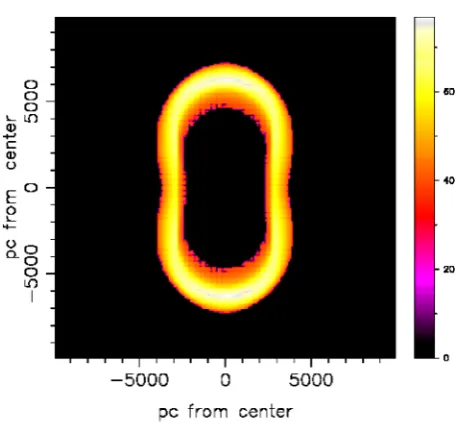
Figure 12. Map of the theoretical intensity of the Fermi bubbles for the inverse square model with parameters as in
[image:14.595.258.488.454.662.2]DOI: 10.4236/ijaa.2018.82015 214 International Journal of Astronomy and Astrophysics
Figure 13. Map of the theoretical intensity of the Fermi bubbles as in Figure 1. In this map Itr=Imax 2.
Formation of the image. An analytical cut for the intensity of radiation along the z-axis is derived in the framework of advancing surface characterized by an internal and an external ellipsis. The analytical cut in theoretical intensity presents a characteristic “U” shape which has a maximum in the external ring and a minimum at the center, see Equation (30). The presence of a hole in the intensity of radiation in the central region of the elliptical Fermi bubbles is also confirmed by a numerical algorithm for the image formation, see Figure 13. The theoretical prediction of a hole in the intensity map explains the decrease in in-tensity for the 0.3 kev plasma by = 50% toward the central region of the north-east Fermi bubble, see [6]. The intensity of radiation for the thermal model con-versely presents a maximum of the intensity at the center of the elliptical Fermi bubble, see Equation (33) and this theoretical prediction does not agree with the above observations.
Acknowledgements
Credit for Figure 1 is given to NASA.
References
[1] Heiles, C. (1979) H I Shells and Supershells. The Astrophysical Journal, 229, 533.
https://doi.org/10.1086/156986
[2] Pikel’Ner, S.B. (1968) Interaction of Stellar Wind with Diffuse Nebulae. The Astro-physical Journal Letters, 2, 97.
[3] Weaver, R., McCray, R., Castor, J., Shapiro, P. and Moore, R. (1977) Interstellar bubbles. II—Structure and Evolution. The Astrophysical Journal, 218, 377.
https://doi.org/10.1086/155692
[image:15.595.259.490.63.274.2]DOI: 10.4236/ijaa.2018.82015 215 International Journal of Astronomy and Astrophysics
https://doi.org/10.1088/0004-637X/724/2/1044
[5] Jones, D.I., Crocker, R.M., Reich, W., et al. (2012) Magnetic Substructure in the Northern Fermi Bubble Revealed by Polarized Microwave Emission. The Astro-physical Journal, 747, L12. (Preprint) https://doi.org/10.1088/2041-8205/747/1/L12
[6] Kataoka, J., Tahara, M., Totani, T., et al. (2013) Suzaku Observations of the Diffuse X-Ray Emission across the Fermi Bubbles’ Edges. The Astrophysical Journal, 779, 57. (Preprint) https://doi.org/10.1088/0004-637X/779/1/57
[7] Tahara, M., Kataoka, J., Takeuchi, Y., et al. (2015) Suzaku X-Ray Observations of the Fermi Bubbles: Northernmost Cap and Southeast Claw Discovered with MAXI-SSC. The Astrophysical Journal, 802, 91. (Preprint)
https://doi.org/10.1088/0004-637X/802/2/91
[8] Kataoka, J., Tahara, M., Totani, T., et al. (2015) Global Structure of Isothermal Dif-fuse X-Ray Emission along the Fermi Bubbles. The Astrophysical Journal, 807, 77. (Preprint) https://doi.org/10.1088/0004-637X/807/1/77
[9] Fox, A.J., Bordoloi, R., Savage, B.D., et al. (2015) Probing the Fermi Bubbles in Ul-traviolet Absorption: A Spectroscopic Signature of the Milky Way’s Biconical Nuc-lear Outflow. The Astrophysical Journal, 799, L7. (Preprint)
https://doi.org/10.1088/2041-8205/799/1/L7
[10] Bordoloi, R., Fox, A.J., Lockman, F.J., et al. (2017) Mapping the Nuclear Outflow of the Milky Way: Studying the Kinematics and Spatial Extent of the Northern Fermi Bubble. The Astrophysical Journal, 834, 191. (Preprint)
https://doi.org/10.3847/1538-4357/834/2/191
[11] Abeysekara, A.U., Albert, A., Alfaro, R., et al. (2017) Search for Very High-Energy Gamma Rays from the Northern Fermi Bubble Region with HAWC. The Astro-physical Journal, 842, 85. (Preprint) https://doi.org/10.3847/1538-4357/aa751a
[12] Cheng, K.S., Chernyshov, D.O., Dogiel, V.A., et al. (2011) Origin of the Fermi Bub-ble. The Astrophysical Journal, 731, L17. (Preprint)
https://doi.org/10.1088/2041-8205/731/1/L17
[13] Yang, H.Y.K., Ruszkowski, M., Ricker, P.M., et al. (2012) The Fermi Bubbles: Su-personic Active Galactic Nucleus Jets with Anisotropic Cosmic-Ray Diffusion. The Astrophysical Journal, 761, 185. (Preprint)
https://doi.org/10.1088/0004-637X/761/2/185
[14] Fujita, Y., Ohira, Y. and Yamazaki, R. (2013) The Fermi Bubbles as a Scaled-Up Version of Supernova Remnants. The Astrophysical Journal, 775, L20. (Preprint)
https://doi.org/10.1088/2041-8205/775/1/L20
[15] Thoudam, S. (2013) Fermi Bubble γ-Rays as a Result of Diffusive Injection of Ga-lactic Cosmic Rays. The Astrophysical Journal, 778, L20. (Preprint)
https://doi.org/10.1088/2041-8205/778/1/L20
[16] Fujita, Y., Ohira, Y. and Yamazaki, R. (2014) A Hadronic-Leptonic Model for the Fermi Bubbles: Cosmic-Rays in the Galactic Halo and Radio Emission. The Astro-physical Journal, 789, 67.
[17] Cheng, K.S., Chernyshov, D.O., Dogiel, V.A. and Ko, C.M. (2015) Multi-Wavelength Emission from the Fermi Bubble. II. Secondary Electrons and the Hadronic Model of the Bubble. The Astrophysical Journal,799, 112.
[18] Sasaki, K., Asano, K. and Terasawa, T. (2015) Time-Dependent Stochastic Accelera-tion Model for Fermi Bubbles. The Astrophysical Journal,814, 93.
DOI: 10.4236/ijaa.2018.82015 216 International Journal of Astronomy and Astrophysics [20] Crocker, R.M., Bicknell, G.V., Carretti, E., et al. (2014) Steady-State Hadronic
Gamma-Ray Emission from 100-Myr-Old Fermi Bubbles. The Astrophysical Jour-nal Letters,791, L20.
[21] Lockman, F.J. (1984) The H I Halo in the Inner Galaxy. The Astrophysical Journal, 283, 90-97.
[22] Dickey, J.M. and Lockman, F.J. (1990) H I in the Galaxy. Annual Review of As-tronomy and Astrophysics,28, 215-259.
[23] Bisnovatyi-Kogan, G.S. and Silich, S.A. (1995) Shock-Wave Propagation in the Nonuniform Interstellar Medium. Reviews of Modern Physics,67, 661.
https://doi.org/10.1103/RevModPhys.67.661
[24] Zhu, H., Tian, W., Li, A. and Zhang, M. (2017) The Gas-to-Extinction Ratio and the Gas Distribution in the Galaxy. Monthly Notices of the Royal Astronomical Society, 471, 3494-3528.
[25] Spitzer, L. (1942) The Dynamics of the Interstellar Medium. III. Galactic Distribu-tion. The Astrophysical Journal,95, 329. https://doi.org/10.1086/144407
[26] Rohlfs, K. (1977) Lectures on Density Wave Theory. In: Lecture Notes in Physics, Vol. 69, Springer Verlag, Berlin.
[27] Bertin, G. (2000) Dynamics of Galaxies. Cambridge University Press, Cambridge. [28] Padmanabhan, P. (2002) Theoretical Astrophysics. Vol. III: Galaxies and
Cosmolo-gy. Cambridge University Press, Cambridge, UK.
[29] McCray, R.A. (1987) Coronal Interstellar Gas and Supernova Remnants. In: Dal-garno, A. and Layzer, D., Eds., Spectroscopy of Astrophysical Plasmas, Cambridge University Press, Cambridge, 255-278.
https://doi.org/10.1017/CBO9780511564659.011
[30] Dyson, J.E. and Williams, D.A. (1997) The Physics of the Interstellar Medium. In-stituteof Physics Publishing, Bristol. https://doi.org/10.1887/075030460X
[31] McCray, R. and Kafatos, M. (1987) Supershells and Propagating Star Formation.
The Astrophysical Journal,317, 190-196.
[32] Zaninetti, L. (2004) On the Shape of Superbubbles Evolving in the Galactic Plane.
Publications of the Astronomical Society of Japan,56, 1067.
[33] Zaninetti, L. (2012) Evolution of Superbubbles in a Self-Gravitating Disk. Monthly Notices of the Royal Astronomical Society, 425, 2343-2351.
[34] Padé, H. (1892) Sur la représentation approchée d’une fonction par des fractions ra-tionnelles. Annales Scientifiques de l’École Normale Supérieure, 9, 193.
[35] Olver, F.W., Lozier, D.W., Boisvert, R.F. and Clark, C.W. (2010) NIST Handbook of Mathematical Functions. Cambridge University Press, Cambridge.
[36] Baker, G. (1975) Essentials of Padé Approximants. Academic Press, New York. [37] Baker, G.A. and Graves-Morrism, P.R. (1996) Padé Approximants. Vol. 59,
Cam-bridge University Press, CamCam-bridge. https://doi.org/10.1017/CBO9780511530074
[38] Miller, M.J. and Bregman, J.N. (2016) The Interaction of the Fermi Bubbles with the Milky Way’s Hot Gas Halo. The Astrophysical Journal,829, 9.
[39] Ackermann, M., Albert, A., Atwood, W.B., et al. (2014) The Spectrum and Mor-phology of the Fermi Bubbles. The Astrophysical Journal,793, 64.
Wi-DOI: 10.4236/ijaa.2018.82015 217 International Journal of Astronomy and Astrophysics ley-Interscience, New York.
[42] Schlickeiser, R. (2002) Cosmic Ray Astrophysics. Springer, Berlin.
https://doi.org/10.1007/978-3-662-04814-6
[43] Yamazaki, R., Ohira, Y., Sawada, M. and Bamba, A. (2014) Synchrotron X-Ray Di-agnostics of Cutoff Shape of Nonthermal Electron Spectrum at Young Supernova Remnants. Research in Astronomy and Astrophysics, 14, 165-178.
https://doi.org/10.1088/1674-4527/14/2/005
[44] Tran, A., Williams, B.J., Petre, R., Ressler, S.M. and Reynolds, S.P. (2015) Energy Dependence of Synchrotron X-Ray Rims in Tycho’s Supernova Remnant. The As-trophysical Journal,812, 101.
[45] Katsuda, S., Acero, F., Tominaga, N., Fukui, Y., Hiraga, J.S., Koyama, K., Lee, S.H., Mori, K., Nagataki, S., Ohira, Y., Petre, R., Sano, H., Takeuchi, Y., Tamagawa, T., Tsuji, N., Tsunemi, H. and Uchiyama, Y. (2015) Evidence for Thermal X-Ray Line Emission from the Synchrotron-Dominated Supernova Remnant RX J1713.7-3946.
The Astrophysical Journal,814, 29.
[46] Lang, K.R. (1999) Astrophysical Formulae. 3rd Edition, Springer, New York. [47] Zwillinger, D. (2018) CRC Standard Mathematical Tables and Formulas, 33rd
Edi-tion. In: Advances in Applied Mathematics, CRC Press, New York.
[48] De Young, D.S. (2002) The Physics of Extragalactic Radio Sources. University of Chicago Press, Chicago.