Autonomous Learning Multi-Model Systems from
Data Streams
Plamen P. Angelov,
Fellow, IEEE
, Xiaowei Gu,
Student Member, IEEE
, and Jos´e C. Pr´ıncipe,
Fellow, IEEE
Abstract—In this paper, an approach to autonomous learning of a multi-model system from streaming data, named ALMMo, is proposed. The proposed approach is generic and can easily be applied also to probabilistic or other types of local models forming multi-model systems. It is fully data-driven and its structure is decided by the nonparametric data clouds extracted from the empirically observed data without making any prior assumptions concerning data distribution and other data prop-erties. All meta-parameters of the proposed system are obtained directly from the data and can be updated recursively, which improves memory- and calculation-efficiency of the proposed algorithm. The structural evolution mechanism and online data cloud quality monitoring mechanism of the ALMMo system largely enhance the ability of handling shifts and/or drifts in the streaming data pattern. Numerical examples of the use of ALMMo system for streaming data analytics, classification and prediction are presented as a proof of the proposed concept.
Index Terms—autonomous learning systems, AnYa type fuzzy rule-based system, Empirical Data Analytics, data clouds, non-parametric, classification, prediction.
I. INTRODUCTION
AUTONOMOUS Learning Systems (ALSs) [1] can be seen as the physical embodiments of machine intelligence. An ALS can also be seen as a fusion of computationally enabled sensor platforms (machines/devices) that possess the algorithms (respectively, the software) needed to empower the systems with evolving intelligence that is manifested through interaction with the outside environment and self-monitoring. The core characteristics of any ALS are the self-monitoring and self-adaption. Autonomous learning and extracting new knowledge as well as updating the existing knowledge base are, thus, vitally important [1].
A very efficient structural form for the ALSs is the multiple model architecture [2]–[4]. Multiple models can be used to describe different operating regimes, local specifics using simple local models (e.g. linear, Gaussian, singleton, etc.) [1]– [4]. An example of a multi-model system is the fuzzy rule-based (FRB) system [5]–[10]. It has been theoretically proven
Manuscript received December 2016. This work was partially supported by The Royal Society grant IE 141329/2014 ”Novel Machine Learning Paradigms to address Big Data Streams”.
Corresponding Author: Xiaowei Gu
Plamen P. Angelov is with School of Computing and Communication-s, Lancaster University, Lancaster, LA1 4WA., and also holds an Hon-orary Professor title with Technical Unviersity, Sofia, Bulgaria (e-mail: [email protected])
Xiaowei Gu is with School of Computing and Communications, Lancaster University, Lancaster, LA1 4WA. (e-mail: [email protected]).
Jos´e C. Pr´ıncipe is with Computational NeuroEngineering Laboratory, Depart-ment of Electrical and Computer Engineering, University of Florida, USA. (e-mail: [email protected]).
that both, the artificial neural networks (ANNs) [11] and the FRB systems [12] are universal approximators. Nonetheless, handcrafting an effective multiple model system currently requires a significant human expertise and efforts [2], [3], [5]– [8].
In this paper, we introduce a new fully autonomous learning system for streaming data, named ALMMo. In the proposed
ALMMosystem, the structure is composed of constraints-free
data cloudsforming Voronoi tessellation [13] in terms of the input and output variables. Its structure identification concerns the identification of the focal points of thedata cloudsas well as the parameters of output local models. Correspondingly, the parameter identification problem of the proposed approach is to determine the optimal values of the consequent parameters of the local (linear or singleton) models [1], [9].
The proposedALMMosystem can also be viewed as an au-tonomously self-developing AnYa type FRB system designed using the principles and mechanisms of the recently introduced Empirical Data Analytics (EDA) computational framework [10], [14]. Specific characteristics that setALMMoapart from the existing methods and schemes include:
1) it employs the nonparametric EDA quantities ofdensity
andtypicalityto disclose the underlying data pattern of the streaming data (note that “nonparametric” means that there is no model with parameters imposed for the data generation, it also means no user- or problem- specific parameters, but this does not mean that our algorithms do not have meta-parameters to achieve data processing); 2) its system structure is composed of data clouds free from external constraints and self-updating output local models identified in a data-driven way;
3) it further defines and identifies aunimodal densitybased membership function [10] designed within the EDA framework to the AnYa type FRB system [9];
4) it can, in a natural way, deal with heterogeneous data combining categorical with continuous data [10].
higher and not limited by these illustrative examples.
II. ALMMOSTRUCTURE,DATA CLOUDSAND THE EDA FRAMEWORK
A. Multi-Model Systems
Multi-model systems have been used for decades in adaptive control, observers, predictors, classifiers [2], [3], [15] as a powerful tool able to handle problems with both measurement and motion uncertainties. Multi-model systems exploit the centuries’ old principle of “divide and rule” [1]–[4], [7] by decomposing complex problems into a set of simpler ones and combining these afterwards. Examples of multi-model systems include but are not limited to FRB systems [1], [7].
FRB systems consist of a number of fuzzy rules representing the local areas of the data space. There are two widely used types of FRB systems, namely, i) the Mamdani type [5], [6] and ii) the Takagi-Sugeno type [7], [8]. The antecedent part of a Mamdani or Takagi-Sugeno type fuzzy rule is determined by a number of fuzzy sets (one per variable), which are them-selves defined by parameterized scalar membership functions, e.g. triangular, trapezoidal or Gaussian. There are, in general, two approaches to identify the membership functions, namely,
i)human expertise-based, andii)clustering-based approaches. However, a number of issues arise when identifying antecedent parts [9], [10]:
1) Defining a membership function requires ad hoc deci-sions;
2) Membership functions often differ significantly from the real data distribution;
3) “Curse of dimensionality”.
An illustrative example of a FRB system designed by human experts and a clustering-based FRB system is depicted in the supplementary Fig. 1.
The proposed ALMMo system employs the nonparametric EDA quantities (density andtypicality), which will be briefly recalled in the next subsection to disclose the underlying data pattern of the streaming data, and based on which formsdata cloudsused as the antecedent (IF) part of its AnYa type fuzzy rules in a data-driven way. In ALMMo, each local model is associated with a certaindata cloud. This method of forming
data clouds is different from the eClustering method used in the original AnYa paper [9].
AnYa type FRB system was recently introduced aiming to simplify the antecedent parts of the fuzzy rules [1], [9], which are uniquely defined by focal points of the nonparametric, constraint-free data clouds consisting of the data samples associated with the nearest focal points. AnYa type FRB is closely linked with the concept of data clouds introduced in [1], [9].
Data cloudsare very much like clusters, but differ in several aspects. They are nonparametric, free from external constraints and do not have a specific shape. They directly represent the local ensemble properties of the observed data samples. In contrast, the traditional pdfs [16] or membership functions used in fuzzy set theory [5]–[7] often do not represent the true data distributions and, instead, represent some desir-able/expected/estimated or subjective preferences in the case
of fuzzy membership functions. Data clouds consist of the data samples affiliated with the nearest focal points resembling Voronoi tessellation [13]. The visual example ofdata clouds
based on the UCI benchmark dataset Banknote Authentication [17] is presented in Fig. 1, where the dots in different colors are the members of different data clouds, the black asterisks are the focal points. For visual clarity, we only present the first two attributes of the dataset, namely, variance and skewness of wavelet-transformed image. As we can clearly see from the figure, thedata clouds do not have specific shapes, their boundaries are decided by their mutual distribution.
-6 -4 -2 0 2 4 6
Variance of wavelet transformed image -10
-5 0 5 10
[image:2.612.319.543.209.368.2]Skewness of wavelet transformed image
Fig. 1: Example ofdata cloudsbased on real data.
All data samples are assigned to the nearest focal points formingdata clouds. One can then easily formulate the follow-ing rule describfollow-ing the data clouds structure and assignment process:
IF(j∗= argmin
i=1,2,...,N
(||x−µi||))THEN(Ξj∗←x), (1)
where x = [x1, ..., xM]T is a particular data sample in the
Euclidean data space RM; Ξi denotes the ith data cloud andµi is the corresponding center;N is the number of data
clouds/local modes of the observed data samples inRM, also is the number of fuzzy rules in the FRB system.
The proposed ALMMosystem also replaces the commonly usedad hoc membership functions with theunimodal density
based membership function [10]. This improvement signifi-cantly reduces the efforts of human experts and, at the same time, largely enhances the objectiveness of the FRB system. In this sense, the proposed approach differs from the original AnYa [9] as well.
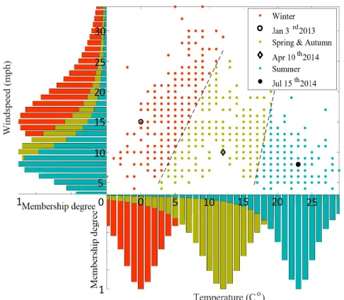
the three data clouds in Fig. 2 representing Winter, Summer and Spring/Autumn. However, these data clouds were not predefined, they emerged from the data.
Fig. 2: Visualization of the partitioning result and2D unimodal density based membership function of the climate dataset.
The structure of the proposed ALMMo system is depicted in Fig. 3 and is described as follows [1], [9]:
Fig. 3: A simple sketch diagram of the proposed ALMMo
system.
IF(x∼Ξj)THEN(yj =uTaj); (2) y=
N
X
j=1
λjuTaj=ΨTA, (3)
where Ξj denotes the jth data cloud, j = 1,2, ..., N; yj is the output of the jth fuzzy rule; uT = [1,xT] =
[1, x1, ..., xM];y is the overall output of theALMMosystem;
aj is the consequent parameters of the jth fuzzy rule, aj =
[aj,0, aj,1, aj,M]T;λj is the activation level of the jth fuzzy
rule; Ψ= [λ1uT, λ2uT, ..., λNuT]T;A= [aT1,aT2, ...,aTN]T. As it was stated before, one of the main novelties of this paper is the proposed identification ofALMMowithin the EDA framework. We will then briefly introduce the concept of EDA.
B. EDA Framework
Empirical Data Analytics (EDA) framework was introduced recently [14] as a new methodology for data analytics, which is free from pre-defined parameters and assumptions. The main problem addressed by the EDA framework is to estimate the ensemble properties of data based on the given observations of outcomes of actual processes/experiments alone. Therefore, the individual data samples do not need to be independent or identically distributed (i.i.d.) as in the traditional statistics [19], [20]; on the contrary, their mutual dependence is taken into account directly through the mutual distances between the data points/samples. The main nonparametric EDA quantities used in this paper include:
i) Unimodal discrete density,D [14];
ii) Multimodal continuous typicality,τM M [21].
Let us assume the collection of the observed data sam-ples of the data stream in RM are denoted by {x}
K = {x1,x2, ...,xK} (xi = [xi,1, xi,2, ..., xi,M]T ∈ RM, i =
1,2, ..., K), where the subscripts indicate the time instances at which data samples were observed and only one data sample arrives at each time instance.
i) Unimodal discrete density,D
Unimodal discrete density, D is derived directly from the ensemble properties and mutual distributions of observed data samples. It concerns the spatial distribution at a particular data sample in regards to all other data samples. It is defined generally for any type of distance. For the most common Euclidean type of distance, theunimodal discrete densitygets the form of a Cauchy function. Theunimodal discrete density
of the data samplex(x∈ {x}K) is defined as [14] :
DK(x) =
1
1 +||x−µK||2
σ2
K
, (4)
where σ2
K = XK− ||µK||2; µK andXK are, respectively, the mean and the average scalar product of the dataset{x}K, and they can be updated recursively as follows [1]:
µK= K−1
K µK−1+
1
KxK; µ1=x1; (5)
XK = K−1
K XK−1+
1
K||xK||
2; X
1=||x1||2. (6)
ii) Multimodal continuous typicality,τM M
Multimodal continuous typicality,τM M[21] ofxis defined as the weighted sum ofcontinuous multivariate Cauchy type kernel functions[22]–[24] corresponding to thedata clouds. An interesting property ofτM M is that it integrates to 1 [21]:
τKM M(x) = 1
K NK
X
i=1
SK,iκK,i(x), (7a)
where κK,i(x) is the multivariate Cauchy type kernel functionof the ithdata cloud and is expressed as:
κK,i(x) = Γ(
M+1 2 )
(πM2+1σM K,i(1 +
||x−µK,i||2
σ2
K,i
)M2+1)
[image:3.612.55.294.392.532.2]where i= 1,2, ..., NK;Γ(·)is the gamma function; πis the well-known constant;NK is the number of local modes at the Kth; SK,i is the number of data samples associated with the ith local mode and PNK
i=1SK,i = K holds; µK,i and σK,i
(σ2
K,i = XK,i − ||µK,i||2) are the mean and the standard deviation of the data samples within the ithdata cloud.
The multimodal continuous typicality, τM M provides an intuitive visualization of the empirically observed data pattern and is free from any pre-defined parameters. Nonetheless, it is worth to notice that themultivariate Cauchy type kernel functions being used in themultimodal continuous typicality
is not a prior assumption but a result of using Euclidean type distance.
Illustrative examples of the unimodal discrete density D and multimodal continuous typicality τM M are depicted in supplementary Fig. 2.
III. AUTONOMOUS LEARNING OF MULTI-MODEL SYSTEMS
In this section, we will describe the learning process of the ALMMo system, which includes the following two main stages: i) structure identification and ii) parameter identifi-cation. We will consider the well-known Euclidean distance without loss of generality (this system is not limited to Euclidean type only).
A. Structure (data clouds) Identification (divide and rule)
For each newly arrived data sample, denoted asxK+1, the
global mean and average scalar products µK and XK are updated to µK+1 and XK+1 firstly using equations (5) and
(6).
Theunimodal discrete densityatxK+1 and the focal points
of the existing data clouds µK,i (i = 1,2, ..., NK) are calculated using equation (4), denoted by DK+1(xK+1)and
DK+1(µK,i) (i = 1,2, ..., NK). The following principle is checked to see whether xK+1 will generate a new rule:
Cond.1:IF(DK+1(xK+1)> max
i=1,2,...,NK
(DK+1(µK,i)))
OR(DK+1(xK+1)< min
i=1,2,...,NK
(DK+1(µK,i)))
THEN (xK+1 is a new focal point).
(8)
If condition 1 is met, a new rule is added based around xK+1.
It is necessary to check whether the newdata cloudoverlaps with the existing data clouds, the following principle is used here to avoid possible overlaps:
Cond.2:IF(DK+1,i(xK+1)≥
1 1 +n2)
THEN
the ith focal point and the respective data cloud needs to be replaced by a new one
,
(9)
whereDK+1,i(xK+1)is theunimodal discrete density calcu-lated per rule (data cloud) using the following equation:
DK+1,i(xK+1) =
1
1 + S
2
K,i||xK+1−µK,i||2
(SK,i+1)(SK,iXK,i+||xK+1||2)−||xK+1+SK,iµK,i||2
. (10)
The rationale to consider DK+1,i(xK+1) ≥ 1/(1 +n2) comes from the well-known Chebyshev inequality [25] which describes the probability of a particular data samplex to be ntime standard deviation,σaway from the mean, µ:
P(||x−µ||2≤n2σ2)≥1− 1
n2. (11a)
Using theunimodal discrete density, the Chebyshev inequal-ity can be reformulated in a more elegant form as [14]:
P(DK+1,i(xK+1)≥ 1
1 +n2)≥1− 1
n2. (11b)
Here, we use n= 0.5. That is,DK+1,i(xK+1)≥0.8 for xK+1 is less than σ/2 away from the focal point of the ith data cloud. In other words, xK+1 is close to all points of
the ithdata cloud, therefore,xK+1 can replace theith focal
point.
If only Condition 1 is satisfied and Condition 2 is not met, a new rule (data cloud) with the focal point xK+1 is added:
NK+1←NK+ 1; (12a)
SK+1,NK+1 ←1; (12b)
µK+1,NK+1 ←xK+1; (12c)
XK+1,NK+1← ||xK+1||
2. (12d)
In contrast, if Conditions 1 and 2 are both satisfied, then the existing overlapping data cloud (assuming theithdata cloud) is being replaced by a new one with the focal pointxK+1 as
follows (NK+1←NK):
SK+1,i←
1 +SK,i
2
; (13a)
µK+1,i←
xK+1+µK,i
2 ; (13b)
XK+1,i←
||xK+1||2+XK,i
2 , (13c)
whered·edenotes the ceiling function.
The above principle is to prevent the ALMMo system from discarding the previously collected information too fast because the newdata cloudmay be initialized by an abnormal data sample.
If Condition 1 is not satisfied,xK+1is assigned to the
near-est existingdata cloudusing equation (1). The corresponding quantities are updated as follows (NK+1←NK):
SK+1,i←SK,i+ 1; (14a)
µK+1,i← SK,i SK+1,i
µK,i+ 1
SK+1,i
xK+1; (14b)
XK+1,i← SK,i SK+1,i
XK,i+ 1
SK+1,i
The descriptors (mean, scalar product and number of data samples) of the other data clouds stay the same for the next processing cycle. In ALMMo, each data cloud (and, the respective focal point) is used as a basis to formulate the antecedent (IF) part of the fuzzy rules.
B. Online Quality Monitoring
Since the proposedALMMosystem is for processing stream-ing data, monitorstream-ing the quality of the dynamically evolvstream-ing structure is necessary in order to guarantee efficiency. The quality of the fuzzy rules used in the ALMMo system can be characterized by their utility [1]. In the proposedALMMo
system, utility, ηK+1,i , accumulates the weight of the rule contributions to the overall output (activation level) during the life of the rule (from the moment when this rule was generated till the current time instance). It is the measure of importance of the respective fuzzy rule compared to the other rules (i= 1,2, ..., NK+1) [1], [9]:
ηK+1,i=
1
K+ 1−Ii K+1
X
l=Ii
λl,i; ηIi,i= 1, (15)
whereIiis the time instance at which theithdata cloud/fuzzy rule is established; λl,i is the activation level of ith data cloud/fuzzy rule at the lth time instance. In this paper, we define the activation level as the normalizedunimodal density
calculated per rule as (i= 1,2, ..., Nl):
λl,i= Dl,i(xl)
PNl
j=1Dl,j(xl)
. (16)
The rule base can be simplified according to the following principle by removing fuzzy rules (data clouds) with low
utility [1], [9]:
Cond.3:IF (ηK+1,j < η0)THEN(remove thejth fuzzy rule), (17) whereη0 is a small tolerance constant (in this paper, we use
η0= 0.1).
If thejthfuzzy rule satisfies Condition 3, it will be removed from the rule base and its consequent parametersCK+1,j and aK+1,j will be deleted as well.
C. Parameter Identification
At this stage, the consequent parameters of the ALMMo
system are updated.
If a new rule is added during the structure identification stage, the consequent parameters are set as follows.
aK,NK+1 ←
1
NK NK
X
j=1
aK,j; (18)
CK,NK+1←ΩI(M+1)×(M+1). (19)
If an old fuzzy rule (denoted as the jth rule) is replaced by a new one when the Conditions 1 and 2 are both satisfied, the new rule will inherit the consequent parameters of the old one.
After the structure of theALMMosystem is revised, we can use the fuzzy weighted RLS approach [26] or its modification fuzzy weighted generalized RLS method [27] to update the consequent parameters CK,j and aK,j (j = 1,2, ..., NK) locally:
CK+1,j =CK,j−
λK+1,jCK,juK+1uTK+1CK,j
1 +λK+1,juK+1CK,juTK+1
; (20)
aK+1,j =aK,j+λK+1,jCK+1,juK+1(yK+1−uTK+1aK,j),
(21) where aK,j, aK+1,j, CK,j and CK+1,j are the consequent parameters and co-variance matrix of thejthfuzzy rule at the
KthandK+1thtime instances, respectively;a
1,1= [
M+1
z }| {
0, ...,0]T andC1,1 =ΩI(M+1)×(M+1); Ω is a constant, in our paper,
Ω= 10is used.
D. Online Input Selection
In section II.B, we consider the dimension of input data samples to be M. However, in many practical cases, often there are a number of inter-correlated inputs. Therefore, it is very important to introduce the online input selection, which can further eliminate the waste of the computation- and memory-resources to improve the overall performance.
In this subsection, we add Condition 4 to deal with this [1]:
Cond.4:IF(ωK+1,i,j <ωK¯ +1,j)
THEN(remove thejth set from theithfuzzy rule), (22)
where j = 1,2, ..., M; i = 1,2, ..., NK+1 ; ωK+1,i,j is the normalized accumulated sum of parameter values at the time-instantK+ 1:
ωK+1,i,j =
qK+1,i,j
PM
j=1qK+1,i,j
; (23a)
¯
ωK+1,j is the average value of the normalized accumulated sum of thejth fuzzy set of all the rules:
¯
ωK+1,j =
PNK+1
i=1 ωK+1,i,j NK+1
; (23b)
is a constant parameter, ∈ [0.03,0.05]. The accumulated sum of parameter values, qK+1,i,j, is expressed as [1]:
qK+1,i,j = K+1
X
t=Ii
|at,i,j|, j = 1,2, ..., M. (23c)
If Condition 4 is met, we remove the corresponding fuzzy set from the rule and remove the corresponding column and row from the covariance matrixCK+1,j.
Finally, when the next data sample,xK+2comes, the system
output is generated as:
yK+2=
NK+1
X
j=1
λK+2,juTK+2aK+1,j. (24)
The learning process flowchart of the proposed ALMMo
Begin
Read the next data sample
Calculate ( ) by (16)
Generate system output by (24)
Update and by (5)-(6)
Condition 1
Delete the stale rules Condition 2
Add consequent parameters by
(18)-(19)
Inherit consequent parameters from the
old rule Replace the overlapping rule with
a new one by (13) Add a new rule
by (12)
Find the nearest data cloud by (1)
Update the meta-parameters by (14)
Calculate ( ) by (16)
Update ( ) by (15)
Condition 3
Condition 4
Remove the less important fuzzy sets
Update and ( ) by (20)-(21)
No
Yes
Yes
Yes
Yes No
No
[image:6.612.62.266.87.699.2]No
Fig. 4: Flowchart of the ALMMosystem’s learning process.
IV. APPLICATIONS OFALMMO
In this section, to test the proposed concepts and the method, we consider the following three applications of the proposed
ALMMolearning algorithm:
1) Online data analytics, structure identification and visu-alization;
2) Classification; 3) Prediction.
The overall performance of the proposed method is ana-lyzed based on comparisons with existing algorithms. Several benchmark datasets are used in the numerical experiments in this section. The algorithms were developed using MATLAB R2015a, performance was evaluated on a PC with processor 3.60 GHz×2, and 8 GB RAM.
A. Online Data Analytics
The proposed ALMMo system is able to perform online analytics on the streaming data thanks to its structural evo-lution mechanism. The system starts “from scratch” and quickly builds the data clouds/fuzzy rules directly from the observed data samples. With more data samples observed, the system begins to remove the stale fuzzy rules, which are not representative anymore and/or, at the same time, adds new fuzzy rules when the previously formed fuzzy rules do not represent the current data pattern well. By generating the
multimodal continuous typicality, τM M, the ALMMo system is able to provide a detailed and elegant visualization of the ever-changing data patterns of the observed streaming data.
The same climate dataset plotted in supplementary Figs. 1 and 2 is used to perform the online data analytics by the proposedALMMosystem, where the dataset is considered as a data stream.
The evolution ofdata cloudsand fuzzy rules generated by the ALMMo and the corresponding changes of focal points andmultimodal continuous typicalityare presented in a video in the Supplementary Materials, which is also downloadable from [28].
In this numerical experiment, we use η0 = 0.1. However,
due to the fact that a figure can only display 3-dimensional objects, we have to select two attributes, namely temperature and wind speed, for visualizing the multimodal continuous typicality.
B. Classification
In this subsection, we will consider the ALMMo based classification. For classification, we useη0= 0, which means
that, the system will not forget any knowledge gained during training, thus, ensure the fuzzy rules can cover the whole data stream.
Here, the normalized localunimodal discrete density (equa-tion (16)), which is generated per data cloud, is used as the basis function and the output class prediction by theALMMo
system. It is expressed as:
ˆ
y=
N
X
j=1
where the weights are defined as wj =uTaj,j = 1,2, ..., N. Thus, the class label can be determined by the output as:
Class(x) =Round(ˆy), (26)
where Round(ˆy) denotes the operation of rolling yˆ to the nearest integer.
The performance of the proposedALMMoclassifier is tested on the well-known challenging Pima dataset [29] with details tabulated in Table I. The attribute information is given in supplementary Table I. We have studied this dataset in [14] using the offline na¨ıve EDA based approaches. In this paper, we only involve the online approaches and the most popular offline ones for further comparison. The proposed classifier is compared with the following well-known approaches:
1) Self-organizing map (SOM) with winner takes all prin-ciple [30] with the net size9×9;
2) Learning vector quantization (LVQ) [31] with a hidden layer of size 32;
3) Back-propagation neural network (BPNN) with 3 hidden layers of size 16;
4) Na¨ıve Bayes classifier;
5) SVM with Gaussian kernel function (SVM-G) [32]; 6) SVM with linear kernel function (SVM-L) [32]; 7) FLEXFIS-Class [33];
8) Dynamic evolving neural-fuzzy inference system (DEN-FIS) [34];
9) Peephole long short-term memory (LSTM) [35], [36] with a hidden layer of size 32;
10) AnYa classifier [9]; 11) eClass0 [37];
12) Simpl eClass0 [38] and
13) Fuzzily connected multimodal systems (FCMMS) [4].
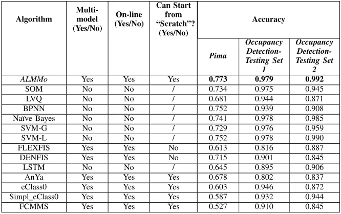
Note that among the comparative algorithms listed above, FLEXFIS-Class, DENFIS, AnYa classifier, eClass0, Sim-pl eClass0 and FCMS are the multi-model approaches. The proposedALMMoclassifier as well as AnYa classifier, eClass0, Simpl eClass0 and FCMS are evolving approaches which can start classifying “from scratch” from the very first data sample and self-evolve with the data stream, while the other classifiers require pre-training. In contrast with the original AnYa clas-sifier, the proposed ALMMoclassifier uses an advanced, non-parametric mechanism fordata cloud/fuzzy rule identification as well as the unimodal density-based membership functions as described earlier (see subsection III.A).
In this numerical example, 90% of the data samples are selected randomly for training and the rest are used for validation. For a fair comparison, we use pre-training for all classifiers. All the involved online approaches will stop learn-ing after the trainlearn-ing process. 30 Monte Carlo experiments are conducted and the average accuracies of the classification results are tabulated in Table II.
The confusion matrixes of the classification results obtained by selecting the first 90% (691 samples) of the dataset for training and using the rest of the data samples (77 samples) for validation are presented in supplementary Table II.
[image:7.612.333.538.68.209.2]We also conduct a comparison in an online scenario between the fully evolving algorithms that can start “from scratch”,
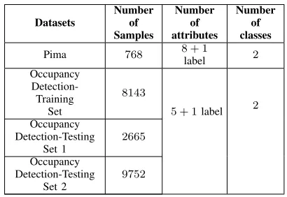
TABLE I: DETAILS OF THE BENCHMARK DATASETS
Datasets
Number of Samples
Number of attributes
Number of classes
Pima 768 8 + 1
label 2 Occupancy
Detection-Training
Set
8143
5 + 1label 2
Occupancy Detection-Testing
Set 1
2665
Occupancy Detection-Testing
Set 2
9752
TABLE III: OVERALL CLASSIFICATION PERFOR-MANCE COMPARISON ON BENCHMARK DATASETS-ONLINE SCENARIO
Algorithm Accuracy
Pima Occupancy Detection
ALMMo 0.751 0.986
AnYa 0.666 0.949
eClass0 0.570 0.931 Simpl eClass0 0.584 0.968 FCMMS 0.545 0.924
namely the proposed ALMMo classifier, AnYa classifier, e-Class0, Simpl eClass0 and FCMMS, by considering the Pima dataset as a data stream. In this experiment, the order of the data samples in the stream is randomly determined, and the algorithms start classifying from the first data sample and keep updating the system structure along with the arrival of new data samples. We repeated the experiment 30 times and report the average performance in Table III.
Further, another benchmark dataset (occupancy detection [39]) is also used for evaluation of the proposed approach. This dataset consists of one training set and two testing sets. Details of this dataset are tabulated in Table I and the attribute information is given in supplementary Table I.
In this numerical example, we firstly train the classifiers with the training set and conduct classification on the two testing sets separately with the trained classifiers in an offline scenario. 30 Monte Carlo experiments are conducted by ran-domly scrambling the order of the training samples and the overall accuracies of the classification results are presented in Table II. The average true positive rates and true negative rates of the classification results on the two testing sets obtained with the classifiers trained by the original training set are tabulated in supplementary Table III.
TABLE II: OVERALL CLASSIFICATION PERFORMANCE COMPARISON ON BENCHMARK DATASETS-OFFLINE SCENARIO
Algorithm
Multi-model (Yes/No)
On-line (Yes/No)
Can Start from “Scratch”?
(Yes/No)
Accuracy
Pima
Occupancy Detection-Testing Set
1
Occupancy Detection-Testing Set
2
ALMMo Yes Yes Yes 0.773 0.979 0.992
SOM No No / 0.734 0.975 0.945
LVQ No No / 0.681 0.944 0.871
BPNN No No / 0.752 0.939 0.908
Na¨ıve Bayes No No / 0.741 0.978 0.985
SVM-G No No / 0.729 0.976 0.959
SVM-L No No / 0.752 0.978 0.990
FLEXFIS Yes Yes No 0.613 0.816 0.887
DENFIS Yes Yes No 0.715 0.901 0.845
LSTM No No / 0.645 0.895 0.906
AnYa Yes Yes Yes 0.678 0.802 0.837
eClass0 Yes Yes Yes 0.603 0.946 0.872
Simpl eClass0 Yes Yes Yes 0.587 0.932 0.944
FCMMS Yes Yes Yes 0.527 0.910 0.845
the proposedALMMoclassifier is an online classifier and can work “from scratch”. The most important point is that the proposedALMMoclassifier is entirely data-driven and is free from unrealistic assumptions, restrictions or problem- or user-specific prior knowledge. In other studies, we also demon-strated thatALMMoclassifiers are able to achieve comparable or even better classification results against the state-of-the-art approaches in more complicated problems including, but not limited to, handwriting digital recognition, remote sensing image classification without the need of predefining (problem-or user- specific) parameters and thresholds [40].
C. Prediction
In this subsection, the performance of the online prediction using the proposed ALMMo system is reported. In the fol-lowing numerical examples, we use η0 = 0.1, which means
leaving out the rules that contribute less than 10%.
We consider a high frequency trading problem for testing the
ALMMopredictor. The data includes the QuantQuote Second Resolution Market Database [41], which contains tick-by-tick data on all NASDAQ, NYSE, and AMEX securities from 1998 to the present moment in time. The frequency of tick data varies from one second to few minutes. This dataset contains 19144 data samples. In this paper, we use the following attributes:
1) Time, K;
2) Open Price, xK,1;
3) High Price, xK,2;
4) Low Price, xK,3 and
5) Close Price, xK,4
for prediction of the future values of high price 8, 12, 16, 20 and 24 steps ahead, namelyyK =xK+8,2,yK =xK+12,2,
yK=xK+16,2,yK=xK+20,2andyK=xK+24,2,
respective-ly. The data samples are standardized online before prediction.
Firstly, we use xK as the input to predict the high price 8 steps ahead, xK+8,2. The overall prediction result is
p-resented in Fig. 5a and the evolution of number of data clouds/local modes/fuzzy rules is depicted in Fig. 5b. Three zoom-in periods (circulated areas in Fig. 5) are depicted in supplementary Figs. 3a-3c. Three of the fuzzy rules of the
ALMMo system in the final time instance are presented in Table IV as illustrative examples. The complete fuzzy rule set is given in supplementary Table IV. Note that the values of xK,1,xK,2,xK,3 andxK,4 presented in the fuzzy rules in the
two tables have been denormalized using the corresponding mean and standard deviation values.
As we can see from Fig. 5, there are many abnormal data samples and random fluctuations in the data stream. At the beginning and the end of this data stream, large fluctuations and abnormal data frequently appear, while in the middle, the data pattern changes relatively smoothly with only a small number of abnormal data. The corresponding changes of the system structure can also be seen in Fig. 5. Thus, one can see that, the proposed ALMMo predictor is capable to successfully follow the non-stationary data pattern and exhibits very accurate prediction results and demonstrates a strong evolving ability.
To study the performance of the proposedALMMopredictor, more experiments have been done and tabulated in Table V. Here, we additionally use the following algorithms for comparison:
1) FCMMS [4]; 2) AnYa [9];
3) Least square linear regression (LSLR) algorithm [42], which is widely used in the fields of finance and economy [43];
TABLE IV: EXAMPLE OF FUZZY RULES IDENTIFIED FROM THE LEARNING PROCESS
Rule# Detailed Expression
1 IF
Open P rice, xK,1∼1409050
High P rice, xK,2∼1409073
Low P rice, xK,3∼1409027
Close P rice, xK,4∼1409053
THEN
yK= 0.0187 + 0.0961xK,1+ 0.8096xK,2
+ 0.2933xK,3+ 0.7554xK,4
2 IF
Open P rice, xK,1∼1409639
High P rice, xK,2∼1409659 Low P rice, xK,3∼1409617
Close P rice, xK,4∼1409648
THEN
yK= 0.0505 + 0.6342xK,1+ 0.6156xK,2
+ 0.4011xK,3+ 0.1668xK,4
3 IF
Open P rice, xK,1∼1408586 High P rice, xK,2∼1408595
Low P rice, xK,3∼1408575
Close P rice, xK,4∼1408582
THEN
yK= 0.0426 + 0.6934xK,1+ 0.4999xK,2
+ 0.4721xK,3+ 0.1119xK,4
[image:9.612.327.544.227.586.2]
TABLE V: PERFORMANCE DEMONSTRATION AND COMPARISON ON HIGH FREQUENCY TRADING PROB-LEM
Input and Output Performance
Algorithm NDEI NoR texe
Input:xK
ALMMo 0.135 10 4.63
FCMMS 0.143 4 7.77 AnYa 0.164 3 3.69 OLSLR 0.169 / 13.32
Output:xK+8,2
SWLSLR 0.146 / 1.14 eTS 0.183 6 36.52 DENFIS 1.598 12 19.4
SAFIS 0.554 20 23.16
Input:xK
ALMMo 0.152 10 4.40
FCMMS 0.162 4 7.75 AnYa 0.197 3 3.66 OLSLR 0.192 / 12.86
Output:xK+12,2
SWLSLR 0.164 / 1.10 eTS 0.234 8 45.71 DENFIS 1.606 12 19.40 SAFIS 1.007 17 22.59
Input:xK
ALMMo 0.168 10 4.42
FCMMS 0.175 4 7.60 AnYa 0.185 3 3.69 OLSLR 0.204 / 12.71
Output:xK+16,2
SWLSLR 0.180 / 1.11 eTS 0.191 8 48.85 DENFIS 1.597 12 19.7
SAFIS 0.964 18 22.54
Input:xK
ALMMo 0.178 10 4.43
FCMMS 0.189 4 7.84 AnYa 0.195 3 3.67 OLSLR 0.219 / 12.69
Output:xK+20,2
SWLSLR 0.199 / 1.09 eTS 0.200 8 48.60 DENFIS 1.562 12 19.9
SAFIS 1.042 11 16.73
Input:xK
ALMMo 0.192 10 4.68
FCMMS 0.204 4 7.78 AnYa 0.231 3 3.66 OLSLR 0.242 / 2.80
Output:xK+24,2
SWLSLR 0.218 / 1.10 eTS 0.271 7 45.71 DENFIS 1.582 12 20.20 SAFIS 0.779 14 22.55
5000 10000 15000
K
-4 -2 0 2 4
x K+8,2
inference real data 1
2
3
(a) The prediction results.
5000 10000 15000
K
5 10 15 20
Number of fuzzy rules
1
2
3
(b) The evolution of number of local modes/fuzzy rules.
Fig. 5: Prediction result for the high frequency trading prob-lem.
5) evolving Takagi-Sugeno (eTS) algorithm [26]; 6) DENFIS [34] and
7) SAFIS [45].
[image:9.612.55.290.307.697.2]In this numerical example, the data samples are standardized online. The detailed expression of NDEI is given in equation (27):
N DEI=
s PK
i=1(yi,object−yi,output)2
Kσ2
object
, (27)
whereyi,outputis estimated value as the output of the system; yi,objectis the true value andσobject is the standard deviation of the true value.
It is clear from Table V that the proposedALMMopredictor always exhibits a better performance than its competitors. In addition, the ALMMo predictor is also faster than the eTS, OLSLR, DENFIS and SAFIS predictors and it can also work on a sample-by-sample basis (does not need sliding window) like the eTS, AnYa and FCMMS.
To further evaluate the performance of the proposed ALM-Mopredictor, a more frequently used real dataset, the Standard and Poor (S&P) index data [46] is used in this study. This dataset contains 14893 data samples acquired from January 3, 1950 to March 12, 2009. This dataset is frequently used by other prediction algorithms as a benchmark for performance because of the nonlinear, erratic and time-variant behavior of the data. The input and output relationship of the system is governed by the following equation:
xK+1=f(xK−4, xK−3, xK−2, xK−1, xK). The following algorithms:
[image:10.612.114.236.451.566.2]1) EFuNN [47], 2) SeroFAM [48] and 3) Simpl eTS [49]
TABLE VI: PERFORMANCE DEMONSTRATION AND COMPARISON ON S&P INDEX DATASET
Algorithm Performance
NDEI NoR
ALMMo 0.013 11
FCMMS 0.014 5
AnYa 0.018 11 OLSLR 0.020 / SWLSLR 0.018 /
eTS 0.015 14
DENFIS 0.020 6 SAFIS 0.209 6 EFuNN 0.154 114.3 SeroFAM 0.027 29 Simpl eTS 0.045 7
are additionally used for comparison. The comparative results are tabulated in Table VI. The prediction result of the S&P index dataset usingALMMo predictor is presented in supple-mentary Fig. 4.
As we can see from Table VI, for the S&P index data, the accuracy of the proposed ALMMo is 0.013, which ranks the first place from the 11 algorithms studied. It is also worth to notice that the S&P index dataset is, in fact, more smooth if compared with the QuantQuote Second Resolution Market Database [41]. Thus, one can conclude that the proposed ALM-Mosystem outperforms other prediction algorithms, especially in a more complicated situation. In addition, it is autonomously self-developing and does not require any user- or problem-specific parameters or prior assumptions to be made.
The two algorithmic parameters used by the ALMMo sys-tem, namelyη0andΩ, are only used for monitoring the quality
of existing fuzzy rules and initializing the covariance matrixes for newly added fuzzy rules, respectively. The recommended value range ofη0has been given in [1], [9], which is[0,0.1]. In
general,η0may have subtle influence on system structure, the
largerη0is, the faster the system removes the stale fuzzy rules
that cannot follow the current data pattern anymore from its rule base, the more efficient the system will be, andvice versa. However, it may deteriorate the performance as the system forgets the acquired knowledge too fast if the value ofη0is too
large [1]. In contrast,Ωonly influences the convergence of the consequent part and it may slightly deteriorate the performance if its value is set too large or too small [26]. The influence of the two parameters on the performance of the proposed
ALMMo system is demonstrated in the supplementary Table V and Figs. 5-6 based on the high frequency trading problem [41], where we use xK as the input to predict the high price 8 steps ahead,xK+8,2. Nonetheless, we have to stress that the
performance of the proposedALMMosystem is insensitive to the values of η0 and Ω, and this can also be seen from the
supplementary Table V.
V. CONCLUSION
In this paper, we introduce a new fully autonomous learning system for streaming data within EDA framework, named
ALMMo. The proposed ALMMo system is non-parametric, assumption-free, and entirely data-driven. The system can be interpreted as fully human intelligibleIF-THENrules of AnYa type or as an ANN with a simple multi-layered structure that resembles RBF. Its structure is built upon the nonparametric data clouds that are free of external constraints; all the meta-parameters are extracted from the empirically observed data directly with no user- or problem- specific prior knowledge required and can be recursively updated. Thus, the system is also memory- and computation- efficient. Its system structure is able to evolve online to follow the possible shifts and/or
driftsin the data pattern for the case of streaming data. The quality of the existing data clouds is monitored online as well to keep the system optimized. The proposed ALMMo
can be applied and extended to various areas including online data analytics, classification, prediction, image processing, etc. A number of numerical examples based on real data and benchmarks are presented in this paper serving as a proof of the proposed concept. As a future work, we will analyse the stability and convergence of the proposedALMMosystem.
REFERENCES
[1] P. Angelov, Autonomous learning systems: from data streams to knowl-edge in real time. John Wiley & Sons, Ltd., 2012.
[2] K. S. S. Narendra, J. Balakrishnan, and M. K. K. Ciliz, “Adaptation and learning using multiple models, switching, and tuning,” IEEE Control Syst. Mag., vol. 15, no. 3, pp. 37-51, 1995.
[3] K. S. Narendra and J. Balakrishnan, “Adaptive control using multiple models,” IEEE Trans. Automat. Contr., vol. 42, no. 2, pp. 171-187, 1997. [4] P. Angelov, “Fuzzily connected multimodel systems evolving au-tonomously from data streams,” IEEE Trans. Syst. Man, Cybern. Part B Cybern., vol. 41, no. 4, pp. 898-910, 2011.
[6] E. H. Mamdani and S. Assilian, “An experiment in linguistic synthesis with a fuzzy logic controller,” Int. J. Man. Mach. Stud., vol. 7, no. 1, pp. 1-13, 1975.
[7] T. Takagi and M. Sugeno, “Fuzzy identification of systems and its applications to modeling and control,” IEEE Trans. Syst. Man. Cybern., vol. 15, no. 1, pp. 116-132, 1985.
[8] W. H. Ho and J. H. Chou, “Design of optimal controllers for Takagi-Sugeno fuzzy-model-based systems,” IEEE Trans. Syst. Man, Cybern. Part A Systems Humans, vol. 37, no. 3, pp. 329-339, 2007.
[9] P. Angelov and R. Yager, “A new type of simplified fuzzy rule-based system,” Int. J. Gen. Syst., vol. 41, no. 2, pp. 163-185, 2011. [10] P. P. Angelov and X. Gu, “Empirical fuzzy sets,” Int. J. Intell. Syst.,
DOI 10.1002/int.21935, 2017.
[11] K. Hornik, “Approximation capabilities of multilayer feedforward net-works, Neural Netnet-works, vol. 4, no. 2, pp. 251-257, 1991.
[12] L. X. Wang and J. M. Mendel, “Fuzzy Basis Functions, Universal Approximation, and Orthogonal Least-Squares Learning,” IEEE Trans. Neural Networks, vol. 3, no. 5, pp. 807-814, 1992.
[13] A. Okabe, B. Boots, K. Sugihara, and S. N. Chiu, Spatial tessellations: concepts and applications of Voronoi diagrams, 2nd ed. Chichester, England: John Wiley & Sons., 1999.
[14] P. Angelov, X. Gu, and D. Kangin, “Empirical data analytics,” Int. J. Intell. Syst., DOI 10.1002/int.21899, 2017.
[15] K. S. Narendra and Z. Han, “Adaptive control using collective infor-mation obtained from multiple models, IFAC Proc. vol. 44, no. 1, pp. 362-367, 2011.
[16] C. M. Bishop, Pattern recognition. New York: Springer, 2006. [17] “Banknote Authentication Dataset,”
http-s://archive.ics.uci.edu/ml/datasets/banknote+authentication.
[18] “Climate Dataset in Manchester,” http://www.worldweatheronline.com. [19] A. Kolmogorov and A. Shiryayev, Selected works of A.N. Kolmogorov.
Vol.2: Probability theory and mathematical statistics. Dordrecht: Kluwer Academic, 1992.
[20] C. A. McGrory and D. M. Titterington, “Variational approximations in Bayesian model selection for finite mixture distributions,” Comput. Stat. Data Anal., vol. 51, no. 11, pp. 5352-5367, 2007.
[21] P. P. Angelov, X. Gu, and J. Principe, “A generalized methodol-ogy for data analysis,” IEEE Trans. Cybern., DOI 10.1109/TCY-B.2017.2753880, 2017.
[22] S. Nadarajah and S. Kotz, “Probability integrals of the multivariate t distribution,” Can. Appl. Math. Q., vol. 13, no. 1, pp. 53-84, 2005. [23] C. Lee, “Fast simulated annealing with a multivariate Cauchy
distribu-tion and the configuradistribu-tions initial temperature, J. Korean Phys. Soc., vol. 66, no. 10, pp. 1457-1466, 2015.
[24] S. Y. Shatskikha, “Multivariate Cauchy distributions as locally Gaussian distributions,” J. Math. Sci., vol. 78, no. 1, pp. 102-108, 1996. [25] J. G. Saw, M. C. K. Yang, and T. S. E. C. Mo, “Chebyshev inequality
with estimated mean and variance,” Am. Stat., vol. 38, no. 2, pp. 130-132, 1984.
[26] P. P. Angelov and D. P. Filev, “An approach to online identification of Takagi-Sugeno fuzzy models,” IEEE Trans. Syst. Man Cybern. Part B Cybern., vol. 34, no. 1, pp. 484-498, 2004.
[27] M. Pratama,S. G. Anavatti, P. P. Angelov, and E. Lughofer, “PANFIS: a novel incremental learning machine,” IEEE Trans. Neural Networks and Learning Systems, vol. 25, no. 1, pp. 55-68, 2014.
[28] “Supplementary Video,” https://www.dropbox.com/s/gmhpqo9z07bkoh6/ ALMMo.wmv?dl=0.
[29] “Pima Indians Diabetes Dataset,” http-s://archive.ics.uci.edu/ml/datasets/Pima+Indians+Diabetes.
[30] P. Plonski and K. Zaremba, “Self-organising maps for classification with metropolis-hastings algorithm for supervision,” in International Conference on Neural Information Processing, 2012, pp. 149-156. [31] T. Kohonen, Self-organizing maps. Berlin: Springer, 1997.
[32] N. Cristianini and J. Shawe-Taylor, An Introduction to Support Vector Machines and Other Kernel-Based Learning Methods. Cambridge: Cambridge University Press, 2000.
[33] E. Lughofer, P. Angelov, and X. Zhou, “Evolving single- and multi-model fuzzy classifiers with FLEXEIS-Class,” in IEEE International Conference on Fuzzy Systems, 2007, pp. 1-6.
[34] N. K. Kasabov, and Q. Song, “DENFIS Dynamic Evolving Neural-Fuzzy Inference System and Its Application for Time-Series Prediction,” IEEE Trans. Fuzzy Syst., vol. 10, no. 2, pp. 144-154, 2002.
[35] F. Gers, “Long short-term memory in recurrent neural networks,” Ecole Polytechnique Federale de Lausanne, Lausanne, Switzerland, 2001. [36] A. Graves, Supervised sequence labelling with recurrent neural
network-s. Heidelberg: Springer, 2012.
[37] P. Angelov and X. Zhou, “Evolving fuzzy-rule based classifiers from data streams,” IEEE Trans. Fuzzy Syst., vol. 16, no. 6, pp. 1462-1474, 2008.
[38] R. D. Baruah, P. P. Angelov, and J. Andreu, “Simpl eClass: Simplified Potential-free Evolving Fuzzy Rule-Based Classifiers,” in IEEE Interna-tional Conference on Systems, Man, and Cybernetics (SMC), 2011, pp. 2249-2254.
[39] “Occupancy Detection Dataset,” http-s://archive.ics.uci.edu/ml/datasets/Occupancy+Detection+.
[40] P. P. Angelov and X. Gu, “MICE: Multi-layer multi-model images classifier ensemble,” in IEEE International Conference on Cybernetics, 2017, pp. 436-443.
[41] “QuantQuote Second Resolution Market Database, https://quantquote.com/historical-stock-data.
[42] C. Nadungodage, Y. Xia, F. Li, J. Lee, and J. Ge, “StreamFitter: A real time linear regression analysis system for continuous data streams,” in International Conference on Database Systems for Advanced Applica-tions, 2011, vol. 6588 LNCS, no. PART 2, pp. 458-461.
[43] V. Bianco, O. Manca, and S. Nardini, “Electricity consumption forecast-ing in Italy usforecast-ing linear regression models,” Energy, vol. 34, no. 9, pp. 1413-1421, 2009.
[44] K. Tschumitschew and F. Klawonn, “Effects of drift and noise on the optimal sliding window size for data stream regression models,” Com-mun. Stat. - Theory Methods, DOI 10.1080/03610926.2015.1096388, 2016.
[45] H. J. Rong, N. Sundararajan, G. Bin Huang, and P. Saratchandran, “Sequential adaptive fuzzy inference system (SAFIS) for nonlinear system identification and prediction,” Fuzzy Sets Syst., vol. 157, no. 9, pp. 1260-1275, 2006.
[46] “Standard and poor (S&P) index data,” https://finance.yahoo.com/quote/ [47] N. Kasabov, “Evolving Fuzzy Neural Networks for Supervised /
Unsu-pervised,” vol. 31, no. 6, pp. 902-918, 2001.
[48] J. Tan and C. Quek, “A BCM theory of meta-plasticity for online self-reorganizing fuzzy-associative learning,” IEEE Trans. Neural Networks, vol. 21, no. 6, pp. 985-1003, 2010.
[49] P. Angelov and D. Filev, “Simpl eTS: A simplified method for learning evolving Takagi-Sugeno fuzzy models,” in IEEE International Confer-ence on Fuzzy Systems, 2005, pp. 1068–1073.
Plamen P. Angelov (F’16, SM’04, M’99) received the Ph.D. and D.Sc. degrees from the Bulgarian Academy of Science, Sofia, Bulgaria, in 1993 and 2015, respectively.
He is a Chair Professor in Intelligent Systems with the School of Computing and Communications, Lancaster Univer-sity, UK. He is also an Honorary Professor with Technical U-niversity, Sofia. He holds a wide portfolio of research projects and leads the Data Science Group with Lancaster University. Dr. Angelov is the Vice President of the International Neural Networks Society and a member of the Board of Governors of the Systems, Man and Cybernetics Society of the IEEE, a Distinguished Lecturer of IEEE. He is Editor-in-Chief of the Evolving Systems journal (Springer) and Associate Editor of IEEE Transactions on Fuzzy Systems as well as of IEEE Transactions on Cybernetics and several other journals. He received various awards and is internationally recognized for his pioneering results into on-line and evolving methodologies and algorithms for knowledge extraction in the form of human-intelligible fuzzy rule-based systems and autonomous machine learning.
Xiaowei Gu received the B.E. and M.E. degrees from the Hangzhou Dianzi University, Hangzhou, China. He is currently pursuing the Ph.D. degree in computer science with Lancaster University, UK.
He is a Distinguished Professor of Electrical and Computer Engineering at the University of Florida. He is also the Eckis Professor and Founding Director of Computational Neuro-Engineering Laboratory (CNEL), University of Florida. His primary research interests are advanced signal processing with information theoretic criteria (entropy and mutual informa-tion), adaptive models in the reproducing kernel Hilbert spaces (RKHS) and the application of these advanced algorithms in Brain Machine Interfaces (BMI).