Thin Film Evolution Equation for a Strained Anisotropic Solid Film on a Deformable Isotropic Substrate

(1)

ISSN Online: 2327-4379 ISSN Print: 2327-4352

DOI: 10.4236/jamp.2018.64074 Apr. 26, 2018 864 Journal of Applied Mathematics and Physics

Thin Film Evolution Equation for a Strained

Anisotropic Solid Film on a Deformable

Isotropic Substrate

Wondimu Tekalign, Agegnehu Atena

Department of Mathematics, Savannah State University, Savannah, GA, USA

Abstract

We consider a continuum model for the evolution of an epitaxially-strained dislocation-free anisotropic thin solid film on isotropic deformable substrate in the absence of vapor deposition. By using a thin film approximation we de-rived a nonlinear evolution equation. We examined the nonlinear evolution equation and found that there is a critical film thickness below which every film thickness is stable and a critical wave number above which every film thickness is stable.

Keywords

Thin Films, Evolution Equation, Anisotropy, Hooke’s Law

1. Introduction

Spontaneously formed periodic domain structures of nanoscale islands (quan-tum dots) in epitaxially strained thin solid films have become a subject of intense theoretical and experimental study. These islands have unique, optical, electron-ic and magnetelectron-ic properties whelectron-ich signify their importance in quantum dot ap-plications [1] [2]. These islands are small (a few nanometers) in size and hence difficult to prepare by standard lithographic techniques. One promising way is the formation of islands by a Stranski-Krastanow growth process whereby the planar film undergoes a morphological instability [3] [4] [5] [6]. During hete-roepitaxial growth, the instability of surfaces under strain and subsequent island formation is caused by the competition between the surface free energy and the strain energy of the system [7] [8] [9] [10] [11].

In experimental study of the nonlinear evolution of the stress-driven instabil-ity of thick films the formation of deep, cusp-like grooves was observed [12] [13]. How to cite this paper: Tekalign, W. and

Atena, A. (2018) Thin Film Evolution Equ-ation for a Strained Anisotropic Solid Film on a Deformable Isotropic Substrate. Jour-nal of Applied Mathematics and Physics, 6, 864-879.

https://doi.org/10.4236/jamp.2018.64074

Received: March 23, 2018 Accepted: April 23, 2018 Published: April 26, 2018

(2)

DOI: 10.4236/jamp.2018.64074 865 Journal of Applied Mathematics and Physics In [14] this instability was studied numerically and they showed that the surface instability creates a groove that sharpens as it grows deeper. In [15] a fully non-linear bifurcation analysis was performed and tracking the branch of steady state solutions numerically they found that the steady state solution branch termi-nates as the solutions form a cusp singularity.

In a thin film, however, cusp formation is suppressed as the surface ap-proaches the film substrate interface. The different stress fields and the different surface energies of the film and the substrate affect the surface morphology and the film-substrate interface is prevented from being exposed when the wetting criterion is satisfied. Stranski-Krastanow islands will be formed in this case [16]. The steady states of island shapes were studied by many researchers [17]-[22].

While the understanding of some of the theoretical and modeling issues is well developed, the implementation of the models as large-scale numerical si-mulations is not yet feasible. The central issue is that the dynamics of the surface morphology is coupled to the elastic strain in the system, so dynamic models require solving the elasticity problems throughout the film and substrate at each time step and are limited by storage limitations for 3-dimensional problem. Si-mulations involving the full elasticity problem are limited to one or few islands

[23] [24]. Only one recent work [25] explored a large number of islands using a large-scale 3-dimensional calculation. This work uses the same elastic constants for both the film and the substrate. In [26] the evolution of a large number of islands was obtained using small slope approximation on a rigid substrate.

In [27] we developed an approximate solution to the elasticity problem which is valid when the film is thin. This elasticity solution is valid for arbitrary elastic constants in the film and substrate. The resulting elasticity solution then re-moves the necessity for solving the full 3-dimensional elasticity problem numer-ically, and may provide a means for implementing large-scale simulations. Our work here is to include anisotropic properties of the film to the evolution equa-tion to study the formaequa-tion of islands. Within this framework, in [28] a non-linear evolution equation with a second-order approximation for the stress field and a nonlinear wetting potential for the interface was considered and it was claimed that the combined effect of nonlinear stress and wetting can termi-nate the coarsening process and lead to the formation of arrays of equal-sized islands. And, [29], found that wetting interaction can damp the long-wave per-turbations and lead to Turing-type instability, further a weakly nonlinear analy-sis showed a possibility for spatially periodic arrays of quantum dots which are unstable.

(3)

DOI: 10.4236/jamp.2018.64074 866 Journal of Applied Mathematics and Physics

2. Model for Film Growth

We begin with the model from [6]. This model describes the evolution of a strained film due to surface diffusion in response to the driving forces of elastic strain energy and surface energy. We consider here the simple case of annealing of a film (no vapor deposition). The film lies in 0< <z h x y t

(

, ,

)

, the vapor in

(

, ,

)

z>h x y t , and the substrate occupies z<0. The vapor is taken to be at zero pressure The states of stress and strain in a deformed crystal being idealized as a continuum are characterized by symmetric second-rank tensors

σ

ij and Eij, respectively, each comprising six independent components. Hooke’s law of li-near elasticity for the most general anisotropic solid expresses each component of the stress tensor linearly in terms of all components of the strain tensor in the form

ij c Eijkl ij

σ = ₍₁₎

where cijkl is the array of elastic stiffness constants. Each of the nine equations for a stress component involves nine material parameters. The fourth-order tensor cijkl comprises 81 components. The symmetry of the stress and strain tensors further imply that the components of the stiffness tensor must satisfy

ijkl ijlk jikl

c =c =c . As a consequence, the number of independent elastic constants is reduced from 81 to 36. Using this fact and rewriting the stress and strain using their symmetric properties, 1 can be written in a simpler format

. i c Eij i

σ = ₍₂₎

Cubic symmetry is a property of crystals that possess three fourfold axes of rotational symmetry, the cube axes, and four threefold axes of rotational sym-metry, the cube diagonals. Alternatively, cubic symmetry may be described as invariance of material structure under a translation of a certain distance in any of three mutually orthogonal directions; these directions are usually identified as

the cube axes. Consider a cubic material for which the [100], [010] and [001]

cube axes are parallel to the axes of an underlying rectangular x; y; z-coordinate system. For this case, it is evident that

11 22 33; 12 23 31; 44 55 66

c =c =c c =c =c c =c =c (3) All the other elastic constants vanish because of the fourfold rotational sym-metry of the reference axes. Hence elastic response of any cubic crystal is cha-racterized by three independent elastic constants and the stress-strain relation-ship is given by

11 c E11 11 c E12 22 c E12 33

σ = + + ₍₄₎

22 c E12 11 c E11 22 c E12 33

σ = + + ₍₅₎

33 c E12 11 c E12 22 c E11 33

σ = + + ₍₆₎

23 2c E44 23

σ = (7) 31 2c E44 31

(4)

DOI: 10.4236/jamp.2018.64074 867 Journal of Applied Mathematics and Physics 12 2c E44 12

σ = (9) where c11, c12 and c44 are the elastic stiffnesses of the material and

(

)

1

. 2

ij i j j i

E = ∂u + ∂ u (10) Here ui is the i

th_{Cartesian component of the displacement vector where the} index i=1, 2, 3 corresponds to the x y z, , coordinates respectively, and ∂j indicates partial derivative with respect to the jth_{coordinate. The quantities}

, , i ij ij

u σ E are defined separately in the film (F) and substrate (S). Since me-chanical equilibrium exists within the film and the substrate,

0 in F,S. jσij

∂ = ₍₁₁₎

Upon substituting the formulas for stress and strain in these equations we ob-tain Navier’s equations for the equilibrium displacements, which is valid both in the substrate and film:

(

)

(

)

2

2 2 2 2

3

1 2 1 1

11 2 12 44 44 2 12 44 44 2 0

u

u u u u

c c c c c c c

x y x z

x y z

∂

∂ ₊ ₊ ∂ ₊ ∂ ₊ ₊ ₊ ∂ ₌

∂ ∂ ∂ ∂

∂ ∂ ∂ (12)

(

)

(

)

2

2 2 2 2

3

2 1 2 2

44 2 12 44 11 2 12 44 44 2 0

u

u u u u

c c c c c c c

x y y z

x y z

∂

∂ ∂ ∂ ∂

+ + + + + + =

∂ ∂ ∂ ∂

∂ ∂ ∂ (13)

(

)

(

)

2 2 2 2 2

3 1 3 2 3

44 2 12 44 44 2 12 44 11 2 0

u u u u u

c c c c c c c

x z y z

x y z

∂ ∂ ∂ ∂ ∂

+ + + + + + =

∂ ∂ ∂ ∂

∂ ∂ ∂ (14)

The stress balance boundary conditions at the film free surface,

(

)

ˆ 0 on , , F

ijnj z h x y t

σ

= = (15)

where

(

)

2 2

, ,1

ˆ 1

x y x y

h h

n

h h

− − =

+ + (16) is the unit normal to the film surface and at the film-substrate interface read

ˆ ˆ 0 on 0

f s

ijnj ijnj z

σ

−

σ

= = (17) The substrate is taken to be semi-infinite, and so the strains vanish far beneath the film,

0 as .

S ij

E → z→ −∞ (18) Finally on z=0 (the film/substrate interface), continuity of displacement taking into account the lattice mismatch  is

. 0

F S

i i

x

u u y

   

= _{+  }

   

 (19)

(5)

( )

2 2

1 S

h

D h

t

µ

∂ ₌ _{+ ∇ ∇}

∂ (20)

where 2

S

∇ _{the surface Laplacian,}

(

)

(

)

(

)

(

)

₍

₎

2 2 2 2 2

2 2

1

1 2 1

1

1 2 1

1

S y x x y x y x y x y

y xx x y xy x yy

x x y y x y

h h h h

h h

h h h h h h h

h h



∇ = _ + ∂ − ∂ ∂ + + ∂

+ +



+ − + +



− ∂ + ∂

+ + _

(21)

D is a constant related to surface diffusion, and the surface chemical potential is

( )

h

µ= + γκ ω+ (22) where  is the elastic energy density,

γκ

represents the surface energy, and

( )

h

ω is the wetting energy. In the above,

(

)

1

on , ,

2

F F

ijEij z h x y t

σ

= =

 (23)

and the curvature of the film κ is given by

(

)

(

)

(

)

2 2

3/2 2 2

1 2 1

. 1

y xx x y xy x yy

x y

h h h h h h h

h h

κ= − + − + +

+ + (24)

For the wetting energy ω

( )

h we use the two-layer wetting model where the surface energy depends on the film thickness according to

( )

(

)

eh w

F S F

h δ

γ ₌γ ₊ γ ₋γ − ₍₂₅₎ The model for the wetting energy ω

( )

h is from [30], based on a surface energy which depends on the film thickness and undergoes a rapid transition from γF to γS over a length scale δ:

( )

1

(

)

1

(

) (

)

,

2 F S 2 F S

h f h

γ = γ +γ + γ −γ δ ₍₂₆₎

which gives the wetting term,

( )

h ny

( )

h

ω = γ′ (27) where

(

)

2

(

)

arctan π

f h

δ

= h

δ

(28) and

.

S F

γ γ γ

∆ = − ₍₂₉₎

Hence we get

( )

₂ 2 2

1

. π

1 h

h h

γ

δ

ω

δ

− ∆

=

+

+ ∇ (30)

(6)

3. Steady State Solutions

The governing equations in Section 2 describe the stress state and surface evolu-tion of an epitaxially strained film. They have a basic-state soluevolu-tion correspond-ing to a completely relaxed, stress-free substrate,

0, 0 for , 1, 2, 3

s s i ij

u = σ = i j= (31) and a planar film with spatially uniform stress and strain,

12

1 2 3

11 2 , ,

f f f c

u x u y u z

c

− 

= = _{= } _

 



  (32)

11 22 001 , 033

f f f

M

σ =σ =  σ = (33) where

2 12

001 11 12

11 2c

M c c

c

 

= + − 

  (34)

which is the biaxial modulus in the plane with normal in the (001) material di-rection (in our case (001) material didi-rection is the didi-rection parallel to the z-axis).

The total elastic energy store in the film due to epitaxial and wetting stresses is 2

0 001

1 2

f f ijEij M

σ

= =

  (35)

In Section 5 we perform a linear stability analysis of this basic state of an epi-taxial film.

4. Nondimensional Anisotropic Governing Equations

Here we derive the evolution equation based on approximation that wavelength of surface undulations is large compared to the characteristic film thickness H0. Define

0 1 H

l

α

=  (36)

where l is characteristic length scale in

( )

x y, . Let us use the following scalings:

(

, ,

)

(

, ,

)

i i

h Hl x lX y lY z lZ t T

u x y z lU X Y Z

l

α

α τ

δ δ

 =



= _

 =



= 



= _

 =



=  _

(37)

(7)

( )

2

( )

0 1 2

ij ij ij ij

σ

=

σ

+

α σ

+

α σ

+ (38)

( )

2

( )

0 1 2

ij ij ij ij

E = E +

α

E +

α

E + (39) 2

0 α 1 α 2

= + + +_

    (40)

Expanding the other quantities in (9) we obtain

(

)

(

)

( )

3 2 2

2 5

1

2

3 2

XX YY Y XX X Y XY X YY

XX YY

H H H H H H H H H

l

H H H

κ α α

α

= − + + − +

− ∇ + +

(41)

and the surface Laplacian has the expansion,

(

)

(

)(

)

(

)

( )

2 2 2 2 2 2 2 2

2

2 2 2 4

1

2

.

S X Y Y X X Y X Y X Y

XX YY X X Y Y X Y

H H H H

l

H H H H H

α

α 

∇ = _ ∂ + ∂ + ∂ − ∂ ∂ + ∂



+ + ∂ + ∂ − ∇ ∂ + ∂ _+

(42)

We choose the time scale τ as 4 l D

τ γ

= ₍₄₃₎

and length scale l as

0 . l= γ

 (44) We also assume that the characteristic film thickness is much larger than the wetting layer thickness, so

.

αδ (45) Hence (30) can be written as:

(

)

2 2 2

2 2 2 2

1

~ 1 .

π 2

lH H

l H H

γ δ δ

ω α α

α α

 

−∆

− ∇ − +

 

 

 

 (46) To balance the wetting energy term _

(

δ α 2

)

_{with the surface energy term}

( )

α

 in (20) we choose

( )

3

δ

=

α

(47) and define

* 3

δ δ α= ₍₄₈₎

where *

( )

1

δ = . Then defining

(

)

1

, l

lH

ω

ω α

α γ

=

 (49)

we obtain

( )

2 4

0 2

(8)

DOI: 10.4236/jamp.2018.64074 871 Journal of Applied Mathematics and Physics *

0 _π 2

H γ δ ω γ −∆ =

 (51) *

2

2 2

1

. 2 π H H

γ δ ω

γ −∆

= ∇

 (52)

We substitute these expansions into the evolution Equation (20) to obtain

( )(

2 2

) ( )

2

( )

2

1 0 2

H

E H E

T

ω

α

∂ _{= ∇} _{− ∇} ₊ ₊ _∇ ₊

∂   (53)

where 1 1 0 l γ = =    

 (54) and 2 2 2 0 . l γ = =    

 (55) Equation (53) is the thin film evolution equation. It depends on elastic re-sponse through 1 and 2, which we now determine.

4.1. Elastic Response of Film

Now we find 1 by solving the elasticity problem. Using scalings given in (37), (12)-(14) can be written as:

(

)

(

)

2 2 2 2

1 1 1 2

11 2 44 2 44 2 2 12 44

2 3 12 44 1 1 0,

U U U U

c c c c c

X Y

X Y Z

U c c X Z α α ∂ ∂ ∂ ∂ + + + + ∂ ∂ ∂ ∂ ∂ ∂ + + = ∂ ∂ (56)

(

)

(

)

2 2 2 2

2 2 2 1

44 2 11 2 44 2 2 12 44

2 3 12 44 1 1 0,

U U U U

c c c c c

X Y

X Y Z

U c c Y Z α α ∂ ∂ ∂ ∂ + + + + ∂ ∂ ∂ ∂ ∂ ∂ + + = ∂ ∂ (57)

(

)

(

)

2 2 2 2

3 3 3 1

44 2 44 2 11 2 2 12 44

2 2 12 44 1 1 1 0.

U U U U

c c c c c

X Z

X Y Z

U c c Y Z α α α ∂ ∂ ∂ ∂ + + + + ∂ ∂ ∂ ∂ ∂ ∂ + + = ∂ ∂ (58)

The same way we can write stress and strain using (37) and from the boun-dary condition (15) we obtain:

3

1 2 1 2

11 12 12 44

3 1 44 1 1 0, X Y U

U U U U

c c c H c H

X Y Z Y X

U U c Z X α α α α ∂ ∂ ∂ ∂ ∂  ₊ ₊  ₊  ₊     _∂ _∂ _∂  _ _∂ _∂ _   ∂ ∂   − _ + _= ∂ ∂   (59) 3

1 2 1 2

44 12 11 12

3 2 44 1 1 0, X Y U

U U U U

c H c c c H

Y X X Y Z

(9)

DOI: 10.4236/jamp.2018.64074 872 Journal of Applied Mathematics and Physics 3 3 1 2 44 44 3 1 2

12 12 11

1 1 1 0 X Y U U U U

c H c H

Z X Z Y

U

U U

c c c

X Y Z

α α α α α ∂ ∂ ∂ ∂  ₊  ₊  ₊   _∂ _∂   _∂ _∂      ∂ ∂ ∂   −_ + + _= ∂ ∂ ∂   (61)

on Z=H X Y T

(

, ,

)

.

We proceed by finding elasticity solutions in the film satisfying the boundary condition on Z =H X Y T

(

, ,

)

. These solutions have unknown constants to be

determined from the boundary conditions on z=0. Then we construct elastic-ity solutions in the substrate to determine these constants. Finally we substitute the final elasticity solutions into evolution equation.

Now let us expand the displacements U in α_,

2

0 1 2

i i i i

U =U +αU +α U + (62) We substitute (62) in (56)-(58) and compare by order in α.

At 

( )

1 we obtain:

2 10 44 2 2 20 44 2 2 30 11 2 0 0 0 U c Z U c Z U c Z  ∂ =  ∂ _  ∂ =  ∂ _  ∂ =  ∂ _ (63)

with the boundary conditions, 10 44 20 44 30 11 0 on 0 on 0 on U

c Z H

Z U

c Z H

Z U

c Z H

Z ∂  − = _{= } ∂ _ ∂  − = _{= } ∂ _  ∂ − = = _ ∂  (64)

We expect the 

( )

1 strain tensor is

12 11

0 0

0 0 2 F c c     =    −    E    (65)

and solving (63) and using (64) we obtain 

( )

1 solution:

10 20 30 0 U X U Y U =   =   = _ 

 (66)

Solving the 

( )

α differential equations we obtain

(

)

(

)

1 1 , 1 , , 1, 2, 3.

i i i

U =B X Y Z+A X Y i= (67)

Using 

( )

α boundary conditions, 11 0,

(10)

DOI: 10.4236/jamp.2018.64074 873 Journal of Applied Mathematics and Physics 21 0

B = (69) and 12 31 11 2 . c B c −

=  ₍₇₀₎

The same way using the _

( )

α

2 _{differential equations we obtain}

(

)

(

)

2 2 , 2 , for 1, 2, 3.

i i i

U =B X Y Z+A X Y i= (71)

And the _

( )

α

2 _{boundary conditions gives us,} 2 12

12 11 12 31,

44 11

2

,

X X

c

B c c H A

c c

 

= _ + − _ −

 

 ₍₇₂₎

2 12

22 11 12 31,

44 11

2

,

Y Y

c

B c c H A

c c

 

= _ + − _ −

 

 ₍₇₃₎

and

(

)

12

32 11, 21,

11

.

X Y

c

B A A

c

= − + ₍₇₄₎

Returning to our expansion for  we obtain 2

2 12 2

0 11 12 001

11 2c

c c M

c

 

= _ + − _≡

 

   (75)

and

(

)(

)

11 21

1 11 12 11 12

11

2 A A .

c c c c

c X Y

∂ ∂   = − + _ + _ ∂ ∂   

 (76)

4.2. Elastic Response of Substrate

The functions A11 and A21 appearing in 1 are determined by the response of the substrate. Since the substrate is a semi-infinite domain, we can seek solu-tions in terms of Fourier transforms in

(

X Y,

)

. In the substrate let

(

)

(

)

2 2

, , , ,

, 1, 2, 3

i i

X Y

x y z l X Y Z

u lU i

a a a

 =  = =   = + _  (77)

The elasticity Equations (12)-(14) and far field condition (18) become

(

)

(

)

2 2 2 2

1 1 1 2

11 2 44 2 44 2 12 44

2 3

12 44 0,

S S S S S

S S

U U U U

c c c c c

X Y

X Y Z

U c c X Z ∂ ∂ ∂ ∂ + + + + ∂ ∂ ∂ ∂ ∂ ∂ + + = ∂ ∂ (78)

(

)

(

)

2 2 2 2

2 2 2 1

44 2 11 2 44 2 12 44

2 3

12 44 0,

S S S S S

S S

U U U U

c c c c c

X Y

X Y Z

(11)

(

)

(

)

2 2 2 2

3 3 3 1

44 2 44 2 11 2 12 44

2 2

12 44 0.

S S S S S

S S

U U U U

c c c c c

X Z

X Y Z

U c c Y Z ∂ ∂ ∂ ∂ + + + + ∂ ∂ ∂ ∂ ∂ ∂ + + = ∂ ∂ (80) and

0 as .

i

U → Z→ −∞ (81) Using the Fourier transform to define ˆ

(

_,

)

X Y

H a a and U aˆ_i

(

_X,a Z_Y,

)

we

have,

(

)

(

)

( )

2

(

)

ˆ exp d d

1

ˆ _exp _{d d}

2π

X Y X Y

S S

i i X Y X Y

S S

i i X Y

H H ia X ia Y a a

U U ia X ia Y a a

U U ia X ia Y X Y

∞ ∞ −∞ −∞ ∞ ∞ −∞ −∞ ∞ ∞ −∞ −∞   = − −   = − − _   = + _ 

∫ ∫

(82)

Then using (82) we write (78)-(80) as

(

) (

)

(

)

2 2 2

44 1 11 44 1 12 44 2

12 44 3

ˆ ˆ ˆ

ˆ _0,

S S S S S

X Y X Y

Z

S S

X Z

c U a c a c U c c a a U

ia c c U

∂ − + − + − + ∂ =   (83)

(

)

(

)

(

)

2 2 2

44 2 44 11 2 12 44 1

12 44 3

ˆ ˆ ˆ

ˆ _0,

S S S S S

X Y X Y

Z

S S

Y Z

c U a c a c U c c a a U

ia c c U

∂ − + − + − + ∂ =   (84) and

(

)

(

)

2 2

11 ˆ3 44ˆ3 12 44 ˆ1 ˆ2 0

S S S S

X Y

Z Z Z

c ∂_U −a c U −i c +c a ∂_U + ∂a _U = (85) in Z<0. With the condition that

ˆS ₀ _as _.

i

U → Z→ −∞ (86) We expand displacement in the substrate using powers in α,

0 1

S S S i i i

U =U +αU + (87) with

(

)

ˆ exp d d .

S S

ij ij X Y X Y

U =

∫ ∫

_{−∞ −∞}∞ ∞U −ia X−ia Y a a (88)

Using (87) and the solution for 0

F i

U we obtain, 0 0, 1, 2, 3. S

i

U = i= (89) Using (86), (89) and (19), an 

( )

α comparison gives us

1 ₀ 1 ₀ for 1, 2, 3.

F S

i _Z i _Z

U U i

= = = = (90)

The 

( )

α solution of the form (82) satisfying (83)-(85) and (86) has the form

11 ₁ ₁

21 2 2

3 3

31 ˆ

ˆ _e _e

ˆ S

S aZ aZ

(12)

DOI: 10.4236/jamp.2018.64074 875 Journal of Applied Mathematics and Physics where βi is obtained from (83)-(85) in terms of αi and αi is obtained from the boundary conditions at the film/substrate interface. Then for

(

)

1 ˆ exp1 d d ,

i i X Y X Y

A =

∫ ∫

_{−∞ −∞}∞ ∞A −ia X−ia Y a a (92)

using (88) and (90)

1

ˆ _, _{1, 2, 3.}

i i

A =α i= (93) The second boundary condition is (17). At 

( )

α we obtain

( ) ( )

31 ₁ 31 ₁,

F S

σ

=

σ

₍₉₄₎

( ) ( )

32 ₁ 32 ₁

F S

σ

=

σ

₍₉₅₎ and

( ) ( )

33 ₁ 33 ₁

F S

σ

=

σ

₍₉₆₎ which gives us a linear system of equations for α α1, 2 and α3. Solving this system we obtain

(

1 1 1

)

001 ˆ 3 1 3

s

X X X

M ia H

µ

ia u au a

δ

− = − + + (97)

(

1 1 1

)

001 ˆ 3 2 3

s

Y Y Y

M ia H

µ

ia u au a

δ

− = − + + (98)

and

(

1 1

) (

)(

1 1

)

1 2 1 3 3 0.

S S

X Y

ia U ia U aU ia

ν

− − + −

ν

+

δ

= (99)

Solving (97), (98) and (99) we obtain 1

1 001

ˆ s ₁

X

s

a H i

U M

a

ν µ

−

=  ₍₁₀₀₎

1

2 001

ˆ s ₁

Y

s

a H i

U M

a

ν µ

−

=  ₍₁₀₁₎

1

3 001

ˆ 2 1

2

s s

H

U M ν

µ

−

=  ₍₁₀₂₎

Hence the Fourier transform ˆ1= 

[ ]

1 can be written as

1 0

ˆ _{= −} _EaHˆ

  (103) where

001 1

. S

S

E M ν

µ −

= ₍₁₀₄₎

Hence in nondimensional form,

1

ˆ _{= −}_EaH_ˆ



 (105) Note that the constant E contains the interaction of the elastic response of the anisotropic film and isotropic substrate.

The evolution equation at 

( )

1 is thus

2 2

1 2

H r

H

T H

∂ _{= ∇}  _{− ∇} ₋ 

 

(13)

DOI: 10.4236/jamp.2018.64074 876 Journal of Applied Mathematics and Physics where

1 1

1 ˆ1 aEHˆ

− _{ } − _ _

= _{ }= _− _

    (107)

with the strength of the wetting energy quantified by *

. π r γδ

γ ∆

= ₍₁₀₈₎

Equation (106) contains the dominant effects for thin films, derived in a self-consistent thin film approximation. The three terms on the right hand side, correspond to elastic energy (1), surface energy (

2 H

∇ _{) and wetting energy}

(_{r H}2). Of particular note is that in this equation elasticity is linear in H, but remains a non-local term in the evolution equation. In addition, the only nonli-near contribution is from the wetting energy.

5. Linear Stability Analysis

To determine the stability of planar films of thickness H we consider nor-mal-mode perturbation with wavenumbers aX and aY:

(

)

ˆ exp _X _Y .

H=H+H σT+ia X+ia Y (109) We consider

_H

ˆ

_

_H

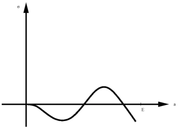
_{, substitute (109) into (106), and linearize to obtain the} characteristic equation

4 3 2

3 2

. r

a Ea a

H

σ= − + − ₍₁₁₀₎ When the film wets the substrate, r>0 and a typical graph of (110) is as shown in Figure 1.

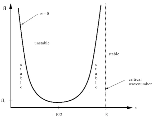
[image:13.595.221.528.480.705.2]

In Figure 2 we plot the neutral stability condition

σ

=0 for the film thick-ness H versus a. We see that there is a critical film thickness, H_c below

(14)

[image:14.595.213.522.64.295.2]

DOI: 10.4236/jamp.2018.64074 877 Journal of Applied Mathematics and Physics Figure 2. Schematic of the stability diagram for the film thickness H versus

perturba-tion wavenumber a.

which every film thickness is stable,

1 3

2 8 c

r H

E

 

=  

  (111)

and there is a critical wave number, ac above which every film thickness is sta-ble,

. c

a =E (112) The evolution equation thus has the property that sufficiently thin films are stabilized by the wetting effect, but thicker films are unstable to the stress driven morphological instability.

6. Summary

We derived a self-contained evolution equation where the film thickness is smaller than wavelength of surface variations. Our evolution equation includes effects of anisotropic elastic constants for cubic symmetry in the film and iso-tropic elastic constants in the substrate, isoiso-tropic surface energy, and wetting energy. This evolution equation possesses steady state solutions corresponding to island formation, and is a possible candidate for use in large scale simulations of island systems.

Acknowledgements

(15)

References

[1] Kastner,M.A. (1996) Mesoscopic Physics with Artificial Atoms. Proceedings of the 23rd International Conference on Physics of Semiconductors, 1, 27.

[2] Chen, M. and Porod, W. (1995) Design of Gate-Confined Quantum-Dot Structures in the Few-Electron Regime. Journal of Applied Physics,78, 1050.

https://doi.org/10.1063/1.360339

[3] Asaro, R.J. and Tiller, W.A. (1972) Interface Morphology Development during Stress Corrosion Cracking: Part I. via Surface Diffusion. Metallurgical and Materials Transactions B, 3, 1789-1796.

https://doi.org/10.1007/BF02642562

[4] Grinfeld, M.A. (1986) Instability of the Interface between a Non-Hydrostatically Stressed Elastic Body and a Melt. Doklady Akademii Nauk SSSR Sov.Phys. Dokl. 31, 831.

[5] Srolovitz,D.J. (1989) On the Stability of Surfaces of Stressed Solids. Acta Metallur-gica,37, 621-625. https://doi.org/10.1016/0001-6160(89)90246-0

[6] Spencer, B.J., Voorhees, P.W. and Davis, S.H. (1991) Morphological Instability in Epitaxially Strained Dislocation-Free Solid Films. Physical Review Letters,67, 3696.

https://doi.org/10.1103/PhysRevLett.67.3696

[7] Daruka, I., Tersoff, J. and Barbasi, A.L. (1999) Shape Transition in Growth of Strained Islands. Physical Review Letters,82, 2753.

[8] Nix, W.D. (1989) Mechanical Properties of Thin Films. Metallurgical and Materials Transactions A,20A, 2217. https://doi.org/10.1007/BF02666659

[9] Gao, H. (1991) Stress Concentration at Slightly Undulating Surfaces. Journal of the Mechanics and Physics of Solids,39, 443-458.

https://doi.org/10.1016/0022-5096(91)90035-M

[10] Gao, H. (1991) A Boundary Perturbation Analysis for Elastic Inclusions and Inter-faces. International Journal of Solids and Structures,28, 703-725.

https://doi.org/10.1016/0020-7683(91)90151-5

[11] Grinfeld, M.A. (1993) The Stress Driven Instability in Elastic Crystals: Mathematical Models and Physical Manifestations. Journal of Nonlinear Science,3, 35-83.

https://doi.org/10.1007/BF02429859

[12] Berrehar, J., Caroli, C., Lapersonne-Meyer, C. and Schott, M. (1992) Surface Pat-terns on Single-Crystal Films under Uniaxial Stress: Experimental Evidence for the Grinfeld Instability. Physical Review B, 46, 13487.

https://doi.org/10.1103/PhysRevB.46.13487

[13] Jesson, D.E., Pennycook, S.J., Baribeau, J.M. and Houghton, D.C. (1993) Direct Im-aging of Surface Cusp Evolution during Strained-Layer Epitaxy and Implications for Strain Relaxation. Physical Review Letters, 71, 1744.

[14] Yang, W.H. and Srolovitz, D.J. (1994) Surface Morphology Evolution in Stressed Solids: Surface Diffusion Controlled Crack Initiation. Journal of the Mechanics and Physics of Solids,42, 1551-1574. https://doi.org/10.1016/0022-5096(94)90087-6 [15] Spencer, B.J. and Meiron, D.I. (1994) Nonlinear Evolution of the Stress Driven

Morphological Instability in a Two Dimensional Semi-Infinite Solid. Acta Metallur-gica et Materialia,37, 621.

(16)

DOI: 10.4236/jamp.2018.64074 879 Journal of Applied Mathematics and Physics Stress-Driven Morphological Instability. Journal of Applied Physics, 91, 9414.

https://doi.org/10.1063/1.1477259

[17] Spencer, B.J. and Tersoff, J. (1996) Equilibrium Shapes of Small Strained Islands. Materials Research Society Symposia Proceedings, 399, 283-288.

https://doi.org/10.1557/PROC-399-283

[18] Spencer, B.J. and Tersoff, J. (1997) Equilibrium Shapes and Properties of Epitaxially Strained Islands. Physical Review Letters, 79, 4858-4861.

[19] Kukta, R.V. and Freund, L.B. (1997) Minimum Energy Configuration of Epitaxial Material Clusters on a Lattice-Mismatched Substrate. Journal of the Mechanics and Physics of Solids,45, 1835-1860.https://doi.org/10.1016/S0022-5096(97)00031-8

[20] Rudin, C.D. and Spencer, B.J. (1999) Equilibrium Island Ridge Arrays in Strained Solid Films. Journal of Applied Physics,86, 5530-5536.

https://doi.org/10.1063/1.371556

[21] Shanahan, L.L. and Spencer, B.J. (2002) Interfaces and Free Boundaries. Interfaces and Free Boundaries,4, 1-25. https://doi.org/10.4171/IFB/50

[22] Tekalign, W.T. and Spencer, B.J. (2007) Thin-Film Evolution Equation for a Strained Solid Film on a Deformable Substrate: Numerical Steady States. Journal of Applied Physics,102, Article ID: 073503. https://doi.org/10.1063/1.2785024

[23] Zhang, Y.W. and Bower, A.F. (1999) Numerical Simulations of Island Formation in a Coherent Strained Epitaxial Thin Film System. Journal of the Mechanics and Physics of Solids, 47, 22730-2297. https://doi.org/10.1016/S0022-5096(99)00026-5

[24] Bergamaschini, R., Salvalaglio, M., Backofen, R., Voigt, A. and Montalenti, F. (2016) Continuum Modelling of Semiconductor Heteroepitaxy: An Applied Perspective. Advances in Physics, 1, 331-367.

[25] Liu, P., Zhang, Y.W. and Lu, C. (2003) Coarsening Kinetics of Heteroepitaxial Isl-ands in Nucleationless Stranski-Krastanov Growth. Physical Review B, 68, Article ID: 035402. https://doi.org/10.1103/physrevb.68.035402

[26] Golovin, A.A., Davis, S.H. and Voorhees, P.W. (2003) Self-Organization of Quan-tum Dots in Epitaxially Strained Solid Films. Physical Review E, 68, Article ID: 056203. https://doi.org/10.1103/PhysRevE.68.056203

[27] Tekalign, W.T. and Spencer, B.J. (2004) Evolution Equation for a Thin Epitaxial Film on a Deformable Substrate. Journal of Applied Physics, 96, 5505-5512.

https://doi.org/10.1063/1.1766084

[28] Pang, Y. and Huang, R. (2006) Nonlinear Effect of Stress and Wetting on Surface Evolution of Epitaxial Thin Films. Physical Review B, 74, Article ID: 075413.

https://doi.org/10.1103/PhysRevB.74.075413

[29] Levine, M.S., Golovin, A.A., Davis, S.H. and Voorhees, P.W. (2007) Self-Assembly of Quantum Dots in a Thin Epitaxial Film Wetting an Elastic Substrate. Physical Review B, 75, Article ID: 205312. https://doi.org/10.1103/PhysRevB.75.205312