A Fuzzy Data Driven Paradigmatic Predictor

A Fuzzy Data-Driven Paradigmatic

Predictor

Farzad Amirjavid∗ Hamidreza Nemati∗∗ Sasan Barak∗∗∗

∗_{Edward S. Rogers, Department of Electrical and Computer} Engineering, University of Toronto, Toronto, Canada (e-mail:

[email protected]).

∗∗_{Engineering Department, Lancaster University, Lancaster, UK} (e-mail: [email protected]).

∗∗∗_{Department of Management Science, Lancaster University} Management School, Lancaster, UK (e-mail: [email protected]).

Abstract: Data-driven prediction of future events is to provide decision-makers Predictive Information (PI) to decrease human-error. They usually desire possession of a predictor which works independently from the humanized configurations and works efficiently and accurately. The accurate data-driven prediction of the systems’ behavior is the primary focus of this paper. We define the future state of a system is a set of uncertain values, which can be modeled by fuzzy numbers. The future machine state is not very dissimilar to the current status, and the next event is a sort of behavior repetition. The PI also justifies the system being in a trend to achieve a goal, and it counts the unplanned contextual reactions of the system. In this paper, we come up with a fuzzy data-driven predictor application to foretell the system behavior.

Keywords:Fuzzy logic, temporal data analytics, adaptive learning, systems theory.

1. INTRODUCTION

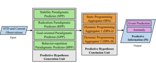
The Predictive Information (PI) is a sort of actionable insight, which allows decision-makers to act upon, and which gives them enough insight into the future that the actions that should be taken become clear. Technically, to provide initial data of system behaviors experts perform the frequent observations on the systems and form the Systematic Temporal Datasets (STDs). Then to machin-ery mining of the systems, we attribute four character-istics to their behavior: stability, radicalism, goal achieve-ment, and behavior repetitions [Djaferis and Schick (2000); Rapoport (1986); Lobry (1973)]. Per each paradigm, there is a predictor, and the aggregator concludes the individ-ual predictions into a totalitarian hypothesis, which is the final prediction of the Fuzzy Data-Driven Predictor (FDDP) as shown in Fig.1. We also consider the role of an Anomaly Recognizer, which compares the realized events with predicted ones to find the anomalies. We argue that in Data-Driven Machine Learning (DDML) and prediction, by improving the clustering rule, we can get more accurate results but in faster time. The reason is that it helps to un-derstand the previous and current states more quickly and more precisely to provide biases for prediction. The other criterion to improve the DDML predictions is attention to the new events and trends that happen after training, and we address this issue by the term “adaptivity.” We concentrate on the prediction of the future states of the real-world systems as the initial problem. This paper is organized as the following. In section (2) we discuss the preliminaries of the current paper and we review some important and relevant works. In section (3), we propose our FDDP model. In the next section, we experiment the

Predictive Hypotheses Conclusion Unit Predictive Hypotheses

Generation Unit Radicalism Paradigmatic

Predictor (RPP) STD and Current

Observations Goal-oriented Paradigmatic Predictor (GPP)

Static Programming Aggregator (SPA)

Predictive Information (PI)

Output Input

Stability Paradigmatic Predictor (SPP)

Behavior-repetition Paradigmatic Predictor (BPP)

Dynamic Programming Aggregator 1 (DPA-I) Dynamic Programming Aggregator 2 (DPA-II)

Event Prediction

Anomaly

Fig. 1. The model of Fuzzy Data-Driven Predictor (FDDP) and Anomaly Recognizer (FDDAR)

proposed model (4) and compare the results with others’, and the functionality of the model with other works. In 5, we perform conslusion and propose suggestions to the interested researchers. Finally, we present the applied ref-erences.

2. PRELIMINARY AND THE RELATED WORKS

data points are congested around and how much the size and proportion of the congestions are. A first solution is to choose a clustering method such as k-means or Fuzzy C-Means (FCM). Due to the segmentation operation with k-means, it finds the centroids rapidly. But, knowing the number of clusters is still a requirement. The fuzzy sub-tractive clustering is a known popular algorithms for the problems in which the experts intend to get tailored cluster sizes and positions from STDs [Kruger et al. (2017)]. This algorithm reviews the data, finds the congested areas and defines the soft cluster boundaries in the neighborhood of the data points that are the farthest to the corresponding centroids. There is also a group of works that focus on clas-sification and data modeling rule to improve the prediction rate. This rule is done in a KD manner. We identified the cited papers in Table 1 out of the recent related works that focused on“Clustering” and“Classification” rules in temporal data mining. These works extended/customized derivations of more known algorithms such as “k-means” and “SVM” to their concerning problems.

According to the presented information in Table 1, and considering that a full data-mining cycle includes both clustering and classification then an ideal approach would predict as accurate as 96.5% × 96% = 92.64% with KD strategy and 95.75% × 94% = 90.005% with DD strategy. These rates are usually taken by more complexity order al-gorithms and the total complexity will be ofO(n2) :O(n4). However, a full cycle of DDML, which works independent of expert configurations with light complexity order (O(x), where x < n2_{) is not proposed. To our best knowledge,} if such cycle be proposed then the average prediction accuracy rate with the recent and relevant works will span around the rate of 90 −93%. The proposed predictors are not generally extensible to predict the STDs of other domains and a full human-independent DDML cycle re-garding the model knowledge (unsupervised) and model-training process (DD) is required.

3. FDDP MODELLING

For data-driven machine learning of the system, the m

features (fi|1 ≤ i ≤ m) are observed. Each feature is

assumed to have totally minimum and maximum values, which means {x|x ∈ fi, x ∈ [0 1],1 ≤ i ≤ m}, and

the FDDP analyzes m-dimensional space. The inputs to the FDDP are the observations (oi,j in equation 1),

which are frequently taken off the system behaviors. The observations matrix isST D, which hasmcolumns and n

rows, whereasm, n >0. Therefore, the current observation will sit on the last row, and it will be the n+ 1th_{row of}

the STD matrix.

ST D= 

 

f1 f2 . . . fm

St₁ O1,1 O1,2 . . . O1,m St₂ O2,1 O2,2 . . . O2,m .

. .

. . .

. . . . ..

. . . S_tn On,1 On,2 . . . On,m





 (1)

In Equation (1), fi is the ithworld feature, Stj is thej th

observation or the observation in time j.

In [Amirjavid et al. (2018)], a derivation of subtractive clustering is proposed, which inputs the STD dataset and the desired similarity degrees between the data points of the clusters (ε). The first output of this algorithm is the list of centroids (matrix C) and the sizes of the clusters

(matrixSz).

The first sort of specific clusters that the FDDP forms is the “machine state”. This a set of continuous observations or a set of sequential rows (sti..j) in STD that are similar to each other with similarity degree ofε. A machine state is a fuzzy concept such as:

˜

s_ti..j ={S_tx|S_tx∈ST D, x∈[i..j]|0≤i≤j≤n,

∃C(k)|∀Stx→ |Stx−C(k)|<1−ε},0≤k≤w

(2)

Based on this concept, we determine the present/current state and the previous state. By present/current state, we mean a subset of machine state that are recently observed. This fuzzy set is defined as the following:

˜

Spresent={x|x∈˜sti..j,|x.time−current time| ≤1−ε} (3) Alike the “current state”, the “previous state” is a sort of machine state that includes all the previous machine states but excludes the recent observations:

˜

Spast={x|x∈˜sti..j, |x.time−current time|< ε} (4) We use the basic concepts mentioned above in design of the paradigmatic predictors.

3.1 Stability Characteristic

The systems are stable, and their behavior is stable over the time. By this statement, we infer that the two contin-uous observations from a system are not very dissimilar to each other, and the system changes the machine states smoothly/slowly. If Sti and Sti+1 are two consecutive observations, then a threshold measure symbolized by ε

defines for the maximum difference between two observa-tion vectors:

Sti−Sti+1

< ε,∀i|0> i, i+ 1≤n, ε >0 (5)

The equation (5) indicates each two consecutive observa-tions are similar to each other. Therefore, ifStiis the latest observed status from the world, then the future upcoming stateSti+1 will be a measure in following constraints:

|Stn| −ε < Stn+1

<|Stn|+ε (6)

According to equation (6), the future event will be a vector similar to the present vector, which means|Stn| ∼=

Stn+1

.

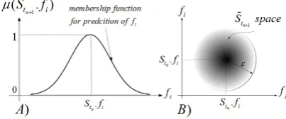
See Figure. 2. In Figure. 2.A, we are presenting that the featureiof the future state of the system will be of Gaus-sian fuzzy number, in which the current value of feature

i has the highest fuzzy membership value to occur in future. In Figure. 2.B, we are presenting a two dimensional presentation of the future state of the features i and j. This space is the product ofstn.fi×stn.fj. This prediction space is a fuzzy set. It gives the highest possibility degree of occurrence to the center of the circular space, which refers to the current value of feature i and the current value of feature j. The εof equation (6) indicates a soft

Table 1. Review of related works that focused on improvement of clustering rule for prediction

KD/DD Approach Accuracy Derived algorithm Complexity Focus

KD

Kim et al. (2016) 85.40% KNN O(n) Classification

Arif et al. (2013) 90.02% ID3 and C4.5 O(n) Classification

Vluymans et al. (2016) 91% FIS O(n.log(n)) Classification

Lopez-Garcia et al. (2016) 83.10% FRBS N/A Classification

Lippi et al. (2013) 95% Regression and SVM O(n) Classification

Baggenstoss and Harrison (2016) 93% SVM N/A Classification

Abercrombie and Friedl (2016) 96.50% HMM O(n2_{) Classification}

KD

Huang et al. (2013) 75% Regression O(n) Clustering

Debonnaire et al. (2016) 87% K-means O(n) Clustering

Wang et al. (2017) 96% Hierarchical O(n2.log(n)) Clustering

DD Yin et al. (2017) 95.75% SVM O(n2) Classification

DD

Mori et al. (2016) 71% K-means O(n) Clustering

Kruger et al. (2017) 90% FCM O(n) Clustering

radius of a circle that represents the possible future values of the featurei. Theεdoes not represent a hard boundary indicating the impossibility measures of the world features, but it shows the limitation implied in current calculations. A possibilistic/fuzzy 2D space as similar as the Figure. 2.B can be drawn per each couple of the features to predict totally the Stn+1 vector. The possibility degrees at the radius borders and beyond there are not zero, but not noticeable. As a result by this we indicate that by exclusive respect to the stability feature of the systems, the vector

Stn+1 is predicted in the form of a multidimensional fuzzy number, which is ˜Stn+1.

Definition 1: Current state.TheCurrent observations cluster is the cluster, which includes the current obser-vation and the last recent obserobser-vations from STD. The algorithm for determination of current state cluster is in Fig. 3. The SPP performs this process. We show fuzzy space of ˜Stn+1, which is produced by SPP, by the notion

˜

PSP P. ByPSP P we point to the defuzzified of the ˜PSP P.

3.2 Radicalism Characteristic

By radicalism, we address the tendency of a dynamic system to leave the current state regardless of whatever reason makes the system leaves the current status. A fuzzy operator called Absolute Fuzzy Symmetrizer Operator (AFSO) finds the most dissimilar status to the current status [Amirjavid (2014); Amirjavid et al. (2018)]:

AF SO(Stn) =S 0

tn ={1−x|x∈Stn.f i,∀i|i∈[1..m]} (7)

By this paradigm, the future state of the system is:

Input STD, ℇ

set CSCL = Null

d = firstRow(STD) insertd inCSCL

c = d

is dist≤ℇ? Yes

set CSCL = Null insertd inCSCL

c = d

output cprevious

No

insertd inCSCL c = centroid(CSCL, ℇ) d = nextRow(STD)

dist = distance(c, d)

Fig. 3. Algorithm regarding Dynamic formation of current state cluster (current fuzzy state)

Stn+1= (AF SO(Stn) +Stn)×λ , 0≤λ≤1 (8) In (8), theλis a factor that indicates the tendency of the system to the radicalism behavior. We show fuzzy space of ˜Stn+1, which is produced by RPP, by the notion ˜PRP P.

3.3 Goal Orientation Characteristic

Systems are to achieve a particular goal. The goal is a world state, and to make it the system transits a series of temporary states. The goal is a fuzzy vector ˜G, which justifies the next state of the system in transition to meet it. Therefore, the future machine state will be in a possibilistic space between theStn and the ˜G:

Stn+1={x˜|x˜∈[Stn,G˜]} (9)

In (9), the ˜Gis not known, but the next machine state is in trend of the two precedent states to achieve the goal:

Stn+1 = (Stn−Stn−1) +Stn= 2Stn−Stn−1 (10) The present state in (10) comes from the algorithm in Fig. 3, and the previous state comes from the algorithm in Fig. 4. The GPP performs the prediction based on goal orientation feature of the systems. We show fuzzy space of ˜Stn+1, which is produced by GPP, by the notion ˜PGP P. ByPGP P we point to the defuzzified of the ˜PGP P.

3.4 Behavior Repetition Paradigm

The systems usually repeat their behaviors. We expect the system repeats a behavior whenever the context (a set of preliminary conditions) for this issue comes up. We define the context as the similar state in STD and the ”behavior repetition” as the following state that the system has already experienced in that situation:

˜

S_tn+1= ˜S_tx+1|S˜_tn∼= ˜S_tx, x∈[1...n−1] (11)

Input STD, ℇ

d = firstRow(STD)

read cas ccurrent dist = distance(ccurrent, d)

is dist≤ ℇ? Yes

cprevious= c

output cprevious No

d = nextRow(STD)

In (11), we are indicating that the future event will be an action that the system has already accomplished whenever it was in similar context.

Theorem 1: According to the stability paradigm in (5, 6) since two consecutive observations are similar, then the BPP output (PBP P) as the future state of the machine is

the most similar centroid in history of the system behavior: ˜

S_tn+1= ˜S_tx|_S˜

tn∼= ˜Stx, x∈[1...n−1] (12) Therefore, according to the (12), the BPP calculates the centroid, which is the most similar centroid to the current observation as the future event. We show fuzzy space of

˜

Stn+1, which is produced by BPP, by the notion ˜PBP P. By

PBP P we point to the defuzzified of the ˜PBP P.

3.5 Aggregation of The Paradigmatic Predictions

We apply an aggregator to achieve a single number as of the final prediction. See Fig. 1. Presuming the “XPP” and “YPP” are two typical paradigmatic predictors, and we define theAggregate(PXP P, PY P P). The predictive values

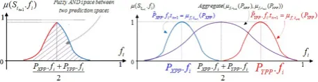
of XPP and YPP are either intersected or distinct/disjoint. In Fig. 5 and Fig. 6 we are providing a visual representa-tion of the intersecrepresenta-tion and distincrepresenta-tion between two fuzzy predictions.

If the centroids of ˜PXP P and ˜PY P P are close to each

other then they make intersection area like in Fig. 5.A and Fig. 6.A. The radius or effective range of centroids are inLmatrix. TheL valuescorrespond the radius measures of the clusters. The predictive centroids make intersection area if:

ABS( ˜PY P P−P˜XP P) ≤ L valuesXP P+L valuesY P P (13) In the case that equation (13) is valid, then the two fuzzy numbers coming from paradigmatic predictors produce intersection areas.

Proposition 1: If the predictors make an intersection area (see Fig. 7.A, Fig. 8.A), then the possible area of the occurrence of the predictive event is a member of the intersection area of two paradigmatic predictors, and the plausible punctual event is at the average (in half distance) of the corresponding centroids.

˜

PF DDP = ˜PXP P∩P˜Y P P, ˜

PF DDP =Average(PXP P, PY P P) =

PXP P+PY P P 2

(14)

If Eq. (13) is not valid, Eq. (14) will not be valid too. The reason is that although, by (13) the plausible event

Fig. 5.1-D intersected (A) and disjoint (B) prediction spaces

Fig. 6.2-D intersected (A) and disjoint (B) prediction spaces

Fig. 7.1-D aggregation of the intersected (A) and disjoint (B) XPP and YPP

Fig. 8.2-D aggregation of the intersected (A) and disjoint (B) XPP and YPP

is in space between the predictors, the equation (14) recommends contradictorily low impossibility degree for this estimation. To resolve this problem, the FDDP creates a third larger cluster, which includes, both of the clusters as the predictive estimation. See Fig. 7.B, Fig. 8.B.

Proposition 2: The aggregated prediction of disjoint paradigmatic predictions are computed by (14). This is the new centroid of the new auxiliary cluster. The radius of the new cluster is (R):

R = L values + distance( ˜PY P P, ˜ PXP P) 2

= L values + ABS( ˜PY P P− ˜ PXP P) 2

(15)

In Fig. 8.B, we show the auxiliary cluster formed by two disjointed fuzzy numbers. The position of the new centroid is calculated by (14), but the new radius of the new cluster (R) is:

R = L values + distance( ˜PY P P, ˜ PXP P) 2

= L values + ABS( ˜PY P P− ˜ PXP P) 2

(16)

The R of (16) is demonstrated in Figure. 8.B. The final prediction of the FDDP is a fuzzy space represented by the symbol ˜PF DDP, and the plausible measure isPF DDP,

which is the defuzzified of ˜PF DDP.

Proposition 3: We define the “Problem Solution Space (PSS)” is the auxiliary cluster, which includes all the individual clusters formed by paradigmatic predictors. “R” from equation (16,15) is the radius of this cluster, and the position of the center of this cluster is:

P os(P SS) =Average(P os(SP P), P os(RP P), P os(GP P), P os(BP P)) (17) The PSS indicates that the FDDP expects that the predic-tive values are in PSS and we consider it to beimpossible that the event occurs out of the PSS specs.

Theorem 2:The “Static Programming Aggregation (SPA)” function inputs the predictive values in type of the fuzzy numbers from individual paradigmatic predictors and re-turns the aggregated predictive value by:

[P SS,P˜F DDP] =SP A( ˜PSP P,P˜RP P,P˜GP P,P˜BP P) =π.R2, Average(PSP P, PRP P, PGP P, PBP P)

(18)

cer-Fig. 9. By dynamic programming the plausible hypotheti-cal prediction moves from average/center toward the more precise predictor (YPP), while the PSS does not change.

tain/reliable predictions regarding the UOS behavior in comparison to bigger values of “R”.

3.6 Dynamic programming Aggregation (DPA)

In equation (18), we presume all the paradigmatic predic-tors have equal weights in the SPA aggregation process. However, in reality, one or more paradigmatic predictors usually work more accurately than the otherstemporarily or permanently. To adjust the weight of the paradigmatic predictors in aggregation process FDDP evaluates the functionality of the individual predictors:

P rediction Accuracy of XP P =|PXP P,n−Stn| (19) In (19), the XPP is a typical paradigmatic predictor:

XP P = {x|x ∈ {SP P, RP P, GP P, BP P}}. Stn is the current observation,PXP P,nis the prediction ofXP P; the

concerning process is done in time n−1 (previous time) and supposed to be observed in timen(current time).

Dynamic Programming Aggregation type 1 (DPA-I): Presuming XP Pi, i = 1..4 predicts more accurately

than others in time n (current time), then it will have additional weight in average making rule 14 to predict the

Stn+1:

PF DDP =Average(PXP Pi, PXP Pi, PXP Pk)| k= 1..4, k6=i (20) In DPA-I method, the temporarily effect of the “more accurate” predictor is taken into account and at the next observation FDDP redoes the processes in equations (19, 20).

Dynamic Programming Aggregation type 2 (DPA-II):This reflects the permanent effect of the predictors in prediction accuracy. DPA-II counts the number of times each of the XPPs are the most accurate in precision since the beginning to the current time:

PF DDP =

(iSP P.PSP P) + (iRP P.PRP P) + (iGP P.PGP P) + (iBP P.PBP P)

iSP P+iRP P+iGP P+iBP P

,

iXP P≥0, iXP P ∈N

(21) The visual presentation of the effect of dynamic program-ming is in Fig. 9. The objective of dynamic programprogram-ming is to drive the predictions to the more accurate predictors while the PSS does not increase. In this way, the certainty of the predictions (“R” values) does not decrease but the accuracy of the predictions might increase.

4. EXPERIMENTING THE FDDP

We experimented the functionality of the FDDP on the monthly Fama-French 3-Factor Model Dataset.This data is an indicator of the systematic risk of an investment aris-ing from exposure to general market movements. The FF 3-factor model dataset includes three parameters, which

are (rm−rf),SM B andHM L. We predicted the data of

FF three parameters model since July 1926 to November 2016. The first step to deal with this dataset is to normalize the dataset so that the data of fi in STD. We examined

the FDDP with multiple values ofε(an indicator of cluster size) for values between zero and one. In overal, the SPA predicts most accurately at ε = 0.15. In Fig. 10, we are representing the inaccuracy rates of the paradigmatic predictors as well as the aggregators atε= 0.15. According to our test results, in average the static programming aggregation gives the best outcome; however, the dynamic method improves the maximum amount of prediction in-accuracy. See Table 2.

The main objective to accomplish this experiment is to

Table 2. Dynamic programming aggregation of the FF data inε= 0.15

Inaccuracy DPA-Il DPA-II

Average 0.02591598 0.026053

Minimum 0.000894579 0.001572

Maximum 0.215938889 0.218264

show the functionality of the clustering rule within the paradigmatic predictors. We also reflected the applica-tion of fuzzy logic in aggregaapplica-tion of predicapplica-tions that led to more reliable accuracy rates. Moreover, the adoptive learning technique improved the results. Statistically, the BPP predicted 25.6931608% of the observations more ac-curate than the others, then SPP by 25.23105366%, RPP by 24.7689464% and GPP by 24.1219963% predicted the more accurate the FF data, which explains the character-istic of the FF dataset. According to the related works in section (2), the other proposed methods are customized to and dependent on the problem context. In average they do not propose an accuracy rate any better than 96%. Especially, if we desire a data-driven approach that works fast (being ofO(n)), then the expected accuracy rate drops to less than 71−90% [Yang et al. (2015); Mori et al. (2016)]. Since, regression lets us model and predict the datasets with no expert prejudgment, then we selected the linear regression method to compare our works with it. To compare the FDDP results on FF dataset with the regression results, we set a linear regression model to learn each data column by the other columns. For example, column 1 learns the columns 2 and 3, and the column 2 learns the column 3. The average RSQ rate of the linear regression on FF data is 0.229701927, which indicates the

SPP RPP GPP BPP SPA DPA-I DPA-II 0

0.05 0.1 0.15 0.2 0.25 0.3 0.35 0.4

0.03129

0.03129 0.31306

0.02765 0.00177 0.24813

0.02796 0.00123 0.250867

0.02489 0.00140 0.153433

0.02602 0.00156 0.21368

0.02591 0.00089 0.21593

0.02605 0.00157 0.21826

Fig. 10. Inaccuracy rates in prediction of FF dataset at

inaccuracy rate at the learning step. Therefore, at the prediction time the average inaccuracy rate for prediction is expected to be worse. The FDDP with DPA-II method achieved the inaccuracy rate of 0.026053 at the predic-tion time. This is though the FDDP works with no pre-configuration and training data, but the regression model is trained with full FF data. [Arif et al. (2013)] for classifi-cation of the same dataset. The RSQ rate (inaccuracy rate at the learning step) for the Kagaru Airborne Dataset is 3.064886%, while the FDDP achieved the rate of 1.3112% for prediction inaccuracy of that dataset.

5. CONCLUSION

Four paradigms in the interpretation of systematic tem-poral data series are considered to predict future events. The FDDP explains the behavior of a system regarding its predictability proportion with the paradigmatic predic-tors. For instance, since GPP and RPP predicted the FF data the most accurate then we resemble the FF dataset as a radical and goal oriented dataset. We experimented the FDDP on FF dataset to survey the accuracy of pre-diction, and we verified the role of dynamic programming to propose inaccurate average predictions. We recommend the future researchers to expand the paradigmatic pre-dictors. In particular, we suggest adding the probabilistic predictors in the box of paradigmatic predictors and study their role if it could improve the prediction specs such as accuracy rate and the reliability factor. We propose also to survey the proposed model to recognize the anomalies in economical systems so that the systematic economical crises could be inferred before their occurrence.

ACKNOWLEDGEMENTS

The first author is profoundly thankful and highly in-fluenced by the works of professor Kostas N. Platan-iotis ([email protected]), and Dr. Arash Moham-madi ([email protected]). The second au-thor’s work is supported by the Engineering and Phys-ical Sciences Research Council (EPSRC), grant number EP/R02572X/1, and the National Centre for Nuclear Robotics (NCNR). The third author is supported by the Czech Science Foundation (GACR Project GA 17-22662S) and Operational Program Education for Competitiveness - Project No. CZ.1.07/2.3.00/20.0296.

REFERENCES

Abercrombie, S. and Friedl, M. (2016). Improving the consistency of multitemporal land cover maps using a hidden markov model.IEEE Trans. Geosci. Rem. Sens., 54, 703–713.

Amirjavid, F. (2014). A fuzzy temporal data-mining model for activity recognition in smart homes. PhD Dissertation, University of Quebec in Chicoutimi. Amirjavid, F., Spachos, P., and Plataniotis, K. (2018). 3-d

object localization in smart homes: a distributed sensor and video mining approach. IEEE Systems Journal, 12, 1307–1316.

Arif, F., Suryana, N., and Hussin, B. (2013). A data mining approach for developing quality prediction model in multi-stage manufacturing. Int. J. Computer Appli., 69, 35–40.

Baggenstoss, P. and Harrison, B. (2016). Class-specific model mixtures for the classification of acoustic time series. IEEE Trans. Aero. Elect. Sys., 52, 1937–1952. Debonnaire, N., Stumpf, A., and Puissant, A. (2016).

Spatio-temporal clustering and active learning for change classification in satellite image time series.IEEE J. Selected Topics in Appl. Earth Observ. Rem. Sens., 9, 3642–3650.

Djaferis, T. and Schick, I. (2000). System Theory: Model-ing, Analysis and Control. Springer, New York. Huang, B.W., Wang, K.W., Wei, L.Y., and Peng, W.C.

(2013). A hybrid prediction algorithm for traffic speed prediction. Adv. Intell. Syst. Appl., 1, 281–296.

Kim, J., Han, Y., and Lee, J. (2016). Data imbalance problem solving for smote based oversampling: Study on fault detection prediction model in semiconductor manufacturing process. ITCS 2016, 79–84.

Kruger, B., Vogele, A., Willig, T., Yao, A., Klein, R., and Weber, A. (2017). Efficient unsupervised temporal segmentation of motion data.IEEE Trans. Multimedia, 19, 797–812.

Lippi, M., Bertini, M., and Frasconi, P. (2013). Short-term traffic flow forecasting: an experimental comparison of time-series analysis and supervised learning. IEEE Trans. Intell. Transport. Syst., 14, 871–882.

Lobry, C. (1973). Dynamical Polysystems and Control Theory. Springer, Dordrecht.

Lopez-Garcia, P., Osaba, E., Onieva, E., Masegosa, A., and Perallos, A. (2016). Short-term traffic congestion forecasting using hybrid metaheuristics and rule-based methods: A comparative study. 17th CAEPIA 2016, Salamanca, Spain, 290–299.

Lu, M., Lai, C., Ye, T., Liang, J., and Yuan, X. (2017). Vi-sual analysis of multiple route choices based on general gps trajectories. IEEE Trans. Big Data, 3, 234–237. Mori, U., Mendiburu, A., and Lozano, J. (2016). Similarity

measure selection for clustering time series databases. IEEE Trans. Knowl. Data Engin., 28, 181–195.

Rapoport, A. (1986). General System Theory: Essential Concepts & Applications. Routledge, Cambridge. Vluymans, S., Tarrago, D., Saeys, Y., Cornelis, C., and

Herrera, F. (2016). Fuzzy multi-instance classifiers. IEEE Trans. Fuzzy Syst., 24, 1395–1409.

Wang, L., Zhao, X., Si, Y., Cao, L., and Liu, Y. (2017). Context-associative hierarchical memory model for hu-man activity recognition and prediction. IEEE Trans. Multim., 19, 646–659.

Yang, L., Wang, J., and Khuhro, M. (2015). Pippy search: Anomaly traffic clustering. IEEE Int. Conf. Smart City/SocialCom/SustainCom (SmartCity), Chengdu, 378–383.