Predict Edges in Fliker Social Network Using Data Mining Method

(1)

Predict Edges in Fliker Social Network Using

Data Mining Method

Amir Hossein Rasekh1, Zeinab Liaghat2, Ala Mahdavi3

1_{Young Researchers Club, Shiraz Branch, Islamic Azad University, Shiraz, Iran} 2_{Young Researchers Club, Sepidan Branch, Islamic Azad University, Sepidan, Iran}

3_{Sharif University of Technology, Tehran, Iran}

Email: {ahrasekh, zliaghat2010}@gmail.com, [email protected]

Received January 4, 2012; revised March 18, 2012; accepted March 26, 2012

ABSTRACT

Using social networking services is becoming more popular day by day. The websites of the social networks like face-book currently are among the most popular internet services just after giant portals such as Yahoo, MSN and search engines like Google. One of the main problems in analyzing these networks is the prediction of relationships between people in the network. The purpose of this paper is to forecast the friendship of a person with a new person using exist-ing data on Flickr website accurately. In this paper, we achieved about 90% percent correct prediction with regards to the results which are obtained by using data mining methods.

Keywords: Social Network; Data Mining; Link Prediction; Regression

1. Introduction

A social network is a social structure consists of personal or organizational groups. These groups are connected to each other by one or some dependencies [1].

1.1. History of Social Networks

Cyberspace provides the possibility of the formation of new societies for users. All philosophers of social and cultural sciences have mentioned “being face-to-face”, “number limitation”, and “being based on emotional relationships but not rational” as fundamental features of the society.

For the first time, in 1960, the subject of social networks was proposed in Illinois University of the United States of America. After that the first social network website was set up to the internet address “Six Degrees. com”. But after year 2002, business explosion in websites of social networks such as LinkedIn, Orkut, and etc made a great evolution in this area and prospered social networking.

In 2004, Friendster and MySpace social networking websites hold top spots with 7 and 4 millions of users respectively. In the same year Facebook website was launched.

The year of emerging rules for social networks was 2005 when a large amount of people’s personal information was in hands of these networks. Therefore, specific rules for keeping the information secret and types of re-

lationships were regulated. Eventually year 2006, was the year of rapid increase of users and visitors of social networks.

1.2. Development of Social Networks in the World

In April 2008, Facebook introduced its main web pages in different languages which propelled the site to 153 percent growth relative to past year.

Today, the popularity of social networks among people is undeniable. These social networks provide users with a lot of facilities for interpersonal communications. The networks are instantaneously growing by joining new individuals or by creation of a new connection between existing ones in the network. One of the major problems in analyzing these types of networks is the prediction of relationships between individuals within the network [2].

Link prediction is a subfield of analyzing social networks in which one should deduces or estimates a series of links that are not directly observable or do not exist with regards to existing observations and links.

Generally, forecasting relationships includes the following fields.

1) Link forecasting existence. That is to predict whe- ther exist a connection between two arbitrary nodes.

(2)

3) Regression of relations.

2. Research Literature Review

Although most primary studies on social networks are done by social sciences scholars and the psychologists, numerous efforts by computer scientists are performed recently [3]. Nowadays most works are focused on stu- dying and analyzing social networks graphs. Many efforts have carried out to solve the problem of exclusive prediction of social networks [4,5].

One of the other works done by Faloutsos et al. is in- troducing an item called sub-graph link. A small sub- graph is the best link in a social network. They also proposed an effective algorithm based on electronic rules which finds sub-graphs connections in large social networks. Number of sub-graphs could be used in computa- tion of various values for solving the prediction problem of social networks, especially when the networks are very large [6].

Mr. Cranshaw et al. have presented a method in mobile social networking, manner in which it spoke of the relationship between the numbers of mobile users in the physical world to discover social networks [7].

In recent study researchers supervised methods are used to link prediction. Mr. Lichtenwalter et al. detailed the challenges that a link exists in the prediction system were analyzed. In this paper discussing imbalance problems and proposing to treat prediction separately for different classes of potential friends [8].

3. Research Motivation and Data

The purpose of this paper is to predict friendship relationship with high probability. This prediction helps social network websites a lot in finding out the existence of a relation between two individuals. To do so we used the data of Kaggle competition site which have been collected from Fliker social site [9]. Fliker is a huge social network having 36 millions of users and 35 billions of photos. This site is full of friendship data, including people’s comments, group memberships, friend suggestions, clicking on favorite’s photo, and restricting the visit to some of the friends and families.

Data consist of two test and train files which we analyzed them separately in the following.

The first file, “Social_Train.zip”, contains of 7,237,983 records with two columns of first person and second per-son in Figure 1. These columns are filled numerically

which denotes person unique number that assigned to a person within the whole data. There are 1,133,574 different individuals in the data. Each column shows that the first person is friend with the second person.

The second file is “Social_Test.zip” which includes 8960 records and three columns, like the first file, it has

two columns of first and second person, and the third column is the prediction column which represents whe- ther or not the first person and the second person are friends in Figure 2. These columns are filled with 0 and

1, value 1 in the case of friendship existence, and value 0 otherwise. These data have been collected from Decem-ber 2010 to January 2011.

4. The Proposed Method

In this paper, we exploited ROC curve to compute the validity of predicted values. ROC is a strong simulation tool which is used in medical decision making, psycho- logy, communications, and whenever need for threshold values is concerned [10].

In the beginning, for recognizing the type of data and the circumstances of ROC rating, we generated a series of data and obtained results as we mention here.

Firstly the prediction column is loaded with a series of random numbers between 0 and 1. ROC was obtained about 0.435 using these numbers. Then in the second step, we filled half of the prediction columns of the test file with one, and the other half with zero, which resulted in ROC of about 0.46. In the third step, we filled all the data with zeros and after submitting it, ROC was obtained equal to 0.5. In step four, all data of prediction columns were filled with ones, and again ROC = 0.5 was obtained after submission. With regards to the last two steps, it can be concluded that the number of one’s or zeros, i.e. having friendship relation between two individuals, are equal in the whole test data.

[image:2.595.367.476.499.605.2]

The other studied work was that it’s probable to get better ROC, by swapping predicted value (zero to one, and one to zero) in the prediction column not having

Figure 1. Train a sample of data.

(3)

good ROC. We assumed one of earlier predictions in which ROC was obtained 0.468, and with regards to new assumptions /theories we predict that ROC result will be improved by inversing data. So by submitting the in- verted data, ROC result increased to 0.532 which this result supports our hypothesis. This result in ROC represents that the two predicted columns are complements, and the sum of two ROCs equals one. Considering the above contents we can say that of the 8690 test data, 4345 data are 1, and there exist 4345 data with zero value.

Then in continue, we presumed that “Friend A” represents column one, “Frined B” represents column two, and prediction result of relationship between Friend1 and Friend 2 forms the third column, and we know that train- ing data of the first and the second column certainly related to each other.

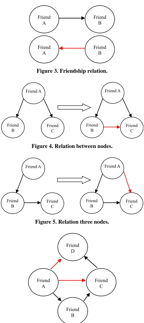
Up to this point we have gathered some information about type of data and their way of implementation, as we mentioned above. In the following we present a few models which could be helpful in identification relationship between two individuals. In the learning data, Friend A is related with Friend B, so it could be forecast that Friend B has relationship with Friend1 as demonstrated in Figure 3. Exploring in learning test data, we recog-

nized that about 400 numbers of data exist in the test data which satisfy this condition.

Another method we used in forecasting links is based on the following principle.

If there is a relationship between paired nodes (a,b) and (a,c), and also there exists a link between them, then the probability of existence of a relationship between nodes (b,c) in future is very high. This is depicted in the

Figure 4 below.

With the assumption that if the paired nodes (a,b) and (a,c) are related and there exists a link between them, then nodes (b,c) are related as well. This means that Friend 1 has relationship with Friend B, and Frined C has relationship with Friend A, so one can conclude that it is probable that Friend B has relationship with Friend A, too. Using this method ROC result was obtained 0.43.

In the next model we actually find a route which includes only three nodes, and then we surmise that the starting point and ending point has direct relationship with each other. As demonstrated in Figure 5, if links

(a,b) and (b,c) exist, then we create the link (a,c) as well. That is, Friend1 has connection with Friend 2, and Frined 2 has connection with Friend 3, so it could be said that it is likely that Friend 1 and Friend 3 have relationship. With this method ROC result was 0.495.

With Regards to Figure 6 in the followed step, sup-

posing the relationships between paired nodes (a,b), (b,c), and (c,d) , then it is highly probable that a connection exists between paired nodes (a,d) and (a,c). Using this

Friend A

Friend B

Friend A

[image:3.595.308.538.77.590.2]

Friend B

Figure 3. Friendship relation.

Friend A

Friend

B Friend C

Friend A

Friend

B Friend C

Figure 4. Relation between nodes.

Friend A

Friend

B Friend C

Friend A

Friend

B Friend C

Figure 5. Relation three nodes.

Friend A

Friend B

Friend C Friend

D

Figure 6. Relation a node with other nodes.

method we get 0.524 for ROC result.

In the next step, we considered the all methods we had realized, and we put the all relations we predicted, all ones, together and as a consequence we recorded the final ROC which obtained 0.78.

Using Regression for Data Prediction

(4)

In Statistics, such works are realized by different regression methods, and results will be analyzed. In regression Response Variable is estimated by using independent variables, and this variable is the main objective of the most researches [11].

As described earlier, regression methods are applied based on type of the factors in studies. Logistic regression is a particular type of regression which is used in cases that response variable is double-choice or multiple- choice; that is only two or a few different states exist for response variable. This case is often used in medical and sociological research [12,13].

Whenever we want to specify a relationship within a collection of X’s with a dependent variable Y, we are confronting a multivariate problem. In analyzing such problems different mathematical methods are exploited. Logistic regression is a mathematical model which could be used for describing relationship between a number of variables X’s and a two-state or multi-state dependent variable as Y, naming two-state variable is a variable that have just two answers like dying or surviving, being present or absent, and having relationship or not having relationship [14]. Often binary codes are used for such variables. Code “1” is used for positive state (success) if that feature, and code “zero”, for negative state (failure) in Figure 7.

The essential subject in regression topic is finding a relation between response variable Y, and a set of predictor variables such as X1, X2, ··· and Xk. Actually

re-gression technique is seeking to make a relationship like

Y = f(X1, X2, ···, Xk) between observations of Y and ob-servation of X1, X2, ···, Xk. The simplest solution that

one could imagine is the following linear equation.

Y = α + β1X1 + ··· (1) where β0, coefficients are usually estimated by using one sample and with the aid of an estimation method like MMSE1_{method. Although this requires applying some} conditions on response and predictor variables. For ex-ample, presumptions of model linearity, observations independency, normality of response variable distribu-tion, and stability of response variable variance must be hold. As could be considered, because of these condi-tions the linear model is not always effective, and for dif-ferent data proper models should be used.

Sometimes, response variable is a two-state variable. On the other hand, predictor variables that their effect on response variable could be evaluated are quantitative. In this case, it is not possible to use linear model in (1), because left hand side of Equation (1) arbitrates only values 0, and 1, whilst the right hand side could theoretically has any values form –∞ to +∞. Logical regression is a proper solution for these kinds of situations. In this me-

thod, the left-hand side of the equality is converted to a quantitative variable. This is carried out in three steps.

1) Substituting Y with the term Pr[Y = 1] in Equation (1). Apparently, this probability could have any value between 0 and 1.

2) Instead of using direct probability (Pr), its equiva-lent concept, “Odds Ratio” is used. Note that probability

p = 0.9 could be expressed in form of 9 to 1, or OR =

p/p–1 = 0.9/0.1 = 9. It’s obvious that if p = 0 then OR-0, and if p = 0.5 then OR equals one.

3) Deriving the natural logarithm from new response variable OR in order to range of new response variable varies from

–

∞ to +∞. In fact, ln(0) =

–

∞, ln(1) = 0, and ln(+∞) = +∞. It worth to mention that ln(p/1

–

p) is ab- stractly called logit(p). In this case the new model given by:

0 1 1 2 2

[ 1] logit

1 [ 1]

r

k k r

p Y

x x x

p Y    



 

    

 _ _ 

   (2)

To estimate coefficients in (2), a random sample of long “n” is selected, and for those values of response variable and predictor variables are evaluated.

Hence for the sum of n observations of predictor vari-able, there exist J different patterns (j = 1, 2, ···, J) so that for the j’th pattern of predictor variables, there are mj number of observations, and the probability that j’th pattern contains Y = 1 equals:

1 1 2 2

π 1

j j k kj

x x x

j x x x

e e                   

 (3)

Thus the logarithm of coefficients’ likelihood function



0, , ,1 k



     is given by,

 

  

 



1

ln J ln π ln 1 π

j

L  L  yj j mj yj



 



   j (4)

[image:4.595.313.534.570.719.2]

In which yj denotes sum of observations for the j’th pattern. To find the maximum likelihood that obtained by maximization of equity (4) with respect to β, we should solve the following equations, involves k + 1 equation,

Figure 7. Logistic regression plot (Adopted from [4]).

(5)

and k + 1 variable, with respect to β:





1

0

π

J

j

xji yi mj j



 



(5)

The Equations (5) are nonlinear with respect to 0, , ,1 k

    , therefore iterative numerical methods are used to solve them.

In the last step, we obtained ROC = 0.78 for all of pre-viously predicted models. We used Binary Logistic Re-gression for unpredictable states, and the ones we could not able to make an assumption, for which we obtained ROC = 0.89.

5. Experimental Results

With regards to the obtained results in Figure 8 and Table 1;it could be concluded that appropriate model for

predic-tion of one and zero values is to apply logistic regression model on obtained data of previous assumptions.

Table 1. Result summary.

ROC DESCRIPTION

0.435 Generate numbers randomly between 0 and 1

0.46 First half of the test data is filled with one, and the other _{half is filled with zero}

0.5 All data are filled with 0

0.5 All data are filled with 1

0.43 With the assumption that if there exists a link between _{(a,b) and (a,c) nodes, then (b,c) nodes are connected}

0.495 That is if (a,c) and (b,c) exist, then there is a relationship _{between nodes (a,c)}

0.524

If there are relationships between pair nodes (a,b), (b,c), and (c,d) then a relationship exists between two pair nodes (a,d) and (a,c)

0.78 Considering all previous implemented models

0.89 Combination of all previous models along with binary _{logistic regression}

Figure 8. Diagram of studied data.

6. Conclusion

In this paper we exploited various methods for data pre-diction which the best result was to combine all of possi-ble assumptions and relationships along with using logis-tic regression model. From total number of 8690 data, we have correctly predicted about 90% of data, and this model gives us the best result for prediction of zeros and ones value.

7. Future Works

With regards to obtained data from aggregation of pre- viously presented models, and considering number of ones and conclusion yielded from playing with numbers, the number of forecasted ones is more than expected in friendship relationship. To resolve this one may put weights to presented models in a way that the more likely the model is correct, the more it is weight is assigned, and eventually sum of all represents the correct prediction probability of friendship relation.

Z



Result of model X: Z = weight of X * result of model X.

REFERENCES

[1] A. H. Rasekh and Z. Liaghat, “Predictive Relationship of Friendship in Social Networks,” The 5th 2011 Interna- tional Conference on Data Mining,14-15 December 2011, pp. 47-53.

[2] Bruce Hoppe and Claire Reinelt, “Social Network Analy- sis and the Evaluation of Leadership Networks,” The Leadership Quarterly, Vol. 21, No. 4, 2010, pp. 600-619. [3] B. Hoppe and C. Reinelt, “Social Network Analysis and the

Evaluation of Leadership Networks,” The Leadership Quar- terly, Vol. 21, No. 4, 2010, pp. 600-619.

doi:10.1016/j.leaqua.2010.06.004

[4] D. M. Boyd and N. B. Ellison, “Social Network Sites: Definition, History and Scholarship,” Journal of Com- puter-Mediated Communication, Vol. 13, No. 1, 2008, pp. 210-230.

[5] M. Safaei, M. Sahan and M. Ilkan, “Social Graph Genera- tion & Forecasting Using Social Network Mining,”33rd Annual IEEE International Computer Software and Appli- cations Conference, Seattle, 22-24 July 2009, pp. 31-35. doi:10.1109/COMPSAC.2009.110

[6] H. Witten and E. Frank, “Data Mining,” Morgan Kauf-mann Publishers,San Francisco, 2005.

[7] C. Faloutsos, K. McCurley and A. Tomkins, “Fast Discovery of Connection Subgraphs,” International Conference on Knowledge Discovery and Data Mining, New York, 22-25 August 2004, pp. 118-127. doi:10.1145/1014052.1014068 [8] J. Cranshaw, E. Toch, J. Hong, A. Kittur and N. Sadeh,

“Bridging the Gap Between Physical Location and Online Social Networks,” Proceedings of UBICOMP’10, New York, 26-29 September 2010, pp. 119-128.

(6)

http://www.kaggle.com/socialNetwork, 2011.

[10] K. H. Zou, A. James, O. Malley and L. Mauri, “Receiver- Operating Characteristic Analysis for Evaluating Diagnostic Tests and Predictive Models,” Circulation Journal of the American Heart Association, Vol. 115, No. 15, 6 February 2007, pp. 654-657.

[11] D. W. Hosmer and S. Lemeshow, “Applied Logistic Regres- sion,” 2nd Edition, Wiley-Interscience, 2000.

[12] Y. Wang, “A Multinomial Logistic Regression Modeling Approach for Anomaly Intrusion Detection,” Computer &

Security, Vol. 24, No. 8, 2005, pp. 662-647.

[13] J. Zhang, R. Jin, Y. Yang and A. G. Hauptmann, “Modified Logistic Regression: An Approximation to SVM and It Is Applications in Large-Scale Text Categorization,” Procee- dings of the 20th International Conference on Machine Learning, Washington, 21-24 August 2003, pp. 888-895. [14] D. G. Kleinbaum, M. Klein and E. R. Pryor, “Logistic Regre-