Approximate Factoring for A* Search

Approximate Factoring for A

Search

Aria Haghighi, John DeNero, Dan Klein

Computer Science Division University of California Berkeley

{aria42, denero, klein}@cs.berkeley.edu

Abstract

We present a novel method for creating A∗ esti-mates for structured search problems. In our ap-proach, we project a complex model onto multiple simpler models for which exact inference is effi-cient. We use an optimization framework to es-timate parameters for these projections in a way which bounds the true costs. Similar to Klein and Manning (2003), we then combine completion es-timates from the simpler models to guide search in the original complex model. We apply our ap-proach to bitext parsing and lexicalized parsing, demonstrating its effectiveness in these domains.

1 Introduction

Inference tasks in NLP often involve searching for an optimal output from a large set of structured out-puts. For many complex models, selecting the high-est scoring output for a given observation is slow or even intractable. One general technique to increase efficiency while preserving optimality is A∗ search (Hart et al., 1968); however, successfully using A∗ search is challenging in practice. The design of ad-missible (or nearly adad-missible) heuristics which are both effective (close to actual completion costs) and also efficient to compute is a difficult, open prob-lem in most domains. As a result, most work on search has focused on non-optimal methods, such as beam search or pruning based on approximate models (Collins, 1999), though in certain cases ad-missible heuristics are known (Och and Ney, 2000; Zhang and Gildea, 2006). For example, Klein and Manning (2003) show a class of projection-based A∗ estimates, but their application is limited to models which have a very restrictive kind of score decom-position. In this work, we broaden their projection-based technique to give A∗ estimates for models which do not factor in this restricted way.

Like Klein and Manning (2003), we focus on search problems where there are multiple projec-tions or “views” of the structure, for example lexical parsing, in which trees can be projected onto either their CFG backbone or their lexical attachments. We use general optimization techniques (Boyd and Van-denberghe, 2005) to approximately factor a model over these projections. Solutions to the projected problems yield heuristics for the original model. This approach is flexible, providing either admissi-ble or nearly admissiadmissi-ble heuristics, depending on the details of the optimization problem solved. Further-more, our approach allows a modeler explicit control over the trade-off between the tightness of a heuris-tic and its degree of inadmissibility (if any). We de-scribe our technique in general and then apply it to two concrete NLP search tasks: bitext parsing and lexicalized monolingual parsing.

2 General Approach

Many inference problems in NLP can be solved with agenda-based methods, in which we incremen-tally build hypotheses for larger items by combining smaller ones with some local configurational struc-ture. We can formalize such tasks as graph search problems, where states encapsulate partial hypothe-ses and edges combine or extend them locally.1 _For

example, in HMM decoding, the states are anchored labels, e.g. VBD[5], and edges correspond to hidden transitions, e.g. VBD[5]→DT[6].

The search problem is to find a minimal cost path from the start state to a goal state, where the path cost is the sum of the costs of the edges in the path.

1

In most complex tasks, we will in fact have a hypergraph, but the extension is trivial and not worth the added notation.

!_a a!

" →

!_b

b!

"

!_b

a!

" →

!_c

b!

"

1

!_a

a!

" →

! _b

b!

"

!_b

b!

" →

!_c

c!

"

1

!_a

a!

" →

! _b

b!

"

!_a

b!

" →

!_b

c!

"

1

!_a

a!

" →

!_b

b!

"

!_a

b!

" →

!_b

c!

"

1

Local Configurations a' → b' b' → c'

a → b

b → c

3.0 4.0 3.0 2.0

2.0 1.0

2.0 1.0

Factored Cost Matrix Original Cost Matrix 3.0 4.0

3.0 2.0 a → b

b → c

a' → b' b' → c'

c(a → b)

c(b → c)

c(a' → b')c(a' → b')

3.0 4.0 3.0 2.0

2.0 1.0

2.0 1.0

Factored Cost Matrix Original Cost Matrix

3.0 5.0 3.0 2.0

a → b

b → c

a' → b' b' → c'

c(a → b)

c(b → c)

c(a' → b')c(a' → b')

(a) (b) (c)

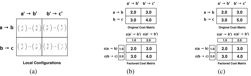
Figure 1: Example cost factoring: In (a), each cell of the matrix is a local configuration composed of two projections (the row and column of the cell). In (b), the top matrix is an example cost matrix, which specifies the cost of each local configuration. The bottom matrix represents our factored estimates, where each entry is the sum of configuration projections. For this example, the actual cost matrix can be decomposed exactly into two projections. In (c), the top cost matrix cannot be exactly decomposed along two dimensions. Our factored cost matrix has the property that each factored cost estimate is below the actual configuration cost. Although our factorization is no longer tight, it still can be used to produce an admissible heuristic.

For probabilistic inference problems, the cost of an edge is typically a negative log probability which de-pends only on some local configuration type. For instance, in PCFG parsing, the (hyper)edges refer-ence anchored spans X[i, j], but the edge costs de-pend only on the local rule typeX →Y Z. We will useato refer to a local configuration and use c(a)

to refer to its cost. Because edge costs are sensi-tive only to local configurations, the cost of a path isP

ac(a). A∗search requires a heuristic function, which is an estimateh(s)of the completion cost, the cost of a best path from statesto a goal.

In this work, following Klein and Manning (2003), we consider problems with projections or “views,” which define mappings to simpler state and configuration spaces. For instance, suppose that we are using an HMM to jointly model part-of-speech (POS) and named-entity-recognition (NER) tagging. There might be one projection onto the NER com-ponent and another onto the POS comcom-ponent. For-mally, a projection π is a mapping from states to some coarser domain. A state projection induces projections of edges and of the entire graphπ(G).

We are particularly interested in search problems with multiple projections {π1, . . . , π`} where each projection,πi, has the following properties: its state projections induce well-defined projections of the local configurationsπi(a)used for scoring, and the projected search problem admits a simpler infer-ence. For instance, the POS projection in our NER-POS HMM is a simpler HMM, though the gains from this method are greater when inference in the projections have lower asymptotic complexity than

the original problem (see sections 3 and 4).

In defining projections, we have not yet dealt with the projected scoring function. Suppose that the cost of local configurations decomposes along pro-jections as well. In this case,

c(a) = ` X

i=1

ci(a),∀a∈ A (1)

whereAis the set of local configurations andci(a) represents the cost of configurationaunder projec-tion πi. A toy example of such a cost decomposi-tion in the context of a Markov process over two-part states is shown in figure 1(b), where the costs of the joint transitions equal the sum of costs of their pro-jections. Under the strong assumption of equation (1), Klein and Manning (2003) give an admissible A∗bound. They note that the cost of a path decom-poses as a sum of projected path costs. Hence, the following is an admissible additive heuristic (Felner et al., 2004),

h(s) = ` X

i=1

h∗_i(s) (2)

whereh∗_i(s)denote the optimal completion costs in the projected search graphπi(G). That is, the com-pletion cost of a state bounds the sum of the comple-tion costs in each projeccomple-tion.

transitions and observations be generated indepen-dently. This independence assumption undermines the motivation for assuming a joint model. In the central contribution of this work, we exploit the pro-jection structure of our search problem without mak-ing any assumption about cost decomposition.

Rather than assuming decomposition, we propose to find scores φ for the projected configurations which are pointwise admissible:

` X

i=1

φi(a)≤c(a),∀a∈ A (3)

Here,φi(a)represents a factored projection cost of πi(a), the πi projection of configuration a. Given pointwise admissible φi’s we can again apply the heuristic recipe of equation (2). An example of factored projection costs are shown in figure 1(c), where no exact decomposition exists, but a point-wise admissible lower bound is easy to find.

Claim. If a set of factored projection costs {φ1, . . . , φ`} satisfy pointwise admissibility, then

the heuristic from (2) is an admissible A∗ heuristic.

Proof. Assume a1, . . . , ak are configurations used

to optimally reach the goal from states. Then,

h∗(s) =

k

X

j=1

c(aj)≥ k

X

j=1

`

X

i=1

φi(aj)

=

`

X

i=1

k

X

j=1

φi(aj)

!

≥

`

X

i=1

h∗i(s) =h(s)

The first inequality follows from pointwise admis-sibility. The second inequality follows because each inner sum is a completion cost for projected problem πi and thereforeh∗i(s)lower bounds it. Intuitively, we can see two sources of slack in such projection heuristics. First, there may be slack in the pointwise admissible scores. Second, the best paths in the pro-jections will be overly optimistic because they have been decoupled (see figure 5 for an example of de-coupled best paths in projections).

2.1 Finding Factored Projections for Non-Factored Costs

We can find factored costs φi(a) which are point-wise admissible by solving an optimization problem.

We think of our unknown factored costs as a block vectorφ= [φ1, .., φ`], where vectorφi is composed of the factored costs,φi(a), for each configuration a ∈ A. We can then find admissible factored costs by solving the following optimization problem,

minimize

φ kγk (4)

such that, γa=c(a)− ` X

i=1

φi(a),∀a∈ A

γa≥0,∀a∈ A

We can think of eachγaas the amount by which the cost of configurationaexceeds the factored pro-jection estimates (the pointwise A∗gap). Requiring γa ≥ 0 insures pointwise admissibility. Minimiz-ing the norm of theγa variables encourages tighter bounds; indeed ifkγk= 0, the solution corresponds to an exact factoring of the search problem. In the case where we minimize the 1-norm or∞-norm, the problem above reduces to a linear program, which can be solved efficiently for a large number of vari-ables and constraints.2

Viewing our procedure decision-theoretically, by minimizing the norm of the pointwise gaps we are effectively choosing a loss function which decom-poses along configuration types and takes the form of the norm (i.e. linear or squared losses). A com-plete investigation of the alternatives is beyond the scope of this work, but it is worth pointing out that in the end we will care only about the gap on entire structures, not configurations, and individual config-uration factored costs need not even be pointwise ad-missible for the overall heuristic to be adad-missible.

Notice that the number of constraints is |A|, the number of possible local configurations. For many search problems, enumerating the possible configu-rations is not feasible, and therefore neither is solv-ing an optimization problem with all of these con-straints. We deal with this situation in applying our technique to lexicalized parsing models (section 4).

Sometimes, we might be willing to trade search optimality for efficiency. In our approach, we can explicitly make this trade-off by designing an alter-native optimization problem which allows for slack

2

in the admissibility constraints. We solve the follow-ing soft version of problem (4):

minimize φ

kγ+k+Ckγ−k (5)

such that, γa=c(a)− ` X

i=1

φi(a),∀a∈ A

whereγ+ = max{0, γ} andγ− = max{0,−γ}

represent the componentwise positive and negative elements ofγ respectively. Eachγ_a− >0represents a configuration where our factored projection esti-mate is not pointwise admissible. Since this situa-tion may result in our heuristic becoming inadmis-sible if used in the projected completion costs, we more heavily penalize overestimating the cost by the constantC.

2.2 Bounding Search Error

In the case where we allow pointwise inadmissibil-ity, i.e. variablesγ_a−, we can bound our search er-ror. Suppose γ_max− = maxa∈Aγa− and that L∗ is the length of the longest optimal solution for the original problem. Then, h(s) ≤ h∗(s) +L∗γ_max− ,

∀s ∈ S. This -admissible heuristic (Ghallab and Allard, 1982) bounds our search error byL∗γ_max− .3

3 Bitext Parsing

In bitext parsing, one jointly infers a synchronous phrase structure tree over a sentence ws and its translation wt (Melamed et al., 2004; Wu, 1997). Bitext parsing is a natural candidate task for our approximate factoring technique. A synchronous tree projects monolingual phrase structure trees onto each sentence. However, the costs assigned by a weighted synchronous grammar (WSG) G do not typically factor into independent monolingual WCFGs. We can, however, produce a useful surro-gate: a pair of monolingual WCFGs with structures projected by G and weights that, when combined, underestimate the costs ofG.

Parsing optimally relative to a synchronous gram-mar using a dynamic program requires time O(n6)

in the length of the sentence (Wu, 1997). This high degree of complexity makes exhaustive bitext pars-ing infeasible for all but the shortest sentences. In

3

This bound may be very loose ifLis large.

contrast, monolingual CFG parsing requires time O(n3_{)in the length of the sentence.}

3.1 A∗ Parsing

Alternatively, we can search for an optimal parse guided by a heuristic. The states in A∗ bitext pars-ing are rooted bispans, denotedX[i, j] :: Y [k, l]. States represent a joint parse over subspans[i, j]of wsand[k, l]ofwtrooted by the nonterminalsXand Y respectively.

Given a WSGG, the algorithm prioritizes a state (or edge)eby the sum of its inside costβG(e) (the negative log of its inside probability) and its outside estimateh(e), or completion cost.4 We are guaran-teed the optimal parse if our heuristich(e) is never greater thanαG(e), the true outside cost ofe.

We now consider a heuristic combining the com-pletion costs of the monolingual projections of G, and guarantee admissibility by enforcing point-wise admissibility. Each state e = X[i, j] :: Y[k, l]

projects a pair of monolingual rooted spans. The heuristic we propose sums independent outside costs of these spans in each monolingual projection.

h(e) =αs(X[i, j]) +αt(Y [k, l])

These monolingual outside scores are computed rel-ative to a pair of monolingual WCFG grammarsGs andG_tgiven by splitting each synchronous rule

r=

X(s) Y(t)

→

α β γ δ

into its componentsπs(r) = X→αβandπt(r) = Y→γδand weighting them via optimizedφs(r)and φt(r), respectively.5

To learn pointwise admissible costs for the mono-lingual grammars, we formulate the following opti-mization problem:6

minimize γ,φs,φt

kγk1

such that,γr =c(r)−[φs(r) +φt(r)]

for all synchronous rulesr ∈ G

φs≥0, φt≥0, γ≥0

4_{All inside and outside costs are Viterbi, not summed.} 5

Note that we need only parse each sentence (monolin-gually) once to compute the outside probabilities for every span.

6

i j k l

Source Targ_et

i j k l

Source Targ_et

i j k l

Source Targ_et

≤ ≤

Cost underGt Cost underG

Synchronized completion scored by original model Synchronized completion

scored by factored model Monolingual completions

scored by factored model Cost underGs

≤

Figure 2: The gap between the heuristic (left) and true comple-tion cost (right) comes from relaxing the synchronized problem to independent subproblems and slack in the factored models.

Figure 2 diagrams the two bounds that enforce the admissibility of h(e). For any outside costαG(e), there is a corresponding optimal completion struc-ture o under G, which is an outer shell of a syn-chronous tree. oprojects monolingual completions osandotwhich have well-defined costscs(os) and ct(ot) under Gs and Gt respectively. Their sum cs(os) +ct(ot)will underestimateαG(e)by point-wise admissibility.

Furthermore, the heuristic we compute underesti-mates this sum. Recall that the monolingual outside scoreαs(X[i, j])is the minimal costs for any com-pletion of the edge. Hence, αs(X[i, j]) ≤ cs(os) andαt(X[k, l])≤ct(ot). Admissibility follows.

3.2 Experiments

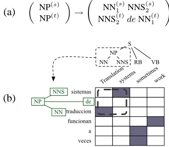
We demonstrate our technique using the syn-chronous grammar formalism of tree-to-tree trans-ducers (Knight and Graehl, 2004). In each weighted rule, an aligned pair of nonterminals generates two ordered lists of children. The non-terminals in each list must align one-to-one to the non-terminals in the other, while the terminals are placed freely on either side. Figure 3(a) shows an example rule.

Following Galley et al. (2004), we learn a gram-mar by projecting English syntax onto a foreign lan-guage via word-level alignments, as in figure 3(b).7

We parsed 1200 English-Spanish sentences using a grammar learned from 40,000 sentence pairs of the English-Spanish Europarl corpus.8 Figure 4(a) shows that A∗ expands substantially fewer states while searching for the optimal parse with our

op-7

The bilingual corpus consists of translation pairs with fixed English parses and word alignments. Rules were scored by their relative frequencies.

8

Rare words were replaced with their parts of speech to limit the memory consumption of the parser.

(a) „

NP(s)

NP(t) «

→ NN

(s)

1 NNS

(s) 2

NNS(2t)deNN (t) 1

!

(b)

Translationsystems sometimeswork

sistemas

traduccion funcionan a veces

de NNS

NN NP

NNS NN

NP

RB VB S

Figure 3: (a) A tree-to-tree transducer rule. (b) An example training sentence pair that yields rule (a).

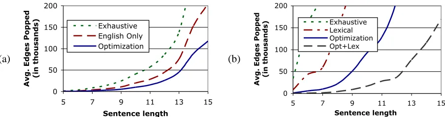
timization heuristic. The exhaustive curve shows edge expansions using the null heuristic. The in-termediate result, labeled English only, used only the English monolingual outside score as a heuris-tic. Similar results using only Spanish demonstrate that both projections contribute to parsing efficiency. All three curves in figure 4 represent running times for finding the optimal parse.

Zhang and Gildea (2006) offer a different heuris-tic for A∗ parsing of ITG grammars that provides a forward estimate of the cost of aligning the unparsed words in both sentences. We cannot directly apply this technique to our grammar because tree-to-tree transducers only align non-terminals. Instead, we can augment our synchronous grammar model to in-clude a lexical alignment component, then employ both heuristics. We learned the following two-stage generative model: a tree-to-tree transducer generates trees whose leaves are parts of speech. Then, the words of each sentence are generated, either jointly from aligned parts of speech or independently given a null alignment. The cost of a complete parse un-der this new model decomposes into the cost of the synchronous tree over parts of speech and the cost of generating the lexical items.

(a)

0 50 100 150 200

5 7 9 11 13 15

Sentence length Avg. Edges Popped (in thousands)

Exhaustive Lexical Optimization Opt+Lex

0 50 100 150 200

5 7 9 11 13 15

Sentence length Avg. Edges Popped (in thousands)

Exhaustive English Only Optimization

(b)

0 50 100 150 200

5 7 9 11 13 15

Sentence length Avg. Edges Popped (in thousands)

Exhaustive Lexical Optimization Opt+Lex

0 50 100 150 200

5 7 9 11 13 15

Sentence length

Avg. Edges Popped

(in thousands)

Exhaustive English Only Optimization

Figure 4: (a) Parsing efficiency results with optimization heuristics show that both component projections constrain the problem. (b) Including a lexical model and corresponding heuristic further increases parsing efficiency.

4 Lexicalized Parsing

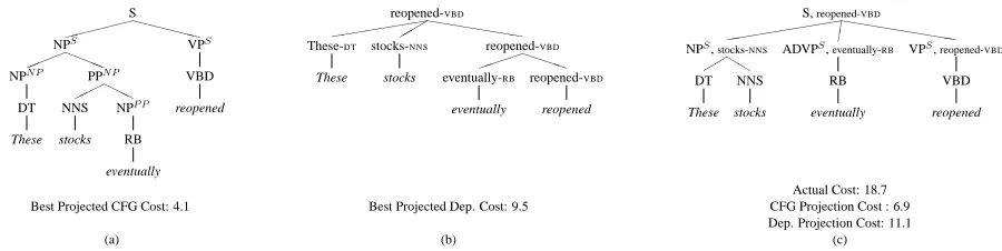
We next apply our technique to lexicalized pars-ing (Charniak, 1997; Collins, 1999). In lexical-ized parsing, the local configurations are lexicallexical-ized rules of the formX[h, t]→ Y[h0, t0]Z[h, t], where h, t, h0, and t0 are the head word, head tag, ar-gument word, and arar-gument tag, respectively. We will user = X → Y Z to refer to the CFG back-bone of a lexicalized rule. As in Klein and Man-ning (2003), we view each lexicalized rule, `, as having a CFG projection, πc(`) = r, and a de-pendency projection, πd(`) = (h, t, h0, t0)(see fig-ure 5).9 Broadly, the CFG projection encodes con-stituency structure, while the dependency projection encodes lexical selection, and both projections are asymptotically more efficient than the original prob-lem. Klein and Manning (2003) present a factored model where the CFG and dependency projections are generated independently (though with compati-ble bracketing):

P(Y[h, t]Z[h0, t0]|X[h, t]) = (6)

P(Y Z|X)P(h0, t0|t, h)

In this work, we explore the following non-factored model, which allows correlations between the CFG and dependency projections:

P(Y[h, t]Z[h0, t0]|X[h, t]) =P(Y Z|X, t, h) (7)

P(t0|t, Z, h0, h)P(h0|t0, t, Z, h0, h)

This model is broadly representative of the suc-cessful lexicalized models of Charniak (1997) and

9

We assume information about the distance and direction of the dependency is encoded in the dependency tuple, but we omit it from the notation for compactness.

Collins (1999), though simpler.10

4.1 Choosing Constraints and Handling Unseen Dependencies

Ideally we would like to be able to solve the op-timization problem in (4) for this task. Unfortu-nately, exhaustively listing all possible configura-tions (lexical rules) yields an impractical number of constraints. We therefore solve a relaxed problem in which we enforce the constraints for only a subset of the possible configurations, A0 _{⊆ A. Once we} start dropping constraints, we can no longer guaran-tee pointwise admissibility, and therefore there is no reason not to also allow penalized violations of the constraints we do list, so we solve (5) instead.

To generate the set of enforced constraints, we first include all configurations observed in the gold training trees. We then sample novel configurations by choosing(X, h, t)from the training distribution and then using the model to generate the rest of the configuration. In our experiments, we ended up with 434,329 observed configurations, and sampled the same number of novel configurations. Our penalty multiplierCwas 10.

Even if we supplement our training set with many sample configurations, we will still see new pro-jected dependency configurations at test time. It is therefore necessary to generalize scores from train-ing configurations to unseen ones. We enrich our procedure by expressing the projected configuration costs as linear functions of features. Specifically, we define feature vectors fc(r) and fd(h, t, h0t0) over the CFG and dependency projections, and

intro-10

S XX

XXXX

NPS

a a

aa ! ! ! !

NPN P

DT

These

PPN P H HH NNS

stocks

NPP P

RB

eventually

VPS

VBD

reopened

reopened-VBD

hhh hhhhh "

" " ( ( ( ( ( ( ( (

These-DT

These

stocks-NNS

stocks

reopened-VBD

P P

PP

eventually-RB

eventually

reopened-VBD

reopened

S,reopened-VBD hhh

hhh_hhh h

( ( ( ( ( ( ( ( ( ( NPS_,stocks-NNS

b b " " DT

These

NNS

stocks

ADVPS_,eventually-RB

RB

eventually

VPS_,reopened-VBD

VBD

reopened

Actual Cost: 18.7

Best Projected CFG Cost: 4.1 Best Projected Dep. Cost: 9.5 CFG Projection Cost : 6.9

Dep. Projection Cost: 11.1

(a) (b) (c)

Figure 5: Lexicalized parsing projections. The figure in (a) is the optimal CFG projection solution and the figure in (b) is the optimal dependency projection solution. The tree in (c) is the optimal solution for the original problem. Note that the sum of the CFG and dependency projections is a lower bound (albeit a fairly tight one) on actual solution cost.

duce corresponding weight vectorswc andwd. The weight vectors are learned by solving the following optimization problem:

minimize γ,wc,wd

kγ+k2+Ckγ−k2 (8)

such that, wc≥0, wd≥0

γ`=c(`)−[wTcfc(r) +wdTfd(h, t, h0, t0)]

for`= (r, h, t, h0, t0)∈ A0

Our CFG feature vector has only indicator features for the specific rule. However, our dependency fea-ture vector consists of an indicator feafea-ture of the tu-ple(h, t, h0, t0)(including direction), an indicator of the part-of-speech type(t, t0) (also including direc-tion), as well as a bias feature.

4.2 Experimental Results

We tested our approximate projection heuristic on two lexicalized parsing models. The first is the fac-tored model of Klein and Manning (2003), given by equation (6), and the second is the non-factored model described in equation (7). Both models use the same parent-annotated head-binarized CFG backbone and a basic dependency projection which models direction, but not distance or valence.11

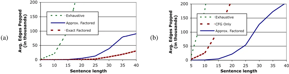
In each case, we compared A∗using our approxi-mate projection heuristics to exhaustive search. We measure efficiency in terms of the number of ex-panded hypotheses (edges popped); see figure 6.12 In both settings, the factored A∗ approach substan-tially outperforms exhaustive search. For the

fac-11

The CFG and dependency projections correspond to the PCFG-PA and DEP-BASIC settings in Klein and Manning (2003).

12

All models are trained on section 2 through 21 of the En-glish Penn treebank, and tested on section 23.

tored model of Klein and Manning (2003), we can also compare our reconstructed bound to the known tight bound which would result from solving the pointwise admissible problem in (4) with all con-straints. As figure 6 shows, the exact factored heuristic does outperform our approximate factored heuristic, primarily because of many looser, backed-off cost estimates for unseen dependency tuples. For the non-factored model, we compared our approxi-mate factored heuristic to one which only bounds the CFG projection as suggested by Klein and Manning (2003). They suggest,

φc(r) = min `∈A:πc(`)=r

c(`)

where we obtain factored CFG costs by minimizing over dependency projections. As figure 6 illustrates, this CFG only heuristic is substantially less efficient than our heuristic which bounds both projections.

encoun-(a)

0 50 100 150 200

5 10 15 20 25 30 35 40

Sentence length Avg. Edges Popped (in thousands)

Exhaustive CFG Only

Approx. Factored

0 50 100 150 200

5 10 15 20 25 30 35 40

Sentence length Avg. Edges Popped (in thousands)

Exhaustive

Approx. Factored

Exact Factored

(b)

0 50 100 150 200

5 10 15 20 25 30 35 40

Sentence length Avg. Edges Popped (in thousands)

Exhaustive CFG Only Approx. Factored

0 50 100 150 200

5 10 15 20 25 30 35 40

Sentence length Avg. Edges Popped (in thousands)

Exhaustive

Approx. Factored

Exact Factored

Figure 6: Edges popped by exhaustive versus factored A∗search. The chart in (a) is using the factored lexicalized model from Klein and Manning (2003). The chart in (b) is using the non-factored lexicalized model described in section 4.

tered during search. For both the factored and non-factored model, less than 2% of the configurations scored by the approximate projection heuristic dur-ing search violated pointwise admissibility.

While this is a paper about inference, we also measured the accuracy in the standard way, on sen-tences of length up to 40, using EVALB. The fac-tored model with the approximate projection heuris-tic achieves an F1of 82.2, matching the performance with the exact factored heuristic, though slower. The non-factored model, using the approximate projec-tion heuristic, achieves an F1of 83.8 on the test set, which is slightly better than the factored model.13

We note that the CFG and dependency projections are as similar as possible across models, so the in-crease in accuracy is likely due in part to the non-factored model’s coupling of CFG and dependency projections.

5 Conclusion

We have presented a technique for creating A∗ es-timates for inference in complex models. Our tech-nique can be used to generate provably admissible estimates when all search transitions can be enumer-ated, and an effective heuristic even for problems where all transitions cannot be efficiently enumer-ated. In the future, we plan to investigate alterna-tive objecalterna-tive functions and error-driven methods for learning heuristic bounds.

Acknowledgments We would like to thank the anonymous reviewers for their comments. This work is supported by a DHS fellowship to the first

13

Since we cannot exhaustively parse with this model, we cannot compare our F1to an exact search method.

author and a Microsoft new faculty fellowship to the third author.

References

E. D. Andersen and K. D. Andersen. 2000. The MOSEK in-terior point optimizer for linear programming. In H. Frenk

et al., editor, High Performance Optimization. Kluwer

Aca-demic Publishers.

Stephen Boyd and Lieven Vandenberghe. 2005. Convex

Opti-mization. Cambridge University Press.

Eugene Charniak. 1997. Statistical parsing with a context-free grammar and word statistics. In National Conference on

Ar-tificial Intelligence.

Michael Collins. 1999. Head-driven statistical models for nat-ural language parsing.

Ariel Felner, Richard Korf, and Sarit Hanan. 2004. Additive pattern database heuristics. JAIR.

Michel Galley, Mark Hopkins, Kevin Knight, and Daniel Marcu. 2004. What’s in a translation rule? In HLT-NAACL. Malik Ghallab and Dennis G. Allard. 1982. A∗ - an efficient

near admissible heuristic search algorithm. In IJCAI. P. Hart, N. Nilsson, and B. Raphael. 1968. A formal basis for

the heuristic determination of minimum cost paths. In IEEE

Transactions on Systems Science and Cybernetics. IEEE.

Dan Klein and Christopher D. Manning. 2003. Factored A* search for models over sequences and trees. In IJCAI. Kevin Knight and Jonathan Graehl. 2004. Training tree

trans-ducers. In HLT-NAACL.

I. Dan Melamed, Giorgio Satta, and Ben Wellington. 2004. Generalized multitext grammars. In ACL.

F. J. Och and H. Ney. 2000. Improved statistical alignment models. In ACL.

Ian H. Witten and Timothy C. Bell. 1991. The zero-frequency problem: Estimating the probabilities of novel events in adaptive text compression. IEEE.

Dekai Wu. 1997. Stochastic inversion transduction grammars and bilingual parsing of parallel corpora. Comput. Linguist. Hao Zhang and Daniel Gildea. 2006. Efficient search for