MÉRA Workshop Proceedings

Editors: Emily Gleeson, Eoin Whelan

Authors: Nicole Beisiegel, Frédéric Dias, Eadaoin Doddy, Lisette Edvinsson, Emily

Gleeson, Edward Graham, Ludvig Isaksson, Frank McDermott, Kristian Pagh Nielsen,

Semjon Schimanke, Conor Sweeney, Per Undén, Jonathan Webb, Eoin Whelan, Liam Woods

This article is provided by the author(s) and Met Éireann in accordance with publisher

policies. Please cite the published version.

Citation:

Gleeson E, Whelan E [editors], Nicole Beisiegel, Frédéric Dias, Eadaoin Doddy,

Lisette Edvinsson, Emily Gleeson, Edward Graham, Ludvig Isaksson, Frank McDermott,

Kristian Pagh Nielsen, Semjon Schimanke, Conor Sweeney, Per Undén, Jonathan Webb, Eoin

Whelan, Liam Woods, ‘MÉRA Workshop Proceedings’, Met Éireann, 2019-12-15.

Although every effort has been made to ensure the accuracy of the material contained in this publication, complete accuracy cannot be guaranteed. Neither Met Éireann nor the author accept any responsibility what-soever for loss or damage occasioned or claimed to have been occasioned, in part or in full, as a consequence of any person acting, or refraining from acting, as a result of a matter contained in this publication. All or part of this publication may be reproduced without further permission, provided the source is acknowledged.

c

Met Éireann 2019

ISSN 1393-905X

Title:MÉRA Workshop Proceedings

Editors:Emily Gleeson, Eoin Whelan

Authors: Nicole Beisiegel, Frédéric Dias, Eadaoin Doddy, Lisette Edvinsson, Emily Gleeson, Edward Gra-ham, Ludvig Isaksson, Frank McDermott, Kristian Pagh Nielsen, Semjon Schimanke, Conor Sweeney, Per Undén, Jonathan Webb, Eoin Whelan, Liam Woods

Contents

Weather observations are routinely used to analyse the past climate. Climate reanalyses may also be used for this purpose. These give a numerical description of the recent climate and are produced by combining models with weather observations. They contain estimates of atmospheric parameters such as air temperature, pressure and wind at different heights above the ground, and surface parameters such as precipitation, soil moisture content and temperatures, and sea-surface temperature. Because they are carried out using a fixed version of a forecast model and a data assimilation system which utilises historical observations, they produce parameters that are physically consistent and often not routinely observed. Thus, climate reanalyses have the potential to extend the knowledge gained from current observation networks.

Over the past few years researchers at Met Éireann have produced a climate reanalysis dataset, called MÉRA - Met Éireann Reanalysis, for the period 1981-2019 for an area covering Ireland, the UK and northern France. This dataset was launched in May 2017 and currently has over 100 users in Ireland, the U.K., Germany, the Netherlands, Canada and the U.S. On May 2nd _{2019 we held the first workshop for users of the data. The}

workshop consisted of 14 very interesting talks spread across three sessions and covering topics such as global and regional reanalysis, atmospheric rivers, renewable energy, waves and extreme storms. Short papers on a selection of these talks are included in this workshop proceedings.

Further scientific information on MÉRA can be found in the following publications:

Gleeson, E., Whelan, E., and Hanley, J.: Met Éireann high resolution reanalysis for Ireland, Adv. Sci. Res.,14, 49-61, https://doi.org/10.5194/asr-14-49-2017, 2017.

https://www.adv-sci-res.net/14/49/2017/asr-14-49-2017.pdf

Whelan, E., E. Gleeson, and J. Hanley: An evaluation of MÉRA, a high resolution mesoscale regional reanal-ysis. J. Appl. Meteor. Climatol.,57, 2179-2196, doi:10.1175/JAMC-D-17-0354.1, 2018.

S. Schimanke et al.

Copernicus Regional Reanalysis for Europe

Semjon Schimanke1_{, Ludvig Isaksson}1_{, Lisette Edvinsson}1_{, and Per Undén}1 1_{Swedish Meteorological and Hydrological Institute}

1 Introduction to the Service

The Copernicus regional reanalysis for Europe (https://climate.copernicus.eu/regional-reanalysis-europe) is produced as part of the Copernicus Climate Change Service (C3S).

The service will be implemented in several steps as illustrated in Figure 1. Firstly, a system developed in the FP7 project UERRA (Undén et al.) will be used to update the existing regional reanalysis (hereafter referred to as RRA) close to real-time. In combination with the RRA produced already by UERRA, the C3S service will offer a consistent RRA from 1961.

Moreover, an improved model version will be developed within C3S. The model will be used to create a pan-European reanalysis at very high resolution (5.5 km) forced by the global ERA5 reanalysis also produced by C3S. Uncertainty estimates of all the output parameters and essential climate variables (ECVs) will be provided in a variety of forms from an Ensemble Data Assimilation. The uncertainty estimtes will have a somewhat lower horizontal resolution than the control deterministic RRA.

Figure 1: Overview of the main objectives.

Finally, the service will provide support and guidance for users. This will be accomplished using video and online tutorials, a selection of best practise examples, and the organisation of user workshops.

2 Available Reanalysis Data

com-Figure 2: Model domain showing the topography and ocean mask (blue).

UERRA-HARMONIE system and at 5.5 km for the MESCAN-SURFEX system. The model domain is shown in Figure 2.

The systems provide four analyses per day - at 0000 UTC, 0600 UTC, 1200 UTC, and 1800 UTC. Between the analyses, forecasts are available at hourly resolution (see Figure 3). At 00 UTC and 12 UTC the forecasts are extended to 30 hours, which makes the long forecasts overlap. Due to some spin-up issues, it is recom-mended for some parameters to use the long forecast lengths rather than the short ones. This is especially the case for precipitation, gustiness and maximum and minimum temperatures. More details can be found in the user guide (Schimanke et al. 2019), which is available via the Copernicus Climate Data Store (CDS, https://cds.climate.copernicus.eu).

More than fifty parameters are available on level types. The data are partly available through Copernicus Climate Data Store (CDS) as well as ECMWF’s MARS system. In the CDS, the data are split into four records. Data can be found on single levels (surface parameters), 24 pressure levels (1000 hPa–10 hPa), eleven height levels (15 m–500 m) and soil levels (14 levels down to 12 m). Data on model levels are available only via MARS. Examples showing how to download the data via CDS, as well as via MARS, can be found in the user guide (Schimanke et al. 2019).

In total, more than 700 TB of data are currently available.

S. Schimanke et al.

3 Quality of the Reanalysis

3.1 Operational Verification

As part of the operational production, the quality of the produced data are checked regularly. For this, a HIRLAM package called monitor is used, which is also used in operational weather prediction. Several standard verification scores are computed and checked, e.g. bias and standard deviation as function of forecast time, scatter plots, and the Hansen Kuipers skill score. In all of these checks, ERA-interim data are included to enable a comparison between the driving global reanalysis and the RRA. For most parameters, e.g. temperature at 2 m, wind speed at 10 m, and precipitation, UERRA data outperform the global reanalysis. There are only a few parameters, such as as relative humidity, where the global reanalysis compares better to observations than the RRA.

The better performance is mainly related to the higher resolution (11 km for UERRA compared to 80 km for ERA-interim), which allows the model to simulate physical processes more realistically and to the assimilation of additional observational data.

3.2 Comparison with Other Products

In addition to the operational-type verification, tests, comparisons and verification in various ways are per-formed. Recently, we started to compare the UERRA data with ERA5, which is now available back to 1979. Figure 4a shows a comparison of the wind speed between both reanalysis products. It shows the mean differ-ence over the winter months (December–February) for the period 2000–2015. The general patterns are quite close to each other. Hence, differences between the datasets are small in general with most of the differences below 0.5 m s−1_{. Areas with greater differences can be found over northern Africa and the Norwegian Sea.}

These are both regions with fewer observational data so a real validation is not possible. More differences can be found in mountainous regions and along the coast lines. These differences are mainly related to different topographies and coastlines, and are related to the lower horizontal resolution of ERA5.

(a) Difference in the 10 m wind speed between UERRA-HARMONIE and ERA5 for the winter

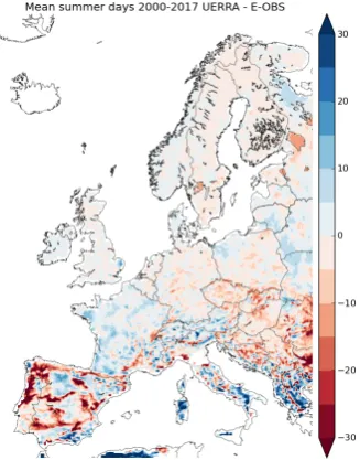
months December to February. (b) Difference in the number of summer days (T2m above25◦C) between UERRA-HARMONIE and E-OBS data.

Table 1: Verification of wind speed by comparison with hourly station data from 24 Swedish stations along the Swedish coastline.

UERRA ERA5 Mean bias -0.02 0.01 Correlation 0.85 0.85 RMSE 1.83 1.97

Along the coastline, an alternating pattern is often seen with stronger winds over water and weaker winds inland (Figure 4a). These patterns are related to differences in the land-sea-masks used in ERA5 and UERRA. We compared the performance of the wind speed for stations along the Swedish coastline. For 24 Swedish stations we computed the bias, the correlation and the root mean square error (RMSE) using hourly data for the period 2000–2015. Both datasets perform almost equally as good. The mean bias over all 24 stations is close to zero and the correlation, based on hourly values, is 0.85 for both datasets. In terms of RMSE, UERRA performs slightly better than ERA5 (Table 1).

Figure 4b shows a comparison of the mean annual number of summer days in UERRA compared with the E-OBS gridded dataset version 17.0 (Cornes et al., 2018). Summer days are days with a maximum 2 m tem-perature above25◦C. Blue colors indicate that UERRA simulates more summer days than E-OBS whereas

red colors indicate that we count more summer days in E-OBS. Once again, areas with higher topography are highlighted in the comparison. Here, regions with overestimation and underestimation are often close to each other implying that such differences depend strongly on the applied topography of the datasets. Since E-OBS can be used as a benchmark dataset when it comes to daily maximum temperatures, we consider it as a success for the RRA that both datasets resemble each other to a large degree.

Additional comparisons - though not to ERA5 - can be found in the UERRA reports (Undén et al.) as well as in Borsche et al. (2015).

3.3 Homogeneity over Time

Investigations of the homogeneity over time were made by Krämer (2018). It was shown that the switch from using ERA40 to ERA-interim for lateral boundary conditions in 1979 has an impact on the quality of the RRA. The investigated forecast skill of the 30 hour minus the 6 hour forecasts improves significantly with this change. Moreover, a general quality increase was noticed over time especially for the upper atmosphere. This trend is a consequence of the growing number of observations, which became available to the assimilation system throughout time. A major source of additional observations comes from automatic aircraft measurements. More information about the homogeneity over time is available in Krämer (2018).

4 Conclusions and Outlook

The operational C3S service for the production of a regional reanalysis for Europe was introduced. An overview of the available data was given as well as the quality of the data using examples. More detailed investigations can be found in Unden et al. In general, we concluded that the RRA outperforms global reanalysis products in most aspects.

S. Schimanke et al.

dataset covering the period from the early 1980 should be available at the end of summer 2021.

5 Acknowledgments

The operational updates of the UERRA reanalysis data are produced as part of the Copernicus Climate Change Service (C3S) under contract C3S_322_Lot1.

6 References

Borsche, M, A. K. Kaiser-Weiss, P. Undén, and F. Kaspar: Methodologies to characterize uncertainties in regional reanalyses.Adv. Sci. Res.,12, 207–218, https://doi.org/10.5194/asr-12-207-2015, 2015.

Copernicus Climate Change Service (C3S): ERA5: Fifth generation of ECMWF atmospheric reanalyses of the

global climate . Copernicus Climate Change Service Climate Data Store (CDS), July 2019. https://cds.climate.copernicus.eu/cdsapp#!/home, 2017.

Cornes, R., G. van der Schrier, E.J.M. van den Besselaar, and P.D. Jones: An Ensemble Version of the E-OBS Temperature and Precipitation Datasets,J. Geophys. Res. Atmos.,123. doi:10.1029/2017JD028200, 2018. Dee, D. P. et al.: The ERA-Interim reanalysis: configuration and performance of the data assimilation system, https://doi.org/10.1002/qj.828, 2011.

von Krämer, Adam: Temporal consistency of the UERRA regional reanalysis: Investigating the forecast skill, Degree Project at the Department of Earth Sciences, ISSN 1650-6553 Nr. 422,www.diva-portal.org, 2018. Schimanke, S., L. Isaksson, L. Edvinsson, P. Undén, M. Ridal, P. Le Moigne, E. Bazile, A. Verrelle and M. Glinton: UERRA data user guide - version 3.1, pages 49, available e.g. at

Copernicus Climate Change Service (C3S) Arctic regional reanalysis

Kristian Pagh Nielsen1_{and The C3S Arctic regional reanalysis project team}2 1_{Danish Meteorological Institute}

2_{A large group of scientists at: The Norwegian Meteorological Institute (MET), The Danish} Meteorological Institute (DMI), The Swedish Meteorological and Hydrological Institute (SMHI), The Icelandic Meteorological Office (IMO), Météo France (MF) and The Finnish Meteorological

Institute (FMI). See also the acknowledgements.

1 Introduction

With the ERA5 reanalysis (Hershbach & Dee, 2016) having recently become available one may ask, why is a regional reanalysis needed? For the Arctic regions covered by the Norwegian, Icelandic and Danish realms, the answer is that high model resolution is of the essence. Ice sheets, ice caps and mountain glaciers carve out vertical-walled u-shaped valleys and fjords. In order to resolve the weather and climate in these steep land-scapes, high resolution is needed. ERA5 has a 31 km horizontal grid-spacing, while the C3S Arctic regional reanalysis data has a 2.5 km horizontal grid-spacing. Our modelling domains contain the 4 largest bodies of land ice in the Arctic: The Greenland Ice Sheet, the Serverny Island Ice Cap, Vatnajökull and Austfonna. Tests with the HARMONIE-AROME weather model has shown that running this using 2.5 km grid-spacing gives improved wind forecasts for Greenlandic weather stations compared with the previously used opera-tional Greenland weather model HIRLAM which was run on a grid of ˜5 km grid-spacing (Yang et al., 2018). HARMONIE-AROME reanalysis results for other regions have also shown very good results as compared with the previously available coarse resolution reanalysis products. One example is the Met Éireann reanalysis for Ireland and the United Kingdom (Gleeson et al., 2017; Whelan et al., 2018).

The warming in the Arctic, due to increased amounts of atmospheric greenhouse gasses, is occuring at a rate roughly twice as fast as the warming at lower latitudes. The strong decrease seen in the sea ice of the Arctic Ocean both changes the weather and climate patterns in the Arctic region and increases the economic activity in the region - both regarding shipping transport and resource mining. Finally, the Arctic glaciers have retreated strongly since the turn of the millennium (e.g. Box & Decker, 2011). All in all a high resolution regional reanalysis of the Arctic, with state-of-the-art limited area weather models, is in demand.

K. P. Nielsen et al.

2 System Configuration

The HARMONIE-AROME Arctic reanalysis covers the two domains shown in Figure 1. The western "IGB" domain covers Iceland and Greenland and has a size of 1080×1280 grid columns. The eastern "AROME-Arctic" domain covers Northern Scandinavia, Svalbard, Novaya Zemlya, Franz Josef Land and the surrounding seas. It has a size of 800×1000 grid columns. Each grid column in both domains has the dimensions 2.5 km

×2.5 km and has 65 vertical model levels with the lowest model level being approximately 12 m above the surface and the highest model level being at 10 hPa (Undén, 2010). The model is run in 3-hourly cycles 8 times each day with 30 hour forecasts being made at 0000 and 1200 UTC. The modelling domains are nested within ERA5, from which hourly lateral boundary conditions are used. The model output is provided on an hourly basis. Initially the reanalysis will be performed for the 24 year period from April 1997 to April 2021.

Figure 1: The C3S Arctic regional reanalysis domains. The western domain is a common Danish-Icelandic (IGB) modelling domain, while the eastern domain is a Norwegian (AROME-Arctic) modelling domain cover-ing Svalbard, the Barents Sea and Northern Scandinavia.

A modified version of the HARMONIE-AROME model cycle 40h1.1.1 is used, where a special emphasis has been made regarding frozen surfaces such as snow, sea ice and glaciers. For sea ice modelling the SICE sea ice scheme is used (Batrak et al., 2018). The model has also been improved by adding a large amount of new observational data, which were not included in the ERA-5 reanalysis, and which have not yet been included in the Global Telecommunication System (GTS) of the World Meteorological Organization (WMO). In particular these data are local Arctic observational data from Denmark, Norway, Iceland, Sweden and Finland. Data from other scientific institutions have also been included. These input data are summarised in section 3.

The data assimilation code of the modelling system has been adapted to use these data. The upper air (3DVar) data assimilation system has been updated so that atmospheric variables measured from satellites, aircraft, surface pressure sensors and radiosondes can be used over the Arctic. Randriamampianina et al. (2019) describe the impact of upper air data assimilation in HARMONIE-AROME for Arctic regions.

3 Input Data

In Figure 2 the amount of additional synoptic weather stations relative to the GTS stations is illustrated for Iceland and Greenland. In particular more observations over the Greenland ice sheet from the GC-Net (2C) (Steffen et al., 1996) and PROMICE stations (2D) (van As et al., 2011) have been added.

Figure 2: GTS and additional synoptic weather station data that are included for Greenland and Iceland. A: GTS stations (blue and blue-red points) and additional Icelandic stations (red points). B: Greenlandic Asiaq stations.C: GC-Net stations.D: PROMICE stations.

As mentioned in section 2 we also use extensive satellite remote sensing data of atmospheric temperature, hu-midity and winds. These variables are derived from measurements of radiances, radio occultation, atmospheric motion vectors, and scatterometer data (Schyberg et al., 2013; Randriamampianina et al., 2019).

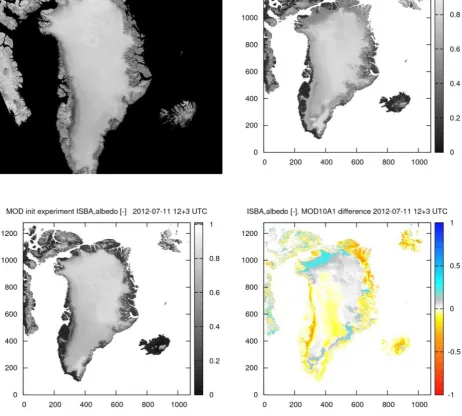
We have also corrected major ice sheet extent and coastline errors for both modelling domains. A common error is that Eastern and Northeastern Greenland is assumed to be entirely covered by the ice sheet (pers. comm. Mottram, 2010). As shown in Figure 3a this error can also be found in the ERA5 renalysis dataset (pers. comm. Palmason, 2018). In Figure 3 plots of the surface albedo on the 31st _{of July 2012 are used to}

show the extent of the glaciated areas in Greenland and the surrounding areas. On the left albedo data from ERA5 are shown, while the 500 m resolution MOD10A1 C6 dataset (Stroeve et al., 2006), that is based on MODIS Terra satellite observations, is shown on the right hand side. The errors in the ERA5 glacier extent for Eastern and Northeastern Greenland are large. Some smaller errors can also be seen in the MOD10A1 C6 product, where for instance the Storstømmen glacier in Eastern Greeland is missing.

K. P. Nielsen et al.

(a) ERA5 albedo 2012-07-31 12 UTC. (b) MODIS (MOD10A1 C6) albedo 2012-07-31.

Figure 3: Comparison of glacier masks illustrated with albedo data for Greenland and surroundings.

Figure 4: Example of coastline errors for the northernmost part of Greenland. Here the official coastline from the Danish Map Supply is compared with the previously used GTOPO30 dataset.

and sand and clay soil fractions from the SoilGrids database (Hengl et al., 2017) have been implemented for all Arctic areas except Iceland, for which local sand and clay data are used.

The albedo of the glaciers controls the energy absorbed by these at the surface level. It also affects the whole atmospheric state – including the energy fluxes and winds. It is very complicated to model the albedo of glaciers correctly, since a large number of factors affect this including internal glacial impurities, aerosol deposits, snow-grain size changes, surface hoar and algae. Figure 5 illustrates how different the albedo can be for a specific day from one year to another. The glacier albedo also can vary a lot from day to day. To accommodate this variability we use a daily gridded and gap-filled version of the MOD10A1 C6 product (Box & van As, 2017). The gap-filling includes keeping the albedo constant for days on which clouds obscure the surface, and spacial and temporal smoothing to reduce noise in the data.

Figure 5: Greenland albedos from MOD10A1 collection 6 for the same day in two different years.A: July 1st

2000.B: July 1st_2012.

4 Results and Discussion

The project started in September 2017. Since September 2018 beta testing has been performed with the aim of deciding which system improvements and input data that should be included in the final system configuration for the reanalysis. The results shown here are from this beta testing.

K. P. Nielsen et al.

Figure 6 shows how assimilating CryoClim snow cover improves the temperature reanalysis for Svalbard. Similar tests have been performed for all seasons for both model domains for each of the updates added to the reference system configuration.

Figure 7: Results from an experiment using daily gap-filled MOD10A1 C6 albedos. MOD10A1 C6 input data (upper left), alpha-version reference HARMONIE-AROME albedo (upper right), albedo when assimilating the MOD10A1 C6 albedos in HARMONIE-AROME (lower-left) and absolute albedo difference relative to the reference experiment (lower-right).

satellite product often will not detect such an albedo-increase on the day it happens due to obscuring clouds, this is a desirable feature.

Figure 8: Comparison of analysed and measured surface temperatures at the PROMICE station "QAS_L" for a reference experiment labelled "alpha2" and an experiment in which the MOD10A1 C6 albedos were assimilated labelled "beta2". The QAS_L station is situated near the South Greenland village of Qassimiut (61.02◦_{N, 46.84}◦_W).

Figure 9: Frequency distribution of the model to measurement differences for the albedo (left) and the surface temperatures (right) for the reference "alpha2" model run. Data from all PROMICE stations from the month of July 2012 are included.

In Figures 8–10 the impact of assimilating the MOD10A1 C6 albedos for the Greenland ice sheet is shown where the error distributions have lower mean values and lower standard deviations. Figure 9 shows the statis-tics for the reference "alpha2" experiment in which no albedos have been assimilated, while Figure 10 shows the statistics for the "beta2" experiment, which includes the albedo assimilation for the glaciers. The statistics are shown as frequency distributions of the absolute difference of the modelled and observed data, albedos (left) and surface temperatures (right). In theseµdenotes the mean values of the frequency distributions, andσ

denotes the standard deviations of these.

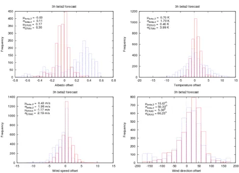
Finally, the C3S Arctic reanalysis should of course be better than the ERA5 reanalysis. Statistical comparisons of albedo, surface temperature, wind speed and wind direction are shown in Figure 11. Again the statistics for each of these variables is shown in the form of frequency distributions. July 2012 data from all operational PROMICE stations on the Greenland Ice Sheet (Figure 2D) are included in these distributions.

K. P. Nielsen et al.

Figure 10: As for 9 but for the MOD10A1 C6 "beta2" experiment.

Figure 11: Frequency distributions of both the HARMONIE-AROME "beta2" experiment (red columns) and ERA5 data (blue columns) differences to measurement data – upper-left (A): albedo, upper-right (B): sur-face temperatures, lower-left (C): wind speed, and lower-right (D): wind direction. Data from all operational PROMICE stations from the month of July 2012 are included.

For the wind speeds (Figure 11C), the mean value of the deviation is reduced from -1.2 m s−1 _{(ERA5) to}

0.4 m s−1_{(HARMONIE-AROME), and the standard deviation is reduced from 2.2 m s}−1_{(ERA5) to 2.0 m s}−1

(HARMONIE). Note here that the PROMICE stations do not measure the wind speed at the regular 10 m height, instead at a 1–3 m height depending on the snow depth. Therefore, we correct the modelled wind speeds at 10 m to the boom heights with the method described by Mottram et al., (2017). For the wind directions (Figure 11D), the standard deviation is reduced from 66◦ _{to 50}◦_{, but the mean deviation increases from 5}◦ _{to 16}◦_{. Here the}

issues is again very likely to be the comparison of grid-box average wind directions with a local measurement. Since katabatic winds are prevalent on the Greenland Ice Sheet, the local slope, to a large extent, determines the wind direction, and this slope will often differ from the grid-box average slope. Additionally, a measurement alignment uncertainty exists that arises from the practical challenge of aligning a station to geographic north in a part of the world that is close to the magnetic north pole (pers. comm. Fausto, 2019).

5 Conclusions and Future Work

We have successfully designed a reanalysis system for the Arctic which includes many new local ground-based and satellite data sources. After choosing the system configuration and input data that is used in the reanalysis, the production of this was started in Spring 2019. The production is done in several time slices in parallel, each with one year of spin-up time as suggested by Gleeson et al. (2017). The data will be available via the Copernicus Data Service (CDS) by the Summer of 2021. Additionally, one full year of reanalysis data will be made for a domain that covers the entire Arctic region.

6 Acknowledgments

K. P. Nielsen et al.

7 References

Batrak, Y., E. Kourzeneva, and M. Homleid: Implementation of a simple thermodynamic sea ice scheme, SICE version 1.0-38h1, within the ALADIN-HIRLAM numerical weather prediction system version 38h1,

Geosci. Model Dev.,11, 3347–3368, doi:10.5194/gmd-11-3347-2018, 2018.

Bengtsson, L., Andrae, U., Aspelien, T., Batrak, Y., Calvo, J., de Rooy, W., Gleeson, E., Sass, B. H., Homleid, M., Hortal, M., Ivarsson, K.-I., Lenderink, G., Niemelä, S., Nielsen, K. P., Onvlee, J., Rontu, L., Samuelsson, P., Santos Muñoz, D., Subias, A., Tijm, S., Toll, V., Yang, X., and Køltzow, M. Ø.: The HARMONIE-AROME Model Configuration in the ALADIN-HIRLAM NWP System,Mon. Weather Rev.,145, 1919–1935,

doi:10.1175/MWR-D-16-0417.1, 2017.

Box, J. E.X and D. T. Decker: Greenland marine-terminating glacier area changes: 2000-2010, Annals of Glaciology,52(59), 91–98, doi:10.3189/172756411799096312, 2011.

Box, J.E., D. van As, K. Steffen: Greenland, Canadian and Icelandic land ice albedo grids (2000–2016). Geo-logical Survey of Denmark and Greenland Bulletin,38, 53–56, 2017.

Gleeson, E., E. Whelan, and J. Hanley: Met Éireann high resolution reanalysis for Ireland,Adv. Sci. Res.,14, 49–61, doi:10.5194/asr-14-49-2017, 2017.

Hengl, T., Mendes de Jesus, J., Heuvelink, G. B.M., Ruiperez Gonzalez, M., Kilibarda, M. et al.: Soil-Grids250m: global gridded soil information based on Machine Learning. PLoS ONE 12 (2), e0169748, doi:10.1371/journal.pone.0169748, 2017.

Hersbach, H., and E. Dee: ERA5 reanalysis is in production,ECMWF Newsletter,147, 7, 2016.

Mottram, R., K. P. Nielsen, E. Gleeson, and X. Yang: Modelling Glaciers in the HARMONIE-AROME NWP model.Adv. Sci. Res.,14, 323–334, doi:10.5194/asr-14-323-2017, 2017.

Nielsen-Englyst, P., J. L. Høyer, L. Toudal Pedersen, C. L. Gentemann, E. Alerskans, T. Block, and C. Donlon: Optimal Estimation of Sea Surface Temperature from AMSR-E.Remote Sens.,10(2), 229,

doi:10.3390/rs10020229, 2018.

Norwegian Polar Institute: Kartdata Svalbard 1:100 000 (S100 Kartdata) Map Data. Norwegian Polar Institute. doi:10.21334/npolar.2014.645336c7, 2014.

Randriamampianina, R., H. Schyberg, and M. Mile: Observing System Experiments with an Arctic Mesoscale Numerical Weather Prediction Model,Remote Sens.,11, 981, doi:10.3390/rs11080981, 2019.

RGI Consortium: Randolph Glacier Inventory – A Dataset of Global Glacier Outlines: Version 5.0: Technical Report, Global Land Ice Measurements from Space, Colorado, USA. Digital Media. doi:10.7265/N5-RGI-50, 2015.

Scarlat, R.C., G. Heygster, L. T. Pedersen: Experiences with an Optimal estimation algorithm for surface and atmospheric parameter retrieval from passive microwave data in the arctic. IEEE J. Sel. Top. Appl. Earth Obs. Remote Sens.,10, 3934–3947, doi:10.1109/JSTARS.2017.2739858, 2017.

Schyberg, H., T. Nipen, and R. Randriamampianina: Arctic forecast quality and assessment of state and im-pacts of the components of the Arctic observing system. Deliverable Report,D1-81, Arctic Climate Change, Economy and Society (ACCESS), EU Seventh Framework Programme (FP7), 2013.

Seity, Y., P. Brousseau, S. Malardel, G. Hello, P. Benard, F. Bouttier, C. Lac, and V. Masson: The AROME-France Convective-Scale Operational Model.Mon. Weather Rev.,139, 976–991,

doi:10.1175/2010MWR3425.1, 2011.

Steffen, K., J. E. Box, and W. Abdalati: Greenland Climate Network: GC-Net, in: Colbeck, S. C. (ed.): Glaciers, Ice Sheets and Volcanoes: A Tribute to Mark F. Meier. Cold Regions Research & Engineering Laboratory, U.S. Army Cops of Engineers, Hanover, NH 03755, USA, 98–103, 1996.

Stroeve, J. C., J. E. Box, and T. Haran: Evaluation of the MODIS (MOD10A1) daily snow albedo product over the Greenland ice sheet.Rem. Sens. Environ.,105(2), 155–171, doi:10.1016/j.rse.2006.06.009, 2006.

Undén, P.: Revised method of determination of the hybrid coordinate in HIRLAM.HIRLAM Newsletter,56, 30–36, 2010.

van As, D., Fausto, R.S., Ahlström, A.P., Andersen, S.B., Andersen, M.L., Citterio, M., Edelvang, K., Gravesen, P., Machguth, H., Nick, F.M., Nielsen, S., and Weidick, A: Programme for Monitoring of the Greenland Ice Sheet (PROMICE): first temperature and ablation record. Geological Survey of Denmark and Greenland Bul-letin,23, 73–76, 2011.

Whelan, E., E. Gleeson, and J. Hanley: An evaluation of MÉRA, a high resolution mesoscale regional reanal-ysis.J. Appl. Meteor. Climatol.,57, 2179–2196, doi:10.1175/JAMC-D-17-0354.1, 2018.

E. Graham, J. Webb

Extreme Low Thicknesses during the ‘Beast from the East’ of 2018

1_{University of the Highlands and Islands, Scotland}

2_{The Tornado and Storm Research Organisation (TORRO), Oxford}

1 Introduction

During the winter season, the thickness of the 1000-500 hPa atmospheric layer, together with 850 and 500 hPa air temperatures, is traditionally used by operational meteorologists and synoptic climatologists to describe the intensity and severity of surface to mid-troposphere cold cools across the polar and mid-latitudes (e.g. Pike, 1990; Pike and Webb, 2011). The various reanalyses can therefore be used to provide a comprehensive and long-term climatology of such features for different geographical regions, as well as give an indication of any changes in their temporal or spatial frequency.

Based on an earlier study of 1000-500 hPa thicknesses from the NCEP/NCAR (Kalnayet al. 1996), NCEP DOE2 (Kanamitsu et al. 2002) and NOAA-CIRES 20CR (Compo et al. 2011) reanalyses, together with 850/500 hPa air temperature fields, Graham and Webb (2019) have already shown that the infamous ‘Beast from the East’ of 2018 was one of the most severe easterly cold pools to have crossed the UK and Ireland over the past 70-102 years.

This brief additional study compares radiosonde measurements, the NCEP/NCAR and NCEP DOE2 Reanaly-ses, and the much higher spatial resolution MÉRA reanalysis (Gleesonet al. 2017; Whelanet al., 2018) during the easterly cold pool phase of the ‘Beast from the East’ of 2018.

2 Methodology

Figure 2: NCEP-NCAR Reanalysis II 1000-500 hPa thickness for 00 UTC, 28 Feb 2018

Thicknesses were similarly determined for the complete geographical domain as shown in Figure 2, and for the full period of each reanalysis product. Thickness occurrences of less than 5080 metres (508 decametres, dam) were specifically noted. The equivalent 850 hPa and 500 hPa air temperature values were also extracted for the same temporal and spatial co-ordinates.

3 Results

Full quantitative agreement was obtained between MÉRA and measurements by radiosonde over Albemarle, Northumberland (England) on 28 February 2018 (Figure 3). Here, a new UK lowest 500 hPa air temperature record of -46 degrees was measured by the radiosonde at 1200 UTC. Although probably not independent, this extreme radiosonde value is confirmed by the MÉRA value of 228 K at the same time.

E. Graham, J. Webb

Figure 3: MÉRA 500 hPa air temperature, for 12 UTC on 28 Feb 2018. Dark blue colours indicate values below 228 K (-45 degrees), confirming the record low radiosonde value of -46 degrees measured at Albemarle, Northumberland, England at the same time.

4 Conclusions

This brief piece of work, supplementing the earlier and original work of Graham and Webb (2019), insofar as 500 hPa air temperature is considered, confirms that MÉRA fully captures the extreme intensity and local mesoscale features of the ’Beast from the East’ event of 2018.

5 References

Compo, G.P., Whitaker, J.S., Sardeshmukh, P.D., Matsui, N., Allan, R.J., Yin, X., Gleason, B.E., Vose, R.S., Rutledge, G., Bessemoulin, P. and S. BrÃ˝unnimann: The twentieth century reanalysis project. Quarterly Journal of the Royal Meteorological Society,137(654), 1–28, 2011.

Gleeson, E., Whelan, E., and Hanley, J.: Met Éireann high resolution reanalysis for Ireland,Adv. Sci. Res.,14, 49–61, https://doi.org/10.5194/asr-14-49-2017, 2017.

Graham, E. and J.D. Webb: The very deep cold pool of 27 Februaryâ ˘A¸S1 March 2018â ˘A¸Shistorical precedents and perspective.Weather,74(3), 85–91, 2019.

DOE AMIP-II reanalysis (R-2).Bulletin of the American Meteorological Society,83(11), 1631–1644, 2002. Pike, W.S.: Persistent coastal convergence in a heavy snowfall event on the south-east coast of England. Mete-orological Magazine,119, 21, 1990.

Pike W.S, and J.D.C. Webb: An historical and climatological note on snowfalls associated with cold pools in southern Britain.Weather,66, 16â ˘A¸S19, 2011.

L. Woods

The Identification of Persistent Atmospheric Rivers & Associated

Precipitation Events in Ireland

Liam Woods1

1_{University College of Dublin}

1 Introduction

Atmospheric rivers (ARs) are narrow, filament-like structures of intense water vapour flux in the lower tropo-sphere. At any given time, more than 90% of the total poleward water vapour transport through the mid-latitudes is contained within 4 or 5 of these atmospheric rivers, which take up less than 10% of the circumference of the Earth at any given latitude. They are characterised as being thousands of kilometers long, and no more than 500 km wide, and have both high concentrations of integrated water vapor (IWV) and strong low level winds. These narrow corridors transport water vapor from the tropics to the mid-latitudes, and can cause precipitation once they encounter orography.

In the past 20 years, there has been an upsurge in research on the topic of atmospheric rivers, and their link to extreme precipitation events in particular countries, including the west coast of North America, the U.K., and the Iberian Peninsula. In the case of California, it has been shown that ARs were linked to flooding of the Russian River (Ralph et al., 2006), and later it was shown that ARs directly contributed to up to 50% of the total landfall precipitation in California on average (Dettinger et al., 2011). For European countries, ARs typically have a smaller impact. In the U.K. it has been shown that ARs were present for all of the top 10 winter flooding events in 4 separate river basins (Lavers et al., 2011). However, a follow-up study has shown that ARs do not explain extreme rainfall in the summer (Champion et al., 2015), so there is seasonal variation to consider. In this project, the link between ARs and extreme precipitation events in Ireland will be investigated using both the ERA5 dataset to identify ARs, as well as the MÉRA dataset (Gleesonet al. 2017; Whelanet al., 2018) for the precipitation field.

2 Data and Methods

Due to the scale of ARs, it was necessary to observe a larger domain than MÉRA in order to identify them. The ERA5 data used for this project was obtained from the Copernicus Climate Change Service data store, at 8 hour time intervals for a 30 year period between 1981-2010.

2.1 Atmospheric River Detection Algorithm

The first algorithm for identifying ARs was proposed by Zhu & Newell (1998), and this paved the way for more modern techniques which are used widely today (Lavers et al., 2012; Ramos et al., 2015). This method is largely the same across all papers and is the one that will be used for this project. Here are the steps that were taken:

The ERA5 reanalysis data (30 km horizontal grid spacing) was used to obtain specific humidityq, as well as the zonal and meridional wind speeds,uandv, at the 1000, 925, 850, 700, 600, 500, 400, and 300 hPa levels. These fields are used to calculate the integrated vapour transport (IVT) field using equation 1.

IV T =

v u u t 1

g

Z 300hP a

1000hP a qu dp

!2

+ 1

g

Z 300hP a

1000hP a qv dp

!2

(1)

where g denotes acceleration due to gravity, anddp is the pressure difference between two adjacent levels. Once the IVT field has been calculated, the data are split into 12 bins, one per month. This was done to reflect the seasonal variation in IVT values. The 85th percentile of each month was calculated for all grid points. This is the threshold that must be exceeded before a grid point is considered to be part of an AR. Figure 1 shows the seasonal variation in a grid point off the west coast of Ireland, with the blue point representing the 85th percentile of each month. Figure 2 shows this also, over the entire domain by looking at the 85th percentile in June and December.

A line of grid points is needed to start the detection algorithm. This is the line an atmospheric river must cross in order to be considered. The grid points are chosen to be off the west coast of Ireland, along the 10.5◦_{W meridian, between 51}◦_-55.5◦_{N. For each time-step, the maximum value along this line is found. If}

the maximum value exceeds the 85th percentile threshold for that grid point, then the process is repeated, but this time with using the adjacent grid points above, below and to the left. The points diagonally left are also considered, giving a total of 5 new grid points. The algorithm stops when the maximum value of the adjacent points is no longer above the 85th percentile threshold. The distance between the first and last points is calculated using the latitude and longitude of each, and this must exceed 2000 km for the time-step to be considered an AR time-step.

The list of atmospheric rivers is further limited to those that are considered persistent. A persistent AR is one that lasts at least 2 time-steps (16 hours). Finally, for an AR to be considered independent, 24 hours needs to have passed since the last AR.

2.2 Classification of Extreme Precipitation Events L. Woods

(a) (b)

Figure 2: Spatial plot of 85th percentile threshold

2.2 Classification of Extreme Precipitation Events

In order to investigate the association between ARs and extreme precipitation events, we need to first classify what an extreme precipitation event is. A recent study (Ramos et al. 2018) proposed a classification method that allows us to rank each day in our data set in order of severity, based off of the intensity of the precipitation and the area affected. Using this method, that we can examine 100 of the most severe precipitation events, with the extreme precipitation events being at the top of the list.

This method begins by finding the 95th percentile threshold for Total Precipitation, for each grid point, for each month, in the same way as before. Using these threshold values, the following three quantities were calculated per day:

• A = Area. This is a fraction of the total amount of grid points that exceeded the threshold.

• M = Mean Anomaly. For each grid point that exceeded the threshold, the threshold was taken away from

the value to find the anomaly. This is the average of all those anomalies.

• R = A*M. This effectively averages the Mean Anomaly over the whole Area in question, giving us a

single value to rank the severity of the precipitation that day.

Only grid points that were over the island of Ireland were considered. The precipitation events were ranked with the highest value of R representing the most extreme precipitation event in the 30 year period. The top 100 events were found for the following subsets of the data: winter (Dec,Jan,Feb), extended winter (Oct-Mar), extended summer (Apr-Sep), and summer (Jun,Jul,Aug).

3 Results

By using the AR detection algorithm, there were a total of 642 persistent atmospheric rivers found over the 30 year period. Figure 3 shows the detection algorithm identifying an atmospheric river, with the green line representing the maximum values that exceeded the 85th percentile.

As stated previously, the top 100 precipitation events were chosen for 4 different subsets of the data. Here is a table of the values obtained for the top 5 precipitation events in the winter months:

Table 1: The Top 5 Precipitation Events for the winter months

Date A= Area M= Mean Anomaly (mm) R= A*M (mm)

7th January 2005* 0.829 16.06 13.32

27th January 1985 0.8722 12.59 10.98

12th January 1988* 0.8871 11.66 10.35

6th February 1990* 0.6605 14.52 9.59

16th December 1989 0.8087 10.29 8.32

Here, dates in bold and marked with an asterisk have an associated atmospheric river. In contrast, only 1 of the top 5 precipitation events during the summer months have an associated AR. This suggests that atmospheric rivers are linked to extreme precipitation events in the winter months, but not the summer. If we look instead at the top 100 events for each subset, we see a similar pattern.

Table 2: Relative Frequencies For All Four Subsets

winter ONDJFM AMJJAS summer

P(AR) 563 / 2707 = 0.208 1086 / 5467 = 0.199 934 / 5490 = 0.170 513 / 2760 = 0.186 P(Top 100) 100 / 2707 = 0.037 100 / 5467 = 0.018 100 / 5490 = 0.018 100 / 2760 = 0.036 P(AR | Top 100) 40 / 100 = 0.400 38 / 100 = 0.380 20 / 100 = 0.200 17 / 100 = 0.170 P(Top 100 | AR) 40 / 563 = 0.071 38 / 1086 = 0.035 20 / 934 = 0.021 17 / 513 = 0.033

By comparing row 2 and 4 from this table, we can see that the relative frequency of severe precipitation events doubles given that a day has an associated atmospheric river, but only in the winter and extended winter subsets. For the summer subsets, there is effectively no change in the relative frequency whether there is an atmospheric river or not.

(a) (b)

L. Woods

The final result from this project is from a plot of the average total precipitation for days with severe precip-itation and an associated atmospheric river, and the same plot, but with severe precipprecip-itation days without an associated AR, given in figure 4. For days with an associated AR, there seems to be a higher concentration of severe precipitation in mountainous areas on the west coast. This could be used to identify areas that are likely effected by ARs more heavily, and if these areas were weighted more heavily in the ranking scheme, we might see higher proportions of ARs in the top ranked precipitation events. There also seems to be two strong tracks that ARs follow, one coming in from the West, and the other from the southwest, which warrants further investigation.

4 Conclusions and Future Work

In this project, we have identified a total of 642 persistent atmospheric rivers that have hit Ireland between 1981 and 2010. These atmospheric rivers are linked to 40% of the top 100 precipitation events in the winter months, but less than 20% of the top 100 precipitation events in the summer. By considering conditional probabilities, the data suggests that given there is an AR present, the probability of a top 100 precipitation event occurring in the winter months doubles. However, in the summer, the presence of an AR has no such effect on the probability, suggesting that there is no link between atmospheric rivers and summer time extreme precipitation events. Future work includes focusing on the west coast of Ireland, particularly in mountainous areas, as they seem to be more affected by atmospheric rivers than the east coast.

The AR tracking algorithm used in this project primarily searched in a westerly direction, but as seen in Figure 4, there seems to be strong AR tracks coming from the south, so it is worth also trying the algorithm in that direction and seeing if we pick up more ARs that we missed here.

5 References

Champion, A., Allan, R., and Lavers, D.: Atmospheric rivers do not explain UK summer extreme rainfall,J. Geophys. Res. Atmos.,120, 6731-6741, https://doi.org/10.1002/2014JD022863, 2015.

Dettinger, M.,Ralph, F., Das, T., Neiman, P., and Cayan, D.: Atmospheric rivers, floods and the water resources of California,Water,3, 445-478, https://doi.org/10.3390/w3020445, 2011.

Gleeson, E., Whelan, E., and Hanley, J.: Met Éireann high resolution reanalysis for Ireland,Adv. Sci. Res.,14, 49–61, https://doi.org/10.5194/asr-14-49-2017, 2017.

Lavers, D., Allan, R., Wood, E., Villarini, G., Brayshaw, D., and Wade, A.: Winter floods in Britain are connected to atmospheric rivers, Geophys. Res. Lett., 38, L23803, https://doi.org/10.1029/2011GL049783, 2011.

Lavers, D., Villarini, G., Allan, R., Wood, E., and Wade, A.: The detection of atmospheric rivers in atmospheric reanalyses and their links to British winter floods and the large-scale climatic circulation,J. Geophys. Res.,117, D20106, https://doi.org/10.1029/2012JD018027, 2012.

Ralph, F., Neiman, P., Wick, G., Gutman, S., Dettinger, M., Cayan, D., and White, A.: Flooding on California’s Russian River: Role of atmospheric rivers,Geophys. Res. Lett.,33, 5., https://doi.org/10.1029/2006GL026689, 2006.

sula and Its Relationship With Atmospheric Rivers,Front. Earth Sci.,6,110., https://doi.org/10.3389/feart.2018. 00110, 2018.

Zhu, Y., and Newell, R.: A Proposed Algorithm for Moisture Fluxes from Atmospheric Rivers, Mon. Wea. Rev.,126, 725-735, https://doi.org/10.1175/1520-0493(1998)126<0725:APAFMF>2.0.CO;2, 1998.

E. Doddy, E. Gleeson, E. Whelan, F. McDermott, C. Sweeney

An Evaluation of Integrated Cloud Condensate in MÉRA

Eadaoin Doddy1,2_{, Emily Gleeson}3_{, Eoin Whelan}3_{, Frank McDermott}2,4_{, and Conor Sweeney}1,2 1_{UCD School of Mathematics and Statistics}

2_{UCD Energy Institute} 3_{Met Éireann}

4_{UCD School of Earth Sciences}

1 Introduction

Solar radiation is one of the most important parameters in an NWP model for all aspects of the forecast. The accuracy of solar radiation forecasts depend on a chain of parameters that include cloud cover, cloud water content, cloud liquid water and ice effective radii and cloud optical properties. However, clouds are one of the biggest uncertainties in NWP/climate models. The consequences of having too much cloud water include cold biases in temperature and increased likelihood of precipitation. Improving how clouds are represented in the models can lead to improvements in radiation.

First, we evaluate the influence of spin-up in the HARMONIE-AROME model using MÉRA (Whelan et al., 2018) reanalysis output available for each forecast hour up to 33 hours for the 00 Z forecast each day. Whelan et al. (2018) illustrated the need to neglect the first few hours of the forecasts as it takes a few hours for surface fields and fluxes to spin up. In particular, they analysed the influence of spin-up on precipitation. This study further investigates previous suggestions that the thickest clouds in MÉRA may have cloud water loads that are too high. Integrated cloud water (ICW) and cloud ice (ICI) as well as total cloud cover in MÉRA are compared to those in the MSG Cloud Physical Properties (MSGCPP) satellite dataset (Roebeling et al.) processed by KNMI.

2 Description of Work

A common validation area (CVA) over Ireland is selected to eliminate negative influences from boundary effects. The period spanning January 2016 to May 2017 was used for this analysis, limited to the time period when both MÉRA and MSGCPP data were available. MSGCPP data are limited to daylight hours as the data retrievals are limited to satellite and solar viewing angles smaller than 78◦_{. For comparison purposes, only the}

hours when the CVA is completely in daylight are examined.

2.1 Spin-up

MÉRA output is available for each forecast hour up to 33 hours for the 00 Z forecast each day. This means that the 25 h to 33 h forecasts from the 00 Z run on dayt are valid for the same times as the 01 h to 09 h

forecasts from the 00 Z run on dayt+1 (Figure 1). Here we evaluate the influence of spin-up on both ICW and

00 _UTC 00 09

Forecast

0 33

day_t day_t+1

00 _UTC 00 09

Forecast

0 33

day_t+2

Figure 1: MÉRA output is available for each forecast hour up to 33 hours for the 00 Z forecast each day. This means that the 25 h to 33 h forecasts from the 00 Z run on daytare valid for the same times as the 01 h to 09 h

forecasts from the 00 Z run on dayt+1. These periods of overlap are illustrated in the figure.

Figure 2: Differences in x h and x+24 h forecasts of MÉRA vertically integrated cloud water (ICW). The forecasts are from each 00 Z run. The validity time is shown on the x-axis. The box represents the lower to upper quartile values with a red line at the median. The whiskers show the range of the data.

Similar results are found for ICI. The differences converge towards zero with increasing forecast validity time, indicating that the model gradually reaches a spun-up state. It takes 5 or 6 hours for the HARMONIE-AROME model to spin-up in terms of cloud water and cloud ice. For this reason, we decided to use the 09 h to 33 h forecasts in the rest of this analysis and to ignore the 01 h to 08 h forecasts which are subject to some degree of spin-up.

2.2 Evaluation of Cloud Water Path

Cloud water path (CWP=ICW+ICI) in MÉRA is assessed compared to MSGCPP for the CVA. All the analysis is performed using a spatial average over the CVA, unless otherwise stated. In the case of MÉRA ICW and ICI are combined to give CWP and the relevant overlapping data with the satellite from the 09 h to 33 h forecasts from each 00 Z run were used.

E. Doddy, E. Gleeson, E. Whelan, F. McDermott, C. Sweeney

0.0 0.1 0.2 0.3 0.4 0.5 0.6 0.7 0.8 0 1 2 3 4 5 6 7 8 % CWP MÉRA Satellite

0.3 0.2 0.1 0.0 0.1 0.2 0.3 0.4 0.5 0 2 4 6 8 10 12 Error

0.0 0.1 0.2 0.3 0.4 0.5 0.6 0.7 0.8

CWP [kg m−2]

0 1 2 3 4 5 6 7 8 % MÉRA Satellite

0.3 0.2 0.1 0.0 0.1 0.2 0.3 0.4 0.5

CWP [kg m−2]

0 2 4 6 8 10 12

Figure 3: (Left)Histogram of spatial average of CWP for both MÉRA (red) and MSGCPP (blue) and (right) Histogram of spatial average of CWP errors (The error is defined here as MÉRA CWP minus MSGCPP CWP). (Top) All data and (bottom) high cloud amount cases.

(a) (b)

Figure 4: (Case Study: 26-01-2016) (a) Visible satellite image from Meteosat SEVIRI (NERC Satellite Re-ceiving Station Dundee University Scotland), (b) MSGCPP CWP (left) and MÉRA CWP (right). Values under each plot represent the average CWP amount in the red box.

Case studies were also used to investigate CWP in MÉRA compared to MSGCPP data. Selecting case studies was based on spatial average errors including the top 10 largest positive and negative error events.

3 Results

Initial analysis carried out using all the data found that on average MÉRA CWP has a slight positive bias compared to MSGCPP, see Figure 3 (top). The results for cloudy events are shown in Figure 3 (bottom). There is a clear positive bias in these cases where MÉRA overestimates CWP values where average values are 0.421 kgm2_{and 0.183 kgm}2_{for MÉRA and MSGCPP respectively. The positive bias is emphasised as there are only}

4 hours in which the errors are negative (these are spread over 3 separate days).

Spatial analysis was performed by splitting the domain into quadrants and results found that the south east captures CWP values best while the northwest is the poorest. RMSE values range from 0.262 kgm2_{, 0.274kgm}2

, 0.292 kgm2_{to 0.390 kgm}2_{in the southeast, northeast, southwest, northwest while the average RMSE over the}

One example of a case study is shown in Figure 4 of a cloudy day in January 2016. The spatial pattern of the cloud is captured well by MÉRA but CWP is overestimated by the model. This is particularly evident by the spatial average CWP found inside the small domain (red box in Figure 4b) where MSGCPP has a CWP of 0.220 kgm2_{compared to 1.418 kgm}2_{in MÉRA.}

4 Conclusions and Future Work

Our results suggest that MÉRA requires a few hours of spin-up time in terms of cloud water and cloud ice and for this reason we recommend using the 09h to 33h forecasts for analysis. MÉRA is generally in good agreement with the satellite data but it tends to overestimate the cloud water path (CWP = ICW + ICI) compared to the MSGCPP data, particularly during thick cloud amount events. We also investigated individual case studies over the island of Ireland where the errors were particularly large. Preliminary analysis suggests that the CWP is overestimated by MÉRA when frontal clouds are present, but is underestimated during broken cloud cell features. Further work is needed to investigate the relationship between the systematic errors and cloud types, cloud level or to discover if the errors are related to specific large scale weather patterns.

5 Acknowledgments

This publication has emanated from research conducted with the financial support of Science Foundation Ire-land under the SFI Strategic Partnership Programme Grant Number SFI/15/SPP/E3125. The opinions, findings and conclusions or recommendations expressed in this material are those of the author(s) and do not necessarily reflect the views of the Science Foundation Ireland. The authors would also like to acknowledge the support of the International HIRLAM-C and ALADIN programmes.

6 References

NERC Satellite Receiving Station Dundee University Scotland: Meteosat SEVIRI 000.0E, http://www.sat.dundee.ac.uk/, accessed on: 2018-11-26.

Roebeling, R., A. Feijt, and P. Stammes: Cloud property retrievals for climate monitoring: Implications of dif-ferences between Spinning Enhanced Visible and Infrared Imager (SEVIRI) on METEOSAT-8 and Advanced Very High Resolution Radiometer (AVHRR) on NOAA-17, J of Geophysical Research: Atmospheres, 111, 553–597, https://doi.org/10.1029/2005JD006990, 2006.

N. Beisiegel, F. Dias

Representation of Atlantic Hurricanes in MÉRA Data and their Effect

on Coastal Waves

Nicole Beisiegel1,2_{and Frédéric Dias}1,2,3

1_{School of Mathematics & Statistics, University College Dublin} 2_{Earth Institute, University College Dublin}

3_{CMLA, ENS Paris-Saclay, France}

1 Introduction

Direct numerical simulations are a useful tool for the simulation of coastal waves and floods. Several advanced techniques have been developed recently (see for example Luettich & Westerink, 1995; Piggott et al., 2008; Jacobs & Piggott, 2015 and Dawson et al., 2011). Although certain model capabilities are still lacking such as street-level inundation or the inclusion of all relevant physical processes on small spatial scales (Tull, 2018) satisfactory results are obtained.

The accuracy of a numerical simulation heavily depends on the quality on the input data. In that context, re-analysis data is very promising for two reasons: (1) Compared to other publicly available data it has a relatively high spatial and temporal resolution, and (2) Reanalysis data are processed in order to exactly retain important physical balances such as the absence of velocity divergence which is desirable for numerical models.

In this report we employ a Discontinuous Galerkin model (Beisiegel et al., 2019) that uses advanced filtering techniques (Vater et al., 2019) for the simulation of idealised coastal waves. It will be described in more detail in section 2. Like most models of this type it uses a parametrization as described in (Holland, 1980) to model the hurricane wind stress. This has the advantage that it is not necessary to interpolate wind data onto a grid, which can be computationally expensive. Instead, only scalar values for the central and ambient pressure of the cyclone have to be extracted from the wind data to define a continuous wind field on all grid points.

This technique works well if the representation of the mean sea level pressures is accurate in the input data. In the following we will investigate whether the representation of central pressures in MÉRA data is accurate enough for use in a coastal wave model with an idealised parametrization for the wind stress.

2 Description of Work

The MÉRA data set (see Gleeson et al., 2017 and Whelan et al., 2018) is currently available for the 36 year period1981₋2017. Table 1 shows a list of all remnants of Atlantic hurricanes that reached Ireland during

that period. These have been determined using the best track data published by the National Oceanographic and Atmospheric Administration (NOAA) online at https://www.nhc.noaa.gov/data/. The central pressure from these is calculated as the minimum pressure within the MÉRA domain located between43◦N -57◦N and14◦W

-2◦E. Moreover, the minimum central pressure in the MÉRA data was extracted from mean sea level pressure

Central Pressure [hPa] Deviation Year Date Storm Name MÉRA NOAA absolute [hPa] per cent 2017 Oct 9-18 Ophelia 971.39 957 14.39 1.50 2009 Oct 4-6 Grace 994.60 986 8.60 0.87 2006 Sep 12-24 Helene 972.82 988 -15.18 -1.53 2006 Sep 10-20 Gordon 977.31 974 3.31 0.34 2000 Oct 4-7 Leslie 993.53 973 20.53 2.11 2000 Sep 21-Oct 1 Isaac 971.77 982 -10.23 -1.04 1996 Oct 14-27 Lili 972.80 970 2.8 0.29 1992 Sep 21-27 Charley 999.97 980 19.97 2.04

Table 1: Central pressure of remnants of Atlantic hurricanes that reached Ireland between 1981 - 2017 taken from two different data sources: MÉRA and NOAA.

2.1 A Computational Model for the Simulation of Coastal Flooding

The extracted central pressures for storms can be used in parametrizations to simulate flooding. We use a grid-based coastal wave model that solves the 2D shallow water equations (Beisiegel et al., 2019). It uses a slope limiter that allows a robust computation of wetting and drying at the coast (see Vater et al., 2019). The wind stress isτ =ρacdkvk2v, whereρais the air density,cda wind drag coefficient andvthe wind which is obtained

by employing the model described in (Holland, 1980):

v(x) =v(r)_·t withv(r) =

s

AB(pn−pc)e−

A rB

ρaρrB

+r2f2

4 −

rf

2 ,

wherer is the radius of the storm,t the tangent to the circle with radiusr, A, B ∈ Rare shape parameters,

pn, pcare the ambient and central pressure respectively,ρthe water density, andf the Coriolis parameter. The

pressures can be extracted from data sets and the parameters AandB are then obtained from the maximum

wind speed as well as the radius of maximum winds (RMW):

B= (max_|v_|)2/∆p_·(ρae), andA=RMWB,

whereeis Euler’s number,∆p:=pn−pca pressure difference.

3 Results

From Table 1 we see that the central pressures of remnants of Atlantic hurricanes in MÉRA data deviate from those reported in NOAA data by between3₋20hPa. We use NOAA data as a reference as, to our knowledge, it is the best openly available storm track data for North Atlantic hurricanes. In the remainder of this section, we investigate the effect of this deviation of central pressures on maximum wave heights in an idealised flooding scenario of a hurricane approaching a linearly sloping coast. In this scenario we expect a direct correlation between maximum wave heights and on shore flooding as the idealised test setup eliminates non-linear effects due to irregular bottom profiles as well as approach angle and speed of the storm. Hence, maximum wave height can be seen as an indicator for coastal flooding which allows us to judge the quality of MÉRA data for the use of hurricane flood modelling.

3.1 Impact on Coastal Waves in an Idealised Scenario

The idealised test (see Figure 1 and Mandli, 2011 for a similar set up) can be summarised as follows: Let

3.1 Impact on Coastal Waves in an Idealised Scenario N. Beisiegel, F. Dias -300 -200 -100 0 100 200 300

-200 -100 0 100 200 300 400 500x[km] y[km]

Gk

x[km]

500 0

y[km]

3

b

Figure 1: Idealised Hurricane Approaching a Linearly Sloping Coast: Top down view of set up with beach indicated by blue line, wave gauges by dots and the initial storm position for configuration 1 by a large black dot (left); cross section of bathymetry (blue line) and resting water surface (dashed line) (right).

Ophelia Grace Helene Gordon Leslie Isaac Lili Charley

NOAA

maxv[km/h] 129.64 92.6 83.34 120.38 111.12 101.86 101.86 83.34

A 8.75 9.92 7.44 14.66 9.31 11.23 5.72 4.58

B 0.72 0.77 0.67 0.90 0.74 0.81 0.58 0.51

MÉRA _BA 18.51_0.97 29.00_{1.12 0.42}3.49 18.80_0.98 97.77_{1.53 0.61}6.16 _0.626.46 47.07_1.29

MÉRA∗

maxv[km/h] 141.04 79.91 97.55 88.00 94.33 91.79 104.36 82.76

A 31.64 12.28 5.54 4.80 27.18 4.38 7.08 44.62

B 1.15 0.84 0.57 0.52 1.10 0.49 0.65 1.27

Table 2: Idealised Hurricane Approaching a Linearly Sloping Coast: ParametersAandBfor Holland’s model

for all eight storms using NOAA data for pressure and maximum winds, MÉRA pressure with NOAA maximum winds, and MÉRA data for pressure and maximum winds (top to bottom).

boundaries otherwise and a bathymetry defined by the piece-wise linear function

b(x) =

(

0 for10−5x≤3.5

0.025_·(x₋3.5_·105_{) otherwise.}

wherex= (x, y)>is the spatial coordinate (see also Figure 1). The initial water surface is at rest and described

by h(x,0) = max(3000.0₋b(x),0.0). Using the values for pc, a storm is then defined starting at(0,0)>,

approaching the coast at a 0◦ angle with a speed of 5m/s. Wave heights are measured at numerical wave

gauges as indicated in Figure 1 (left).

We determined the shape parametersAandB in Table 2 using different combinations of NOAA and MÉRA

data. First, we used the central pressures for all storms as well as the maximum wind,maxv, from NOAA,

then NOAA’s maximum wind with the MÉRA pressures (see row labeled MÉRA) and finally MÉRA data only in row MÉRA∗_{. The maximum wind speed was computed asmaxv = max}

(t,x)kvk2(t), using MÉRA10m

winds. For all simulations we assumed a RMW of20km. We note, that on average MÉRA under-estimates the

maximum winds for all eight storms.

The largest wave is measured atG = (450,0)> where the storm makes landfall. Hence, we compare

maxi-mum wave heightsηmax measured atGfor all three sets of wind parameters (NOAA, MÉRA, and MÉRA∗)

underes-Ophelia Grace Helene Gordon Leslie Isaac Lili Charley NOAA ηmax[cm] 49.6 26.0 23.1 38.2 36.7 30.0 35.3 26.1

MÉRA

ηmax[cm] 43.1 19.3 32.9 28.4 21.7 31.4 35.0 15.7

Deviation 6.5 6.7 −9.8 9.8 15 −1.4 0.3 10.4

13.10% 25.77% ₋42.42% 25.65% 40.87% ₋4.67% 0.85% 39.85%

MÉRA∗

ηmax[cm] 41.5 20.7 28.5 36.0 22.5 34.7 34.3 15.7

Deviation 8.1 5.3 −5.4 2.2 14.2 −4.7 1.0 10.4

16.33% 25.20% ₋23.37% 5.76% 38.69% ₋15.67% 2.83% 39.85%

Table 3: Idealised Hurricane Approaching a Linearly Sloping Coast: Maximum wave heights atG= (450,0)>

for all storms. In rows MÉRA and MÉRA∗_{also the deviation incmand per cent from simulations with NOAA}

data.

1₋42%. We furthermore observe a similar pattern for all other storms with differences between4₋33%. This

is mainly caused by the under-estimation of the central pressure as we can not see large differences between the simulations labelled MÉRA and MÉRA∗_{that differed in the source of the data for wind speeds.}

4 Conclusions and Future Work

Computational fluid dynamics models often employ a parametrization to model hurricane wind stress which requires accurate values for the central pressurepcof a storm.

In a comparison with NOAA’s best track data we find that the mean sea level pressure in the MÉRA data does not exactly match the best track data. For remnants of North Atlantic hurricanes the values deviate by between3−20hPa. Using10m MÉRA winds to compute maximum wind speed, we furthermore find that

MÉRA slightly under-estimates maximum winds for remnants of hurricanes. A possible explanation for this under-estimation seems to be the relatively small model domain.

Using both the NOAA and MÉRA datasets, and their differences in pressure and wind speed to simulate ide-alised coastal waves as described in section 3, we find that the corresponding maximum wave heights ηmax

show as much as42 %variability. Hence, our recommendation is to use the MÉRA reanalysis data with care

if using mean sea level pressure as an input parameter into the described wind stress parameterisations for a coastal wave model.

We note that the obtained values for maximum wave heightsηmaxare based on the idealised test setup that was

chosen in order to eliminate effects such as non-linear interaction with bathymetry and are very particular to the chosen wind parametrization. The investigation of other wind stress models in the presented computational framework would be an interesting aspect but is left for future research.

5 Acknowledgments

We kindly acknowledge funding by the Irish Research Council (IRC) under the research project "NIMBUS3_:

Next-Generation Integrated Model for Better and Unified Storm Surge Simulations" (GOIPD/2018/248). Fur-thermore, we wish to acknowledge the DJEI/DES/SFI/HEA Irish Centre for High-End Computing (ICHEC) for the provision of computational facilities and support.

6 References

N. Beisiegel, F. Dias

Dawson, C.N., Kubatko, E.J.,Westerink, J.J., Trahan, C., Mirabito, C., Michoski, C., and Panda, N.: Discontin-uous Galerkin methods for modeling Hurricane storm surge,Adv Water Res,34, 1165–1176, 2011.

Gleeson, E., Whelan, E., and Hanley, J.: Met Éireann high resolution reanalysis for Ireland,Adv. Sci. Res.,14, 49–61, https://doi.org/10.5194/asr-14-49-2017, 2017.

Holland, G.J.: An Analytic Model of the Wind and Pressure Profiles in Hurricanes,Mon. Weather Rev.,108, 1212–1218, 1980.

Jacobs, C.T. and Piggott, M.D.:Firedrake-Fluids v0.1: numerical modelling of shallow water flows using an automated solution framework,Geoscientific Model Development,8(3), 533–547, https://www.geosci-model-dev.net/8/533/2015/, 2015.

Luettich, R.A., and Westerink, J.J.: Implementation and Testing of Elemental Flooding and Drying in the AD-CIRC Hydrodynamic Model,Final Contractors Report, DEPARTMENT OF THE ARMY, Coastal Engineering Research Center, Waterways Experiment Station, US Army Corps of Engineers, 1995.

Mandli, K.T.: Finite Volume Methods for the Multilayer Shallow Water Equations with Applications to Storm Surges,University of Washington, PhD Thesis, July 2011.

Piggott, M.D., Gorman, G.J., Pain, C.C., Allison, P.A., Candy, A.S., Martin, B.T. and Wells, M.R.: A new computational framework for multi-scale ocean modelling based on adapting unstructured meshes,Int J Num Meth Fluids,56(8), 1003–1015, 2008.

Tull, N.: Improving Accuracy of Real-Time Storm Surge Inundation Predictions, MSc Thesis, School of Civil Engineering, North Carolina State University, Raleigh, North Carolina, 2018.

Vater, S., N. Beisiegel, and J. Behrens, A limiter-based well-balanced discontinuous Galerkin method for shallow-water flows with wetting and drying: Triangular grids,International Journal for Numerical Methods in Fluids, https://doi.org/10.1002/fld.4762,91(8), 395-418, 2019.