Exploiting diverse distance metrics for surrogate based optimisation of ordering problems

(1)

Exploiting Diverse Distance Metrics for Surrogate-Based

Optimisation of Ordering Problems

A Case Study

Jim Smith

Department of Computer Science and Creative

Technologies University of the West of

England Bristol, U.K.

james.smith@uwe.ac.uk

Christopher Stone

Martin Serpell

ABSTRACT

Surrogate-assisted optimisation has proven success in the continuous domain, but only recently begun to be explored for other representations, in particular permutations. The use of Gaussian kernel-based models has been proposed, but only tested on small problems.

This case study considers much larger instances, in the experimental setting of a real-world ordering problem. We also investigate whether creating models using different dis-tance metrics generates a diverse ensemble. Results demon-strate the following effects of use to other researchers: (i) Numerical instability in matrix inversion is a factor across all metrics, regardless of algorithm used. The likelihoood increases significantly once the models are parameterised using evolved solutions as well as the initial random pop-ulation; (ii) This phase transition is also observed in dif-ferent indicators of model quality. For example, predictive accuracy typically decreases once models start to include data from evolved samples. We explain this transition in terms of the distribution of samples and Gaussian kernel ba-sis of the models; (iii) Measures of how well models predict rank-orderings are less affected; (iv) Benchmark compar-isons show that using surrogate models decreases the num-ber of evaluations required to find good solutions, without affecting quality.

Keywords

surrogate models; permutation representations; statistical disclosure control

1. INTRODUCTION

The landscape metaphor provides a natural way of visu-alising and analysing search problems. It occurs naturally

Permission to make digital or hard copies of all or part of this work for personal or classroom use is granted without fee provided that copies are not made or distributed for profit or commercial advantage and that copies bear this notice and the full cita-tion on the first page. Copyrights for components of this work owned by others than ACM must be honored. Abstracting with credit is permitted. To copy otherwise, or re-publish, to post on servers or to redistribute to lists, requires prior specific permission and/or a fee. Request permissions from permissions@acm.org.

GECCO ’16, July 20-24, 2016, Denver, CO, USA c

2016 ACM. ISBN 978-1-4503-4206-3/16/07. . . $15.00 DOI:http://dx.doi.org/10.1145/2908812.2908854

when we impose a neighbourhood structure onto a set of can-didate solutions. Thus, for a given instance of a problem, by imposing different neighbourhood structures we can create different landscapes, which may have different characteris-tics, . For many real-world problems fitness computation may be expensive (in terms of time, materials, or user at-tention). For such problems surrogate-assisted optimisation is commonly applied [1]. Figure 1 illustrates one common approach known as pre-selection.

BEGIN

INITIALISE population with random solutions;

EVALUATE each candidate;

BUILD MODEL of fitness function;

WHILE (TERMINATION criteria unsatisfied) DO

1 SELECT parents;

2 RECOMBINE pairs of parents; 3 MUTATE the resulting offspring; 4 PREDICT offspring fitness using model; 5 EVALUATE best predicted offspring;

6 UPDATE MODEL using new sample;

7 SELECT individuals for next generation; OD

[image:1.595.318.552.363.503.2]

END

Figure 1: Surrogate-assisted optimisation using the pre-selection approach.

This paper considers surrogate-assisted optimisation of permutation problems from two perspectives:

• What is the effect of different distance metrics on the fidelity of the surrogate models learned from different problem instances?

• Are there practical details that need to be considered when applying these approaches to large permutation-based problems in an online optimisation context?

(2)

Section 4 details the results obtained and their analysis. Fi-nally, we draw conclusions from this study in Section 5.

2. BACKGROUND

2.1 Surrogate-Assisted Optimisation

Surrogate models are widely used to assist in the opti-misation of problems where the calculation of the fitness of candidate solutions is expensive - in time, materials, or other resources. Methods such as Kriging models and Effi-cient Global Optimisation [2] date back to the 1970s, and have been used on numerous occasions. In essence, a param-eterised model of the underlying search landscape is fitted to a set of sampled solutions for which the “real” evaluation is available. Metaheuristic search is then carried out on this model landscape. Periodically, solutions are chosen for full evaluation, and the model is updated. Jin [3] has recently surveyed current issues in this area.

However, most work has been done in the continuous do-main. It is only more recently that attention has been drawn to the combinatorial domain, first by Moraglio, Kim and co-authors [4, 5], and then by Zaefferer et al. [6, 7]. Moraglio and Kim [5] propose that the most appropriate approach for permutation landscapes is to build models using Radial Ba-sis Function Networks (RBFNs). Given a set ofN sampled points, with fitnessesf(i),(1≤i≤N) a function (typically a Gaussian) is placed on each point. The estimated fitness of a permutationxis given by the weighted sum:

˜

f(x) = N

i=1

wiφ(i, x)

wherewi is the weight attached to the function centred on reference pointi, andφ(i, x) is the radial basis function de-scribing how the contribution to ﬁtness changes with dis-tance between the new solutionxandi. Typically in contin-uous domains the distance metric would be the Euclidean. Kim et al. have shown that this can be replaced by any choice of edit distance, and the RBFN gives a well-deﬁned function. Thus in the case of Gaussian functions we get:

˜

f(x) = N

i=1

wie−d·dist(i,x)

2_/D2

max ₍₁₎

whereDmaxis the maximum distance between any two per-mutations for a given distance metric. dis a tunable “decay factor” (scaling element), whose value has been noted by Kim et al. to signiﬁcantly aﬀect results.

The model parameterswi are ﬁtted to the data by min-imising the diﬀerence between the values predicted by (1) and the observed values at theN sample points. LetA de-note a matrix with elementsAij=φ(i, j) ∀i, j∈ {1, . . . , N},

wthe vector of weightswi, andfthe vector of initial sample ﬁtnessesf(i). If it is possible to ﬁnd an induced model that perfectly matches the set of sample points, then in that case

Aw = f and we can solve this set of simultaneous linear equations to ﬁnd the components ofw.

IfAis positive deﬁnite, then its inverse will exist, and so the weights in the “ideal” model can be computed directly as w=A−1f. Matrix inversion is a complex, and often time-consuming task with many competing algorithms. Za-eﬀerer et al. report some issues with numerical stability us-ing Gauss-Jordan elimination [7], and suggest that Cholesky

factorisation represents a more stable approach. Later, we will present some results examining this issue further and proposing a cause of the instability.

Assuming that the weight vector, (or a good approxima-tion) can be found, the principal factor affecting the accu-racy, or usefulness, of the model is the choice of the dis-tance metric d(i, x). Moraglio and Kim report on the use of Hamming and Swap distances [5], and Zaefferer et al. [7] investigate the use of 14 different metrics using a Kriging model, reporting significant differences in optimisation per-formance. The Kriging process creates a Maximum Like-lihood Estimate (MLE) for each model during the model-building process. Exploiting this, they propose a method that, given a set of samples, constructs the model for each distance metric and then selects for future use the one with the highest MLE. This could be seen as a crude form of an ensemble approach.

Here, we hypothesize that because each different distance metric will induce a different landscape, the relative dis-tances between samples, or new data points whose fitness is to be estimated, will not be completely correlated. Therefore the errors in the estimation process may be uncorrelated, in which case combing their predictions to create an ensemble will provide a more accurate predictor [8].

2.2 The Cell Suppression Problem

2.2.1 Description and Rationale for Case Study

National Statistics Agencies (NSAs) publish useful statis-tical reports relating to their nation. However, they must ensure that the confidentiality of those who contributed the data to these reports is not compromised. When those ta-bles contain magnitude data, the most common approach is Cell Suppression, where table cells that break confidentiality are suppressed (not published). These are referred to as pri-mary suppressed cellsP. Since these tables usually contain marginal totals, a subset of other “secondary” cells must also be chosen to be suppressed. The problem of selecting the secondary subset that protects the primary cells and min-imises the information loss is known as the Cell Suppression Problem, and has been shown to be NP-Hard [9]. There-fore, in practice, published statistical tables are protected using a constructive approach. This creates a suppression pattern by considering the primary cells in sequence using an incremental linear programming (LP) heuristic model de-veloped by Kelly et al. [9]. We have previously shown that the extent of over suppression is linked to the order in which the primary cells are considered [10], and so finding an ap-proximate solution to the Cell Suppression Problem equates to finding the best permutation in which to protect the set

P of primary cells. We have also conducted benchmark ex-periments using local search and an Evolutionary Algorithm (EA) based on different mutation operators, and hence land-scapes. These showed that the ranking of the quality of solution found on different landscapes, which reflects their “searchability”, are highly instance-dependant, and that us-ing a fixed orderus-ing strategy is highly suboptimal [11].

(3)

in terms of solution quality and scalability [12], these come at the expense of time. To give an example, calculating the ﬁtness of a single candidate solution (permutation of pri-mary cells) on a representative four-dimensional table with around one million cells and only moderate levels of hierar-chy can take more than 24 hours on a modern PC. Therefore we consider the Cell Suppression Problem represents an ideal case study for the use of surrogate-assisted optimisation.

2.2.2 Problem Formulation

Let T denote a statistical table containing n cells. The cell valueTi, i∈ {1, . . . , n}is known to lie within the range [lbi, ubi] and lower and upper protection limits (lpliandupli) are provided by the National Statistics Agency. zi is the information loss associated with suppressing a cell i, and the cost to be minimised isn_i₌₁ci, whereci=ziif the cell is suppressed, and 0 if it is published.

The table’s structure is captured viamconstraints, spec-iﬁed in an×mmatrix M, with Mij =−1 if celliis the marginal total in constraintj, +1 if it is a component of the

jthmarginal sum and 0 otherwise. The variablesyi−andy+i are the lower and upper uncertainties provided by celli.

For each primary cellpin sequence two LPs are solved to protect the upper and lower protection levels. The ﬁrst is:

min

n

i=1

ci(yi++yi−)

subject toM(y+−y−) = 0, 0≤yi+ ≤UBi and 0≤yi−≤

LBi. The extra conditions for the upper protection levels arey−p = 0 andyp+=uplp−Tp.

After solving this LP, any non-zero non-primary cell for which the LP has setyi−+y+i >0 is added to the suppression pattern and has its weighting ci set to 0. An equivalent procedure is then carried out for the lower protection levels with the constraintsyp−=Tp−lplpandyp+= 0.

3. METHODOLOGY

3.1 Test Problems

To aid comparison we used the test suite for which we have previously benchmarked our evolutionary approach against all the principal methods and reported improved perfor-mance [12]. Thus, if we can achieve benefits from using surrogate models within a similar algorithmic framework to that paper, we are improving on the state of the art. The test set contains 32 representative tables created by the UK Office for National Statistics and is publicly avail-able1. These vary in size from 1000 to 20,000 cells and have different dimensionality, levels of hierarchy, proportions of initially sensitive cells, and proportions of zero cells (which also influence instance hardness since they provide no ben-efit from suppression). The permutation problems range in size from length 50 to 1928.

3.2 Data Generation Methodology

This paper concerns the practical implications of using surrogate models within a search context. Therefore, rather than consider large sets of randomly sampled points, we used a genetic algorithm (GA) to generate points in the search space, as these will have a diﬀerent distribution - hope-fully biased towards ﬁtter solutions. Following as closely

1_{http://www.cems.uwe.ac.uk/˜jsmith/SDC Webpage/}

as possible [12], the GA , with a population size of 50, is ini-tialised with two heuristically created orderings (decreasing– cost and increasing–cost) plus 48 randomly generated per-mutations. Parent selection is by binary tournament, and a single offspring was created using order-based crossover (with probability 0.7), followed by mutation via the inversion of a randomly selected subsequence. The offspring replaces the worst in the population if fitter. For each test problem we ran 950 generations of a steady-state EA creating and evaluating one member per generation, thus creating 32 sets of 1000 samples.

From the resulting datasets we created RBF approxima-tions and analysed their fidelity as a function of (i) the choice of distance metric, and (ii) the number of points (N) used to create the models. In each case we kept the samples in the order they were created, using the firstN samples to create surrogate models, and the remaining 1000-Nas the “test set” to measure fidelity and optimisation performance. To em-phasize the point, the test set is never randomly distributed. IfN ≤50, (the initial population size) the training set will be randomly distributed, but thereafter some of the training set will come from a probability distribution created by the GA. The decision not to use cross validation was deliberate, since the premise of random sampling does not match actual run-time conditions if the optimisation process is successful. For each combination ofN ∈ {5,10,15, . . . ,100}, “decay factor”d ∈ {1.0,2.5,5.0,10.0}, and problem instance, we ran the following process of creating models and making predictions for each of the (1000-N) test points:

• We created one RBF Network for each distance metric, and an ensemble predictor that averaged their outputs.

• We constructed a “dumb” classiﬁer that made a con-stant prediction - the mean cost of theN samples.

• In each case we also determined whether the matrix could be inverted by the Gauss-Jordan algorithm, or via Cholesky factorisation. We measured “success” as the case where AA−1 =A−1A=I to within a toler-ance of 1e−6, in which case we used this for creating the RBF Network.

• Otherwise we used Gaussian elimination to directly es-timate a solution to the set of linear equations, and hence the weight vector.

3.3 Comparison Metrics

We considered fidelity in two ways. The first was ab-solute predictive accuracy, using the Mean Squared Error (MSE) over the test set. The second was whether a search algorithm that performed survivor selection using surrogate fitness would make similar decisions to one which had ac-cess to the full fitness information. This is a test of ranking accuracy rather than absolute value. For this we used two measures (ρsel_and_ρ∼sel_{) recommended by Jin [3], .}

To calculate these we pickedλ= 100 solutions from the test set and then ranked them according to the real and pre-dicted ﬁtness, before taking the top µ = 20 for each. ρsel

(4)

within the selected individuals, which will be important if subsequent parent selection is ﬁtness-based. In the calcu-lation the true rank of each member selecting according to the predicted ﬁtness is summed, then normalised as before. Full details of both measures may be found in [3]. This pro-cess was repeated 25 times for each problem instance and we report mean values below.

Finally, we ran comparison tests to examine the effective-ness and efficiency of the surrogate-assisted optimisation. Using the same initial populations as before, we re-ran the evolutionary algorithm with an added pre-selection phase in each iteration. 100 offspring were created and then evalu-ated by the surrogate model, then the one with the highest estimated fitness was re-evaluated using the full LP and con-sidered for survivor selection as in the original algorithm. At each iteration the surrogate model was extended and re-parameterised to include the new information from the sample point.

3.4 Surrogate Models

In every case we used the set of N training samples to create a radial basis function using a Gaussian kernel with width d/D2 as per Eq. 1. To deﬁne the metrics, and the names used hereafter, consider two sequencesxandy with

Lelements that may have arbitrary labels:

• The Hamming distance, calculated as the number of positions in the sequence in which the elements occur-ring in the two solutions diﬀered:

Hamm(x, y) =L_i₌₁δ(x[i]−y[i]), whereδ(k) = 1 ifk= 0, otherwise 0.

• The Euclidean distance calculated as:

Euc(x, y) =L_i₌₁(x[i]−y[i])2.

This metric considers cell id’s, which could in theory be arbitrarily assigned, and so was initially expected to be meaningless. However, there is some natural struc-ture to the ordering - tables are typically provided with “grand totals” as cell 0, followed by a row or column totals, with the cells corresponding to individual cate-gories typically last.

• The Position distance (Spearmann’s footrule), is the summed diﬀerences in position for each element:

P os(x, y) =L_i₌₁|i−j|wherey[j] =x[i].

• The Squared Position Distance (Spearmann’s rank cor-relation co-eﬃcient):

P os2(x, y) =L_i₌₁|i−j|2 wherey[j] =x[i].

• The R metric [13], measures how many times an el-ement immediately follows another in x but not iny

(and vice-versa):

R(x, y) =L_i₌₁−1δ(x[i+ 1]−y[j+ 1]) wherey[j] =x[i]

• The Swap distance measures the distance on the swap landscape between two permutations, approximated by the number of pairs of elements for which the rela-tive rankings diﬀer inxandy:

Swap(x, y) =L_i₌₁−1L_j₌_i₊₁h(a−b)

where y[a] = x[i], y[b] = x[j] and h(a) = 1 if a > 0 otherwise 0.

Since the theoretical maximum distancesDmaxare known, all distances are normalised to the range [0,1] before use.

4. RESULTS

4.1 Numerical Stability

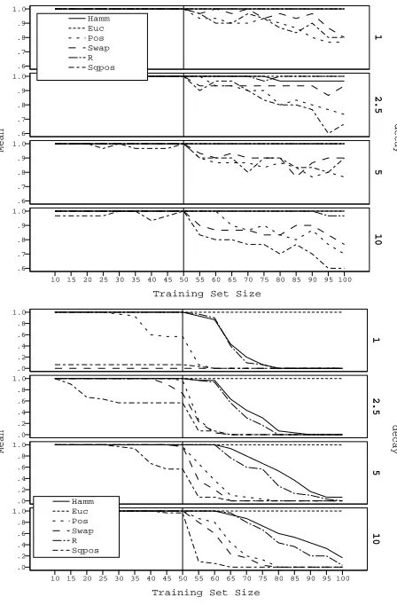
Figure 2 shows for each distance metric and decay factor, the proportion of matrices successfully inverted using the Gauss-Jordan algorithm (top) and via Cholesky factorisa-tion (bottom) asN increases. N is the number of samples in the training set, or equivalently, the size of the RBF net-work (the surrogate model). On each plot a vertical line shows the point at which training set moves from the initial random population, to also containing evolved solutions.

In each case there is a clear transition for most metrics aroundN≈50 - most notably for Pos, SqPos, and Swap.

For the Gauss-Jordan approach, increasing the “decay fac-tor”, so that the contribution of each RBF diminishes more rapidly with difference, has little effect. In contrast, using Cholesky factorisation it has a more dramatic effect, mak-ing the process more stable, although still not sufficiently so that one could consider it a practical approach.

We hypothesize that the cause of the instability is that distances between evolved solutions and their parents tend to be closer than distances between the randomly created initial population. This would lead to small values in the matrixAto be inverted. Given the length of the sequences considered, this could lead to numerical instability from di-vision by very small numbers, which would be partially ame-liorated by increasing the decay factor. Figure 3 shows this change in the minimum distance between samples in the training set as a function of its size N, and oﬀers evidence to support this hypothesis.

We experimented with using a range of multipliers and logarithms in order to try and reduce the numerical insta-bility, but these were only partially successful. To reduce the likelihood of coding errors or the impact of different im-plementations, we also tried three different implementations for each method taken from ‘a mixture of academic sites and highly voted answers on stackexchange.com. This had lit-tle or no effect. By contrast, directly solving the system of simultaneous equations via Gaussian elimination, although marginally less accurate, proved notably more stable.

4.2 Accuracy of Absolute Predicted Value

The errors in the absolute predicted values were often con-siderable. Figure 4 illustrates this by plotting the number of test set samples predicted to have (impossible) negative cost as the training set size (N) and the decay factor for the RBFs was varied. Although harder to measure, it seems like that a similar number may have had dramatically over-predicted costs. Figure 4 shows that:

• The number of samples incorrectly predicted to have negative costs rises withN when the RBF network is trying to model the cost surface (landscape) for most distance metrics, especially for Pos and SqPos.

• Increasing the decay factord, and hence the rate at which the contribution of each RBF falls oﬀ with dis-tance, reduces the number of negative predictions in most cases.

(5)

Mean 1.0 .9 .8 .7 .6 1.0 .9 .8 .7 .6 1.0 .9 .8 .7 .6

Training Set Size

100 95 90 85 80 75 70 65 60 55 50 45 40 35 30 25 20 15 10 1.0 .9 .8 .7 .6 decay 1 2.5 5 1 0 Sqpos R Swap Pos Euc Hamm Mean 1.0 .8 .6 .4 .2 .0 1.0 .8 .6 .4 .2 .0 1.0 .8 .6 .4 .2 .0

Training Set Size

[image:5.595.318.556.50.218.2]

100 95 90 85 80 75 70 65 60 55 50 45 40 35 30 25 20 15 10 1.0 .8 .6 .4 .2 .0 decay 1 2.5 5 1 0 Sqpos R Swap Pos Euc Hamm

Figure 2: Proportion of matrices successfully in-verted as a function of size (N) and distance met-ric using Gauss-Jordan (top) and Cholesky (bottom) methods. Vertical reference line shows the point at which the training set contains evolved solutions as well as the initial randomised population.

A simple thought experiment illustrates a likely cause for the negative predictions. Imagine a single dimension with two closely spaced RBFs based on observed samples. If the sam-ples have similar costs, then the surface can be modelled by assigning a nearly equal (roughly half-height) positive weight to each so that their summed contributions reach the desired costs at the known samples. Since both weights are positive, all points will have positive predicted costs. However, if the costs are very different, then the slope of the summed con-tributions needs to be sharply negative between them. The only way this can be achieved when both RBFs have large widths is if the weight of the RBF based on the higher-cost sample is large and positive, and the other is negative. Since the contributions of the RBFs to the summed cost prediction fall off with the square of the distance, this means that at some stage the prediction surface becomes negative. More-over, the extent to which this happens will reflect the extent to which nearby pairs of samples have different costs - in other words the ruggedness of the landscape.

In practice, we curtailed the predictions to a lower bound of zero (since costs cannot be negative). Figure 5 shows the variation of mean MSE with the size of the RBF network

[image:5.595.62.286.52.393.2]

N 100 95 90 85 80 75 70 65 60 55 50 45 40 35 30 25 20 15 10 Mean (Error bars 95% Confidence interval) 1.0 0.8 0.6 0.4 0.2 0.0 Sq.Pos R Swap Pos Euclidean Hamming

Figure 3: Change in minimum pairwise distance be-tween samples in training set as a function of N. Plot shows mean (over all instances) value for each metric with error bars for 95% conﬁdence intervals.

Mean 200 150 100 50 0 200 150 100 50 0 200 150 100 50 0

Training Set Size: N

100 95 90 85 80 75 70 65 60 55 50 45 40 35 30 25 20 15 10 200 150 100 50 0 d 1 2.5 5 1 0 Ens SqPos R Swap Pos Euc Hamm

Figure 4: Line plot for each distance metric, and the ensemble, of the mean number of test samples predicted to have negative cost, as a function of N

and d. Maximum possible values are 1000 -N.

for diﬀerent distance metrics, illustrated by the smallest, median, and largest, instances, which have lengths of 50, 517 and 1928 respectively. The same phase transition can be seen in the prediction accuracy as was noted in the nu-merical stability of the modelling process. To re-emphasise the implications of this point:

• At the start of a run of surrogate-assisted optimisation, when the models are built from a few random samples, the prediction error over the test set is relatively small.

[image:5.595.322.539.287.505.2]

(6)

to include evolved solutions the observed prediction er-ror actually increases.

Notably, the values of MSE are consistently higher for the problem instances with lower sequence lengths, hence smaller search spaces to be modelled. This may be because in the larger spaces more points are far from each other, and so the results are eﬀectively regressing to the mean.

Mean

100

10

1 0.0E0

decay

1 10

100

10

1 0.0E0

Training Set Size

100

95

90

85

80

75

70

65

60

55

50

45

40

35

30

25

20

15

10

100

10

1 0.0E0

100

95

90

85

80

75

70

65

60

55

50

45

40

35

30

25

20

15

10

Sequence Length

50

517

1928

Dumb Ens Sqpos R

Swap Pos Euc Hamm

Figure 5: Three typical examples of how the abso-lute prediction error (MSE) changes with network size and decay factor for diﬀerent distance metrics.

Further analysis shows that prior to the phase transition at N = 50 there is little difference between the metrics. Space precludes full reporting of all the possible tests. Tak-ing typical values of d = 1 and N = 25, Friedman’s non-parametric test rejects the null hypothesis that the mean MSE for each metric is identical with more than 95% con-fidence. However, paired sample t-tests between the results for each metric and the “dumb” predictor show that the only significantly different group is the Swap metric - which has worse MSE results (t=1.922, df=29, significance = 0.064).

For a typical value after the phase transition (N=75), we see a similar pattern except that now it is the Pos metric which has signiﬁcantly higher MSE values (t=1.896, df=29, signiﬁcance = 0.064).

Taken at face value, these results suggest a risk that sur-rogate models are no more accurate at predicting absolute ﬁtness values than a constant mean prediction, and often

worse once evolved points are used for training. The next experiments investigate whether the surrogate models accu-rately predict solution ranking.

4.3 Accuracy of Ranked Predicted Value

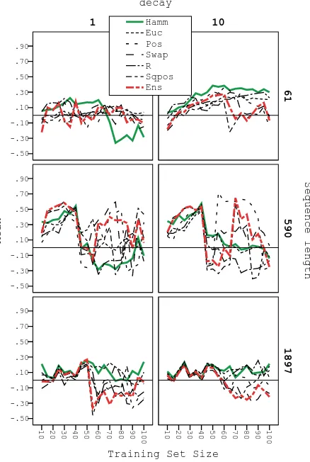
Figures 6 and 7 illustrate the behaviour ofρselandρ∼sel

asdandN are varied for three typical examples of different sizes. The phase transition effect is still present with these rank metrics, but much less marked than it was for MSE of absolute fitness.

Statistical analysis shows that the effect ofdis not signif-icant forρsel orρ∼sel. Although there is considerable vari-ation withN, it is somewhat random in nature so a linear model has no predictive power. Averaged over all runs, both measures are positive for each distance metric. If an RBF Network had no predictive value, the value for each measure would be 0.0, so we used a 1-sample Wilcoxon signed rank test to compare the median values against this constant. With 95% confidence the null hypothesis (no difference) can be rejected for the Euc, Pos and R distance metrics with

ρsel and for all metrics withρ∼sel.

Overall these results suggest that although the estimated cost surfaces may be distorted relative to the true cost sur-faces, they are preserving at least a partial rank-ordering of solutions, which is the critical measure for rank-based selec-tion methods such as tournament or truncaselec-tion selecselec-tion in evolutionary algorithms.

4.4 Optimisation Performance

In the light of previous results, we compared the original GA results to those from an algorithm using a single surro-gate model based on the Hamming distance (SMOHamm), and one using all six distance metrics and then taking an average to get an ensemble prediction (SMOEns).

In terms of effectiveness, the cost of the best solution found was lower for SMOHamm than for GA on 11 of the 32 instances, the same on 4 and higher on 17. The mean difference was 0.034% and a paired samples t-test showed the effect was not statistically significant. In terms of ef-ficiency, the time taken to find the best solution for that run was lower for SMOHamm than GA on 22 instances, the same on 2 and greater on 8. Using a paired samples one-tailed t-test showed that with more than 98% confidence we could reject the null hypotheses. Therefore we can conclude that using the Surrogate Model pre-selection phase statis-tically significantly decreased the number of solutions fully evaluated before the best solution was found.

A similar comparison of effectiveness and efficiency for SMOEns vs. GA yielded similar results. The the cost of the best solution found was the same on 4 instances and SMOEns and GA each found cheaper solutions on 14 in-stances. SMOEns found its best solution faster on 20 of the instances, slower on 8 of the instances and in the same time on 4. The one-tailed paired samples t-test on speed between SMOEns and GA allowed us to reject the null hypothesis (no difference) with 96% confidence.

Analysis showed neither efficiency nor effectiveness dif-fered significantly between the two surrogate-assisted algo-rithms.

5. CONCLUSIONS

(7)

Mean .40

.20

.00

-.20

decay

10 1

.40

.20

.00

-.20

Training Set Size

100

90

80

70

60

50

40

30

20

10

.40

.20

.00

-.20

100

90

80

70

60

50

40

30

20

10

Sequence length

59

551

1928

[image:7.595.63.275.61.390.2]

Ens Sqpos R Swap Pos Euc Hamm

Figure 6: Examples of small, medium and large in-stances showing how theρselmeasure of ranking pre-dictions changes with network size and decay factor for diﬀerent distance metrics.

approach for large combinatorial ordering problems with costly evaluation functions. We also hypothesized that pro-ducing several models using diﬀerent distance metrics in the RBF kernels would naturally induce a diverse set of models, and so produce an ensemble with a low prediction error.

What we discovered in fact was rather diﬀerent - although perhaps more useful as a source of guidance for practitioners:

• Numerical instability was a serious issue for the two most common methods of tuning the RBF weights, even when the matrices describing the linear system were positive definite. The observed occurrence of instability increased significantly once the algorithms started to included sample points create by evolution as well as the initial random population. Zaefferer et al. noted problems with the Gauss-Jordan approach [7]. Here, we observed even more significant problems with Cholesky decomposition. We have offered an ex-planation in terms of the increasing presence of sam-ples very close to each other, which is supported by experimental evidence. Clearly, the message here is that when deploying RBF networks as surrogate mod-els of permutation landscapes, it is necessary to check that the validity of the partial results involved in the

Mean

.90

.70

.50

.30

.10

-.10

-.30

-.50

decay

10 1

.90

.70

.50

.30

.10

-.10

-.30

-.50

Training Set Size

100

90

80

70

60

50

40

30

20

10

.90

.70

.50

.30

.10

-.10

-.30

-.50

100

90

80

70

60

50

40

30

20

10

Sequence length

61

590

1897

Ens Sqpos R Swap Pos Euc Hamm

Figure 7: Examples of small, medium and large in-stances showing how the ρ∼sel measure of ranking predictions changes with network size and decay fac-tor for diﬀerent distance metrics.

process rather than assuming correctness, even with established code libraries. Our recommendation in the case of costly, or diﬃcult to reproduce, ﬁtness evalu-ations would be to employ several approaches in par-allel, as is common practice in other mission-critical software design.

• Even when numerical stability was not an issue, we still observed an effect of increasingly poor prediction accuracy (for example, negative costs) in some cases. Again we offer an explanation in terms of the distribu-tion of samples and the ruggedness of the landscape. We note that Kim et al. reported that the accuracy of their RBF models was significantly affected by the RBF widths [5], and we observed some similar affects. This suggests that possibly an automatic tuning pro-cedure fordcould be devised by minimising the occur-rence of negative predictions, and we will explore this in future work.

[image:7.595.328.547.62.388.2]

(8)

building. Although it might not seem wise to discard hard-earned information, our results suggest that it might be preferable to take into account proximity to other samples: either in selecting bases; or in locally tuning their widths rather than using a global value as previous authors have done.

• Given the above observations about occasional high er-ror values, it is unsurprising that an ensemble of RBF networks using all of the distance metrics does not pre-dict absolute cost values well. It remains for future work to see if a more selective approach to ensemble creation might pay dividends.

• The results for the measures comparing the rankings of solutions according to predicted or actual costs were more positive. This suggests that even given the eﬀects and phase transitions noted above, the prediction land-scapes do preserve at least partial rank ordering.

• In the context of evolutionary optimisation, results showed that although the surrogate-assisted optimisa-tion did not statistically improve the best discovered solutions, itdidallow those solutions to be found using significantly fewer calls to the true cost function. In other words, although the RBF Network model might not have sufficient fidelity to fine-tune search, they still contain enough information to allow the search process to more rapidly home-in on areas likely to contain good quality solutions.

In order to place these results in context, we return to the starting point of this paper: the successes of meta-heuristic search algorithms have lead to them being increasingly ap-plied to more and more complex real-world problems with costly fitness evaluations. Surrogate-assisted optimisation has had many notable successes in the continuous domain, and current practice has been much influenced by experi-ence gained from applications. A few recent papers on small scale “academic” problems have suggested that these ben-efits might be carried over to permutation representations, and this paper makes a contribution to the understanding needed to achieve those gains.

6. ACKNOWLEDGMENTS

The authors would like to thank oﬃcers of the UK Oﬃce for National Statistics for their insights and experience of Cell Suppression Problem.

7. REFERENCES

[1] Y. Jin. A comprehensive survey of ﬁtness approximation in evolutionary computation.Soft Computing, 9(1): 3–12, 2005

[2] D. R. Jones, M. Schonlau, and W. J. Welch. Eﬃcient global optimization of expensive black-box functions.

Journal of Global Optimization, 13(4):455–492, 1998.

[3] Y. Jin. Surrogate-assisted evolutionary computation: Recent advances and future challenges.Swarm and Evolutionary Computation, 1(2):61–70, June 2011. [4] A. Moraglio, Y. H. Kim, and Y. Yoon. Geometric

surrogate-based optimisation for permutation-based problems. InCompanion volume to the proceedings of GECCO 2011: the ACM-SIGEVO conference on Genetic and Evolutionary Computation, 2011. [5] Y.-H. Kim, A. Moraglio, A. Kattan, and Y. Yoon.

Geometric Generalisation of Surrogate Model-Based Optimisation to Combinatorial and Program Spaces.

Mathematical Problems in Engineering, 2014(1):1–10, 2014.

[6] M. Zaefferer, J. Stork, M. Friese, and A. Fischbach. Efficient global optimization for combinatorial problems. InProceedings of GECCO 2014, the 2014 Annual Conference on Genetic and Evolutionary Computation, pages 871–878. ACM Press, July 2014. [7] M. Zaefferer, J. Stork, and T. Bartz-Beielstein.

Distance measures for permutations in combinatorial eﬃcient global optimization. InProceedings of the 13th International Conference on Parallel Problem Solving from Nature. Springer, 2014.

[8] G. Brown, J. Wyatt, R. Harris, and X. Yao. Diversity creation methods: a survey and categorisation.

Information Fusion, 2005.

[9] J. Kelly, B. Golden, and A. Assad. Cell suppression: Disclosure protection for sensitive tabular data.

Networks, 22(4):397–417, 1992.

[10] A. Staggemeier, A. Clark, J. Smith, and J. Thompson. Improving our knowledge of metaheuristic approaches for the cell suppression problem. InProceedings of Joint UNECE/Eurostat work session on statistical data confidentiality, December 2007.

[11] J. Smith, A. Clark, and A. Staggemeier. A genetic approach to statistical disclosure control. In

Proceedings of GECCO 2009, the ACM-SIGEVO conference on Evolutionary Computation, pages 1625–1632. Springer, July 2009.

[12] J. Smith, A. Clark, A. Staggemeier, and M. Serpell. A genetic approach to statistical disclosure control.

IEEE Transactions on Evolutionary Computation, 16(3):431–441, June 2012.

[13] V. Campos, M. Laguna, and R. Mart˜o.