1
An Enhanced Linear Kalman Filter (EnLKF) algorithm for parameter estimation of nonlinear rational models
Quanmin Zhu1,3*, Dingli Yu2, Dongya Zhao3
1 Department of Engineering, Design and Mathematics, University of the West of England, Frenchay Campus, Coldharbour Lane, Bristol, BS16 1QY, UK, Email: [email protected]
2 Control Systems Research Group, School of Engineering, Liverpool John Moores University, Byrom Street, Liverpool, L3 3AF, UK, Email: [email protected]
3 Department of Chemical Industrial Equipment and Control Engineering, College of Chemical Engineering, China University of Petroleum, Qingdao, 266580, China, Email: [email protected]
* Corresponding author
Abstract: In this study an enhanced Kalman Filter formulation for linear in the parameters models with inherent correlated errors is proposed to build up a new framework for nonlinear rational model parameter estimation. The mechanism of Linear Kalman Filter (LKF) with point data processing is adopted to develop a new recursive algorithm. The novelty of the Enhanced Linear Kalman Filter (EnLKF in short and distinguished from Extended Kalman Filter (EKF)) is that it is not formulated from the routes of extended Kalman Filters (to approximate nonlinear models by linear approximation around operating points through Taylor expansion) and also it includes LKF as its subset while linear models have no correlated errors in regressor terms. No matter linear or nonlinear models in representing a system from measured data, it is very common to have correlated errors between measurement noise and regression terms, the EnLKF provides a general solution for unbiased model parameter estimation without extra cost to convert model structure. The associated convergence is analysed to provide a quantitative indicator for applications and reference for further research. Three simulated examples are selected to bench-test the performance of the algorithm. In addition, the style of conducting numerical simulation studies provides a user-friendly step by step procedure for the readers/users with interest in their ad hoc applications. It should be noted that this approach is fundamentally different from those using linearization to approximate nonlinear models and then conduct state/parameter estimate.
Keywords: Nonlinear rational models, NARMAX models, parameter estimation, Kalman Filter, recursive algorithms, data driven modelling, simulations.
1 Introduction
Most research and experiments in the fields of science, engineering and social studies have spent significant efforts to find rules from various complicated phenomena by observations, recorded data, logical derivations, and so on. The rules are normally summarised as concise and quantitative expressions or "models". In regarding to modelling of man-made systems and natural systems, there are two major routes, one from principles such as Newton’s second law for building up mass-spring-damper models, the other is measured data based model fitting such as well-known least squares algorithms.
2
without proper physical and/or meaningful explanations (except numerical relationship) of the variables and parameters of the system internals. With ever-increased computing power, the way to model complex and nonlinear systems is changing. However fast and efficient computational algorithms in principle of parsimony are always encouraged in research and applications. In the procedure of modelling from data, for a given model structure, “parameter estimation” is the next paramount important task to extract the parameters embedded in the model from measured data sequences.
The second background of the study is about the model structure --- nonlinear rational model. A critical issue associated with rational model identification (including model structure detection and parameter estimation) using least squares approaches is the inherent correlation error between dependent variable and some regression terms while the denominator polynomial of the rational model is multiplied with output to expand into a linear regression expression.
Accordingly the aim of the study is to take the critical issue into consideration to derive solutions while using LKF for recursive parameter estimation of the rational model set. The aim is justified by the following analyses.
1) Although rational model parameter estimation has achieved certain level of results in format of batch data processing, there has been no enough study on recursive algorithms except the sole paper (Zhu and Billings 1991). It is an acceptable and reasonable claim for this study that the other well-known recursive computational algorithms such as Kalman Filters, Bayesian estimation mechanism, and so on could be applicable after properly revised/extended from their standard formulations. It is generally accepted that recursive algorithms are particularly important for real time adaptive control and other real time systems (Chen and Zhao 2014).
2) To support justification 1, Kalman Filter is selected. It should be noted that the classical formulation must be revised to accommodate the correlated error problems in the parameter estimation, which is an inherent phenomenon in applying linear regression algorithms to such nonlinear models. The novelty of the proposed algorithm comes from the facts that it is not formulated following the routes of extended Kalman Filters (for nonlinear models) and also it enhances classical linear Kalman Filters (for linear models) to directly deal with nonlinear rational models parameter estimation. The new formulation is concise and meaningful with those involved variables.
3) It is the author’s believe, that many other researchers are reluctant to study the identification and control of rational model is because rational model has a denominator polynomial to make it a total nonlinear in both parameters (model identification) and inputs (control system design), which the analysis and design are much more challenging than polynomial models (Narendra and Parthasapathy 1990, Zhu, Wang, Zhao, Li, and Billings 2015). However rational model has the four basic algebra operations (addition, subtraction, multiplication, and division) to cover almost all types of model as its subsets. The justification for using the rational model is that it provides a very concise and parsimonious representation for complex non-linear systems and has excellent extrapolation properties. Hopefully this study provides another encouragement/stimulation in the research areas besides its technical contribution.
3
lay a foundation for the following development. In section 3, a new Enhanced Linear Kalman Filter (EnLKF) algorithm is developed and its convergence analysis is delivered as well. A few of remarks are presented to intemperate the characteristics of the EnLKF. In section 4, model validity test --- higher order correlation functions are explained for testing the following case studies. In section 5, three bench tests are conducted to demonstrate the EnLKF efficiency and effectiveness. In section 6, a brief conclusion is drawn to summarise the results and to invite colleagues to provide counter examples and comments on the weakness of EnLKF to improve the new algorithm.
Throughout this study, operators E
* and * denote expectation and Euclidian norm respectively. Idenotes an identify matrix of appropriate dimensions.2 Rational model and parameter estimation 2.1 Rational model
Mathematically a general discrete time non-linear dynamic rational model is defined as
( 1),... ( ), ( 1),... ( ), ( 1),... ( )
( ) ˆ
( ) ( ) ( ) ( ) ( )
( ) ( 1),... ( ), ( 1),... ( ), ( 1),... ( )
nu ny ne
du dy de
a u t u t n y t y t n e t e t n
a t
y t y t e t e t e t
b t b u t u t n y t y t n e t e t n
(1)
where y t( )R and y tˆ( )Rare the measured and model output respectively, u t( )Ris the input, e t( )R is a noise sequence to represent the model error, which is defined as unobservable independent and identically distributed (iid) with zero mean and finite variance
2
e
, and t (= 1, 2, …) is the discrete time index. Generally the numerator a(t) and denominator
b(t) (b t( )0) are smooth (continuously differentiable) linear or non-linear functions of past inputs, outputs, and errors, and can be expressed in terms of polynomials
1
1
( ) ( )
( ) ( )
num
nj nj
j den
dj dj
j
a t p t
b t p t
(2)The regression terms pnj( )t and pdj( )t are the products of past inputs, outputs, and errors,
such as u t( 1) (y t3), u t( 1) (e t2), 2 ( 1)
y t , and nj and dj are the associated parameters. The task of the estimation, for a given model structure, is to estimate the associated parameters from the measured inputs and outputs.
Several remarks relating to the characteristics and identification of the rational model of (1) are noted below:
4
2) The model is non-linear in both the parameters and the regression terms. This is induced by the denominator polynomial. Such nonlinear model has been referred as total nonlinear model recently (Zhu, Wang, Zhao, Li, and Billings 2015).
3) The model can be much more concise than a polynomial expansion, for example
2 4
2
( 1)
( ) ( 1) 1 ( 1) ( 1)
1 ( 1)
u t
y t u t y t y t
y t
(3)
4) The model can produce large deviations in the output, for example
1 ( )
1 ( 1)
y t
u t
(4)
When u(t-1) approaches –1, the model output response will be extremely large. Hence the power to capture quick and large changes is gained by introducing the denominator polynomial.
5) Rational models have been gradually adopted in various applications of non-linear system modelling and control (Ford, Titterington, and Kitsos 1989, Ponton 1993, Correay and Aguirre 2000, Knežević-stevanović et al 2014, Gómez-Salas, Wang, and Zhu 2015), particularly the importance of modelling of chemical kinetics has increased sharply as a consequence of the applicability of modelling of catalytic reactions (Dimitrov and Kamenski 1991, Kamenski and Dimitrov1993). Rational models are not only alternative expressions in approximating a wide range of data set in chemical engineering, but also are class mechanistic models, which most previous experience or theoretical considerations had not put forwarded (Dimitrov and Kamenski 1991).
6) Many neuro-fuzzy systems have been expressed as non-linear rational models (Wang 1994). For example fuzzy systems with centre defuzzifier, product inference rule, singleton fuzzifier, and Gaussian membership function. The normalised radial basis function network is also a type of rational model. When the centres and widths are estimated this becomes a typical rational model parameter estimation problem (Zhu 2005).
7) Additionally the non-linear rational model can be described in a neural network structure (Zhu 2003). Here the rational model neural network is structured with an input layer of regression terms pnj( )t and pdj(t), a hidden layer of a(t) and b(t) with linear activation
functions, an output layer of y(t) with a ratio activation function. The activation function at the output layer is the division operation of the numerator polynomial divided by the denominator polynomial. It has been observed that Leung and Haykin (1993) presented a rational function neural network. The shortcomings compared with Zhu’s results (2003) are that Leung and Haykin's network does not have a generalised rational model structure and correlated errors are not accommodated. Hence Leung and Haykin's parameter estimation algorithm cannot provide unbiased estimates with noise corrupted data, and is essentially a special implementation of the procedure of Zhu (2003) in the case of noise free data.
5
recently a work (Zhu, Wang, Zhao, Li, and Billings 2015) has contributed a review paper on rational (total) nonlinear dynamic system modelling, identification and control.
9) In regarding to control system design, so far there is no analytical approach to design rational model based control systems, even though rational models have been used as complex nonlinear plants in neural control systems (Narendra and Parthasapathy 1990) which are treated as black boxes, that is, the model structure and parameters are not referred for control system design analytically.
2.2 Parameter estimation with correlated errors in regression terms
For estimating rational model parameters, Billings and Zhu (1991) has proposed an extended least squares algorithm. In the two step procedure, 1) expand rational model into a linear in parameters expression and 2) then extend standard least squares algorithms with accommodating the estimate bias induced by correlated errors in regression variables, which are appeared from the model expression conversion. In the other word, the linear in the parameter expression is achieved at the expenses of inducing correlated errors.
Step 1: To obtain its linear in the parameters expression (Billings and Zhu 1991), multiplying numerator polynomial b(t) of rational model on both sides of (1) in conjunction with (2), then moving all the terms except Y t( ) y t p( ) d1( )t d1to the right hand side, it gives
2
1 2
1
1 2
( ) ( ) ( ) ( ) ( ) ( )
( ) ( ) ( ) ( ) ( )
( )
( ) ( ) ( ) ( )
( ) den
dj dj
j
num den
nj nj dj dj
j j
num den
nj nj dj dj d
j j
Y t a t y t p t b t e t
p t y t p t b t e t
a t
p t p t p t e t
b t
(5)
It should be noted that the second line of (5) represents from measured data and the third line
of (5) is an analytical expression as ( ) ( )
a t
b t is not measureable. The linear in the parameter
expression of (5) can be further expressed in terms of vector with measurable data.
( ) T( ) ( )
Y t t t (6)
where
1 2
1 2
( ) ( ) ( ) ( ) ( ) ( ) ( ) ( )
( ) ( ) ( )
( ) n d T n nnum d dden T
T T
n d n nnum d dden
t t p t p t y t p t y t p t
t b
t
t e t
(7)
Regarding to this study, assume d11, therefore
1
1 1 1 1
( )
( ) ( ) ( ) | ( ) ( ) ( )
( ) d
d d d
a t
Y t y t p t p t p t e t
b t
6
And
( )
( ) ( )
( ) e( )E t E b t e t E b t E t (9)
Provided e(t) has been reduced to an uncorrelated sequence as defined in (1).
Inspection of the regression model of (5), it has been studied (Billings and Zhu 1991) that all the denominator terms y t p t( ) dj( ) implicitly include a current noise e(t) which is highly correlated with ( )t , the model error, in (5). Accordingly this is the course of the bias using classical least squares algorithms for parameter estimation.
Step 2: A general rational model least square algorithm has been developed (Billings and Zhu 1991)
1
2 2
ˆ T T
e Y e
(10)
where e2 is the noise variance of rational model (1), which must be estimated in advance. Billings and Zhu (1991) and Zhu (2003, 2005) have proposed some iterative algorithms to estimate the variance while estimative the model parameters. The other notations in above estimator are explained below.
Parameter estimate vector
1 2
ˆ ˆ ˆ ˆ
ˆ ˆ ˆ T T
n d n nnum d dden
(11)
Regressor matrix
(1) (1) (1)( ) ( ) ( )
T T T
n d
n d
T T T
n d
N N N
(12)
Dependant vector
(1) ( )
TY Y Y N (13)
Denominator (without pd1( )t ) regressor matrix and cross product vector of denominator (without pd1( )t ) and pd1( )t
1 0
0 0
0 T Tpd
2
2
(1) (1)
( ) ( )
d dden
d dden
p p
p N p N
7
where N is the data length and pd1( )t data vector is defined as
1 1(1) 1( )
T
d d d
p p p N (15)
The estimator has been proved to have the following statistics (Billing and Zhu 1991). The estimate bias, in term of the 1st order statistical average, is
ˆ
( ) 0
Bias (16)
And the estimate co-variance, in terms of the 2nd order statistical average, is
1 1
2 2 2 2 2
ˆ
cov( ) e b T e e b T
(17)
where b2is the variance of denominator polynomial b(t).
3. Linear Kalman Filter (LKF) for parameter estimation
In this section classical Linear Kalman Filter (LKF) is briefly explained to lay a foundation for the development of Enhanced Linear Kalman Filter (EnLKF) algorithm. Then based on the error analysis of the rational model parameter estimation, EnLFK is derived to obtained unbiased estimates. Subsequently the EnLKF convergence conditions are analysed and remarks are given to explain the EnLKF characteristics.
3.1 Classical Linear Kalman Filter (LKF) for model parameter estimation
This section is referred from a well-known and widely used book (Ljung 1999), which the relevant algorithms have been included as standard tools in Matlab System Identification Toolbox.
For building up Kalman Filter based recursive parameter estimation framework, first consider a general linear in the parameter regression model of
( ) T( ) ( )
Y t t e t (18)
where Y t( )R1is the measured output,( )t Rnis the regression vector, which the specific form of ( )t depends on the structure of the polynomial model. Rn represents the true parameter vector, and e t( )R1is the measurement noise subject to iid.
In this study, Kalman filter is used to obtain ˆ(the estimate of ) from measured data. A pair of Kalman equations is generally given in the following form of
( ) ( 1) ( 1) (update model)
( ) ( ) ( ) ( ) (observation model)
n T
t I t w t
Y t t t e t
(19)
8
linear in the parameter recursive representation from rational model expansion (5) and the second equation is the original rational model (1).
Accordingly the recursive parameter estimation vector ˆ ( )t can be formulated as
1
ˆ
( ) ( ) ( ) ( 1) (measurement residual)
S( ) ( ) ( 1) ( ) (residual covaraince)
( ) ( 1) ( ) ( ) (optimal Kalman gain)
ˆ( ) ˆ( 1) ( ) ( ) (updated parameter estimate)
( ) ( ) ( ) ( 1)
T T
T
t Y t t t
t R t P t t
K t P t t S t
t t K t t
P t I K t t P t
Q (updated covaraince estimate)
(20)
3.2 Enhanced Linear Kalman Filter (EnLKF) for nonlinear rational model parameter estimation
From previous results (Billing and Zhu 1991) and the brief in Section 2, the correlated errors are exist in formation of ( )t T( )t , T( ) ( )t t , and ( ) ( )t Y t . Therefore, the first step in deriving the EnLKF is to condense the above five equations in (20) into two equations, that is parameter update equation and covariance update equation by eliminating ( ) t , K(t) and S(t) to make the three error contaminated terms explicitly expressed in the following equations.
1
1
ˆ( ) ˆ( 1) ( ) ( )
ˆ ( 1) ( 1) ( ) ( ) ( )
ˆ( 1) ( 1) ( ) ( ) ( ) ( ) (ˆ 1)
ˆ
( 1) ( ) ( ) ( ) ( ) ( 1)
ˆ ( 1)
( ) ( 1) ( )
( ) ( ) ( ) ( 1)
( 1) ( )( ) ( ) (
( 1) T T T T T
t t K t t
t P t t S t t
t P t t S t Y t t t
P t t Y t t t t
t
R t P t t
P t I K t t P t
P t t t t P
P t
1)
( )
( 1) ( )( ) ( ) ( 1)
( 1)
( ) ( 1) ( )
T T
t S t
P t t t t P t
P t Q
R t P t t
(21)
The expressions of (21) builds up a platform for EnLKF expansion.
Consequently in the second step of the derivation, the extended Kalman Filter algorithm is developed with removing the three induced error terms.
2 2
1
2
2
ˆ
( 1) ( ( ) ( ) ( ) ( )) ( ( ) ( ) ( ) ( )) ( 1))
ˆ( ) ˆ( 1)
( ( ) ( 1) ( ) ) ( ( ) ( 1) ( ))
( ( 1) ( )( ) ( ) ( 1)) ( ( 1) ( )( ) ( ) ( 1))
( ) ( 1)
( ( ) ( 1)
T T
e d e
T T
e
T T
e T
P t t Y t t p t t t t t t
t t
t P t t R t P t t
P t t t t P t P t t t t P t P t P t Q
t P t
2
( )t R) e( T( ) (t P t 1) ( )) t
9
where
1,
2
( ) 0 0 ( ) ( )
T n nnum
d dden
t p t p t
(23)
The other associated updates are summarised below.
1
2 2 2
2 2 2
ˆ
ˆ( ) ( ) ( 1)
ˆ( ) ( ) ( ) ˆ ( 1)
ˆ( )
ˆ( ) ( )
ˆ( ) 1
ˆ ( ) ˆ ( 1) ˆ ( )
1 ˆ
ˆ ( ) ˆ ( 1) ( )
T
n n
T
d d d
e e
b b
a t t t
b t p t t t
a t
e t y t
b t t
t t e t
t t
t t b t
t (24)
where notation xˆ for the estimate of x.
Remark 1: ENLKF (22) can be further meaningfully expressed as
ˆ
( 1) ( ) ( ) ( ) ( ) ( 1))
ˆ( ) ˆ( 1)
( ) ( 1) ( )
( 1) ( ) ( ) ( 1)
( ) ( 1)
( ) ( 1) ( )
T
T
T
T
P t t Y t t t t
t t
t P t t R
P t t t P t
P t P t Q
t P t t R
(25) where 2 1 2 2 2 ( ) ( ) ( ) ( ) ( ) ( ) ( ) ( ) ( ) ( ) ( ) ( )
( ) ( 1) ( ) ( ) ( 1) ( ) ( ) ( 1) ( )
( 1) ( ) ( ) ( 1) ( 1) ( ) ( ) ( 1) ( 1) ( ) ( ) ( 1)
e d
T T T
e
T T T
e
T T T
e
t Y t t Y t t p t
t t t t t t
t P t t t P t t t P t t
P t t t P t P t t t P t P t t t P t
10
( ) ( )
( ) ( )
( ) ( 1) ( )
( 1) ( )( ) ( ) ( 1)
T
T
T
E t Y t
E t t
E t P t t
E P t t t t P t
(27)
are the unbiased estimates, that is, the correlated error terms embedded have been removed. This property has been proved in batch least square algorithms for rational model parameter estimation (Billing and Zhu 1991). For comprehensive understanding of the properties it can be referred to a survey paper (Zhu, Wang, Zhao, Li, and Billings 2015).
Remark 2: Comparison with Extended Kalman Filter (EKF) and Linear Kalman Filter (LKF). The EnLKF is not formulated following the routes of EKF (for nonlinear models) and also it generalises classical linear Kalman Filters (for linear models) to directly deal with nonlinear rational models parameter estimation. The insight is explained below.
EKF
In principle, Kalman Filter is the optimal estimate for linear system models with additive independent white noise in both the transition and the measurement systems. In engineering, most systems are nonlinear, consequently EKF has been proposed for such nonlinear systems. The EKF adopts techniques from calculus, namely multivariate Taylor Series expansions, to linearize a model about a working point (Reif, Gunther, Yaz, and Unbehauen 1999). There has been some caution in using EKF, for example, optimal estimation, convergence, sensitivity to covariance matrix estimation. In general, EKF is highly computationally demanded due to the partial differentiation (Jacobian matrices) around approximation points. Although EKF can be used for rational model parameter estimation, it is at the expenses of the above mentioned problems (Extended Kalman Filter 2015).
LKF
Simply parameter estimates of rational model (while is converted into linear in the parameter expression, otherwise LKF cannot be applied to rational model parameter estimation directly) obtained using LKF do not converge to the true parameters due to the correlated errors between measured noise and those denominator regression terms. That is LKF is a biased estimator for nonlinear rational ration model parameters. As EnLKF is a general expression of LKF, it should be noted that EnLKF is also sensitive to the measured noise variance as the many other Kalman filters. EnLKF has not improved this critical property currently. In general, EnLKF shares similar convergent properties like LKF, an equivalent theorem on the convergence is proved in next subsection 3.3. The other equivalent properties between LKF and EnLKF should be properly addressed in the future studies.
11
Stoica 1989, Ljung 1999), recently developed (Ding et al 2015, 2016), and neuro-fuzzy (Shi et al, 2015, Ganesh and Thanushkodi 2015, Li et al 2015), the algorithms mainly deal with the issues of linear in the parameter estimation no matter of the model regression variables linear or nonlinear. However, they have weak requests on the knowledge of covariance matrices Q
and R, but many Kalman filter based algorithms are sensitive to the measurement noise variance, no exception for the EnLKF. It is possible for further research work to expand the EnLKF with more robustness to the variance variation.
3.3 Convergence analysis of EnLKF
In regarding to convergence analysis, this study takes an online convergence theorem (Rhudy and Gu 2013), which is proved with a modified well-known stochastic stability lemma (Reif, Gunther, Yaz, and, Unbehauen 1999), as a basis to extend for the EnLKF convergence analysis.
Linear Kalman filter convergence theorem (Rhudy and Gu 2013): Consider a linear stochastic systems of the following standard form
( ) ( ) ( 1) ( 1) (update model)
( ) ( ) ( ) ( ) (observation model)
x t F t x t w t y t H t x t v t
(28)
Where x t( )Rn is the state vector, y t( )Rm is the output vector, F t( )Rn n* and *
( ) m n
H t R are system matrices, ( 1) n
w t R and ( ) m
v t R are the process and measurement noise vectors that are zero mean, white, independent and have assumed covariance matrices
( 1)
Q t and R t( ) respectively. For this system, the corresponding classical Kalman Filter algorithm for the state estimate ˆ( )x t is formulated with standard set of equations (Rhudy and Gu 2013) Denote the estimation state estimation error as
ˆ ˆ
( ) ( ) ( ) (0) (0) (0)
e e
x t x t x t x x x (29)
Let the following assumptions hold.
1) The system matrix ( )F t is non-singular (invertible) for all t. 2) The assumed initial covariance is bounded.
2 1
(0) (0) (0) (0) (0)
T
e e e
x P x v x (30)
wherev(0)is a constant
3) The state error covariance matrix is bounded by the following inequality for all t. 2
1
( ) ( ) ( ) ( ) ( )
T
e e e
x t P t x t b t x t (31)
12
( 1) ( 1) ( 1)
( ) ( ) ( )
T
T
Q t E w t w t
R t E v t v t
(32)
Then the expected value of the estimation error is bounded in mean square with probability one by
1 1
2 2
0
0 1
(0) 1
( ) (0) 1 ( ) ( i 1) (1 ( )
( ) ( )
t t i
e e
i
i j
v
E x t E x i t t j
b t b t
(33)where the time varying parameters (t1), (t1)and b t( )are given by
min
1 min
( 1) ( ( ))
( 1) ( ( ))
( ) ( ( ))
t C t
t Tr C t
b t P t
(34)
where operators min( )P and Tr P( )denote the minimum eigenvalue and trace of matrix P
respectively, and
1
1 1
( ) ( 1) ( 1) T( ) ( ) ( ) ( 1) ( 1) ( 1) T( ) ( ) ( ) ( 1)
C t P t P t t R t t P t Q t P t t R t t P t (35)
Enhanced Linear Kalman filter convergence theorem: Consider a nonlinear stochastic systems represented by a rational model of (1) in conjunction with (2) and its Kalman filter equations of (19) in conjunction with (18), all the assumptions and conclusions for state estimation given in LKF (Rhudy and Gu 2013) are parallel equivalent with probability one for the parameter estimation of nonlinear rational models through EnLKF.
Proof: This includes proving both notation equivalency and formulation equivalency.
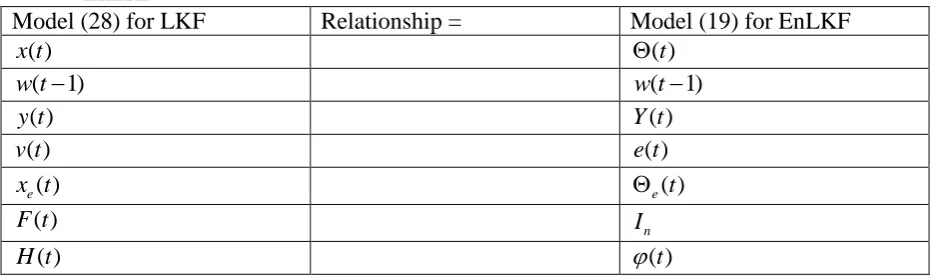
1) For notation equivalency, consider table 1 to compare the notations used in LFF and EnLKF
Model (28) for LKF Relationship = Model (19) for EnLKF
( )
x t ( )t
( 1)
w t w t( 1)
( )
y t Y t( )
( )
v t e t( )
( ) e
x t e( )t
( )
F t In
( )
[image:12.595.65.533.543.682.2]H t ( )t
Table 1 Notation equivalency between LKF and EnLKF
13
Formulation of (25) for LKF Relationship: = in terms of E[*]
Formulation of (21) for EnLKF
ˆ
( 1) ( ) ( ) ( ) ( ) ( 1) ˆ( ) ˆ( 1)
( ) ( 1) ( )
( 1) ( )( ) ( ) ( 1) ( ) ( 1)
( ) ( 1) ( )
T T
T T
P t t Y t t t t t t
R t P t t
P t t t t P t P t P t Q
R t P t t
ˆ
( 1) ( ) ( ) ( ) ( ) ( 1)) ˆ( ) ˆ( 1)
( ) ( 1) ( ) ( 1) ( )( ) ( ) ( 1) ( ) ( 1)
( ) ( 1) ( )
T
T
T T
P t t Y t t t t t t
t P t t R P t t t t P t P t P t Q
t P t t R
[image:13.595.71.263.390.529.2]
Table 2 Formulation equivalency between LKF and EnLKF
4 Model validation
There have been two correlation function based model validity tests, one is higher order correlation functions (Billings and Zhu 1994, 1995) and the other is the omni-directional correlation functions (Zhu, Zhang, and Longden 2007). It should be noticed that all validation methods developed based on nonlinear models have included all linear model validation as their simplified cases. However, the linear model based validation test methods can and often do fail when applied to nonlinear model validation.
In this study, to verify whether a model has been properly estimated, the higher order correlation function based tests are used as a terminating criterion. The two correlation functions are described below:
2 2 ___ 2 2 1 2 ___2 2 2
1 1 ___ 2 2 1 2 ___
2 2 2
1 1 ( ) ( ) ( ) ( ) ( ) ( ) ( ) ( ) ( ) ( ) N t N N t t N t u N N t t t t t t
t u t u
t u t u
(36)where is the delay, N is data length, and
1
___ ___
2 2 2 2
1 1 1 ( ) ( ) ( ) ( ) 1 1 ( ) ( ) N t N N t k
t y t t t
N
u u t t
N N
(37)Where y t( ) and u t( )are the measured output and input sequences respectively, and ˆ
( )t y t( ) y t( )
14
2
2
0 0
( ) 0 ( ) 0
u
k
otherwise
(38)
the estimated parameters are considered to be unbiased. In practice the 95% confidence limits, about 1.96/ N , are used as the confidence intervals.
Upon the parameters associated with the polynomials a(t) and b(t) having been estimated, the explicit output estimate y(t) can be determined and hence the residual ( )t . Therefore, the model validation procedure is still applicable to the developed algorithm.
5 Simulation studies
First of all, two simulated nonlinear rational model examples were selected to conduct bench tests of the EnLKF and compare with LKF. To generate the data for model parameter estimation, selected input u t( ) unif( 1,1) , a uniformly distributed random sequence with zero mean and variance of 0.33 (equivalently with an amplitude range of 1) and noise
(0) (0, 0.01)
e N , an uncorrelated Gaussian sequence with zero mean and variance of 0.01, which the input u(t) and the error e(t) were mutually independent in all cases. For each tested model, N = 1000 output data were generated with input and error stimulation through the model. The other initial setups included covariance matrix P(0) 10000* I, parameter vector
(0) unif( 1,1)
randomly selected without priori information, and e2(0)0for the
simulations required to estimate the measurement noise variance.
The first example was a simple noise free non-linear rational model. The purpose of testing this simple example is to investigate whether the parameter estimates are unbiased in the noise free case by both LKF and EnLKF. Further this demonstrates the feasibility to convert rational model into linear regression expression for parameter estimation.
The second example was designed for the test of estimating model parameters from noise corrupted data. This demonstrates the necessity to revise classical linear approaches to accommodate the expenses or extra problems induced at converting nonlinear in parameter models into linear regression expressions.
Finally, to demonstrate practical application of the theoretic results presented in the study, the third example, a propylene catalytic oxidation process model is selected, which is frequently operated in chemical engineering.
Example one: A simple noise free non-linear rational model was considered as below
2 2
0.3 ( 1) ( 2) 0.7 ( 1)
( )
1 ( 1) ( 1)
y t y t u t
y t
y t u t
(39)
For estimating the model parameters by Kalman Filters, expand model of (39) of its linear in the parameters expression below.
2 2
( ) 0.3 ( 1) ( 2) 0.7 ( 1) ( ) ( 1) ( ) ( 1)
15
where Y t( ) y t( )
Table 3 shows the estimates obtained by both LKF and EnLKF against true model parameters. Both filters generate unbiased estimates in noise free case.
Associated regression terms
LKF estimates EnLKF estimates True parameters
1( ) ( 1) ( 2)
n
p t y t y t 0.3 0.3 0.3
) 1 ( ) (
2 t ut
pn 0.7 0.7 0.7
1 ) ( 1 t
pd 1.0 1.0 1.0
) 1 ( )
( 2
2 t y t
pd 1.0 1.0 1.0
) 1 ( )
( 2
3 t u t
pd 1.0 1.0 1.0
Table 3 Estimates for Example 1
Example two: A non-linear rational model with uncorrelated noise
2 2
0.3 ( 1) ( 2) 0.7 ( 1)
( ) ( )
1 ( 1) ( 1)
y t y t u t
y t e t
y t u t
(41)
For estimating the model parameters by Kalman Filters, expand model of (41) of its linear in the parameters expression below.
2 2
2 2
( ) 0.3 ( 1) ( 2) 0.7 ( 1) ( ) ( 1) ( ) ( 1) ( ) ( )
0.3 ( 1) * ( 2) 0.7 ( 1) ( ) ( 1) ( ) ( 1) ( )
Y t y t y t u t y t y t y t u t b t e t y t y t u t y t y t y t u t t
(42)
where Y t( ) y t( )
NB: y(t) included in the denominator regression terms, which induces correlated errors with measured noise.
The test of the example was designed with two separate experiments
1) With estimate error covariance matrix Q108I and measurement noise variance
0.01
R .
2) With 8
10
Q Iand guessed R.
Table 4 shows the estimates obtained by both LKF and EnLKF with pre-known Q and R
against true model parameters.
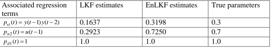
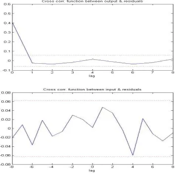
The model validation tests of EnLKF are shown in Fig. 1.
Associated regression terms
LKF estimates EnLKF estimates True parameters
1( ) ( 1) ( 2)
n
p t y t y t 0.1637 0.3198 0.3
) 1 ( ) (
2 t ut
pn 0.2923 0.7250 0.7
1 ) ( 1 t
[image:15.595.68.478.142.253.2] [image:15.595.68.512.679.757.2]16
) 1 ( )
( 2
2 t y t
pd -2.0516 1.1413 1.0
) 1 ( )
( 2
3 t u t
[image:16.595.73.506.70.108.2]pd -0.3137 1.0866 1.0
Table 4 Estimates with known R=0.01 for Example 2
It can be observed that classical linear Kalman filter cannot be used for rational model parameter estimation with noise contaminated measurements even though it work for noise free cases as shown in example one.
Table 5 shows the estimates obtained by EnLKF with two guessed R= 0.005 and 0.02 against true model parameters. Obviously none of them has acceptable estimates, which indicates the estimator, like the other Kalman filters, is very sensitive to the measured noise variance. Accordingly, users should be careful in applications.
Associated regression terms
EnLKF estimates,
R=0.005
EnLKF estimates
R=0.02
True parameters
1( ) ( 1) ( 2)
n
p t y t y t 0.1739 -0.3792 0.3
) 1 ( ) (
2 t ut
pn 0.4061 -1.1198 0.7
1 ) ( 1 t
pd 1.0 1.0 1.0
) 1 ( )
( 2
2 t y t
pd -1.2781 -11.0901 1.0
) 1 ( )
( 2
3 t u t
[image:16.595.70.506.273.383.2]pd 0.0486 -5.0865 1.0
Table 5 Estimates with guessed R for Example 2
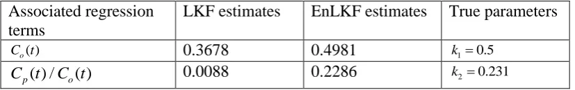
Example three: To illustrate application of the EnLKF algorithm for practical problems, a propylene catalytic oxidation process is selected, which is frequently operated in chemical engineering. The model (Dimitrov and Kamenski 1991) is given as below.
0.5 1
0.5 2
( ) ( )
( ) ( )
( ) ( )
o P
o P
k C t C t
r t e t
C t k C t
(43)
where two inputs CO(t) and CP(t) are the oxygen and propylene concentrations in mmol 1
-1
at time instant t respectively, output r(t) is the rate of disappearance of propylene in mmol
1
(g,s) , and measurement noise ( )e t is normally distributed subject to iid. k1 and k2 are the associated weights.
To use the EnLKF algorithm, the original model of (43) was normalised as
1
2 0.5
( )
( ) ( )
( ) 1
( ) P
P o
k C t
r t e t
C t k
C t
(44)
To prepare the simulation studies, the parameters were setup with k1 = 0.5 and k2 = 0.231, the two inputs were setup with independently uniformly distributed sequences,
( ), ( ) (1,3)
o p
17
with Q108I and the measurement noise variance R0.01. The same as the first two examples, the data length of the third example was fixed with 1000 points.
Table 6 shows the estimates obtained by both LKF and EnLKF against true model parameters. Obviously LKF is not applicable even for such simple practical case.
Associated regression terms
LKF estimates EnLKF estimates True parameters
( )
o
C t 0.3678 0.4981 k10.5
( ) / ( )
p o
[image:17.595.65.479.185.250.2]C t C t 0.0088 0.2286 k20.231
Table 6 Estimates for Example 3
In brief summary, this simple case study has illustrated a procedure to deal with practical problems. Especially model normalisation could be frequently used to transform various practical rational systems into proper formulisation for the application of the EnLKF algorithm. This study also indicates again that ordinary LKF is not applicable for the parameter estimation of nonlinear rational models.
6. Conclusions
This study represents a further advancement on nonlinear rational model identification. More importantly the study confirms again the author’s research hypothesis that many efficient methodologies/algorithms developed from linear models can be efficiently applied to deal with nonlinear model based analysis and design after properly changing the model expressions (NB, this is not linear approximation, the expression change has nothing in change of the model properties/characteristics. A generally parsimonious three step procedure developed from the author’s work is 1) convert underlying nonlinear model into a proper prototype to enable linear approaches basically applicable in structure, 2) identify the problems induced from the model conversion, and 3) then modify the linear ones to accommodate the problems induced from the model conversion. As another testimony of the research methodology, this study follows the procedure of 1) express nonlinear rational model into linear in parameters expression, 2) identify the inherent correlation errors between measurement noise variable and regressor terms, 3) revise LKF to accommodate the accumulated estimation errors. It should be noted that linear approximation is popular and widely used, but it gives approximation errors and creates largely computational complexity and demand due to the partial differentiation (Jacobian matrix, maybe plus Hessian matrix) around approximation points. This study is fundamentally different in treating nonlinear models for parameter estimation. Hopefully it can promote the less attended research methodology in dealing nonlinear system identification and control with linear approaches.
Last, but not least, it should be pointed out that the EnLKF has the same problem as many others, that is, sensitive to the measured noise variance. It is hoped to receive counter examples and comments on the weakness of the EnLKF, therefore to strengthen the applicability of the EnLKF tool box.
18
This work is partially supported by the National Nature Science Foundation of China under Grants 61273188 and 61473312, and Taishan Scholar Construction Engineering Special Funding, Shandong, China. Finally the authors are grateful to the editors and the anonymous reviewers for their helpful comments and constructive suggestions with regard to the revision of the paper.
References
Billings, S.A., Nonlinear System Identification: NARMAX Methods in the time, frequency, and spatio-temporal domains, Wiley, John & Sons, Chichester, West Sussex, 2013.
Billings, S.A. and Zhu, Q.M., Rational model identification using extended least squares algorithm, Int. J. Control, Vol. 54, pp. 529-546, 1991; Nonlinear model validation using correlation tests, ibid., Vol. 60, pp. 1107-1120, 1994; Model validation tests for multivariable nonlinear models including neural networks, ibid., Vol. 62, pp. 749-766, 1995.
Chen, H.F. and Zhao, W.X., Recursive identification and parameter estimation, CRC Press, Taylor & Francis, Singapore, 2014.
Correa, M.V. and Aguirre, L.A.,Modeling chaotic dynamics with discrete nonlinear rational models, Int. J. of Bifurcation and Chaos, Vol. 10, No. 5, pp.1019-1032, 2000.
Dimitrov, S.D. and Kamenski, D.I., A parameter estimation method for rational functions, Computers and Chemical Engineering, Vol. 15, pp. 657-662, 1991.
Ding, F., Wang, Y., and Ding, J., Recursive least squares parameter identification algorithms for systems with colored noise using the filtering technique and the auxilary model. Digital Signal Processing, Vol. 37, pp. 100-108, 2015.
Ding, F., Wang, X., Chen, Q., and Xiao, Y., Recursive least squares parameter estimation for a class of output nonlinear systems based on the model decomposition. Circuits, Systems, and Signal Processing, Vol. 35, 2016, doi: 10.1007/s00034-015-0190-6.
Extended Kalman Filter,Wikipedia [online],5 June 2015, Available from:
https://en.wikipedia.org/wiki/Extended_Kalman_filter, [Accessed 23 June 2015].
Ford, I., Titterington, D.M., and Kitsos, C.P., Recent advances in non-linear experimental design, Technometrics, Vol. 31, pp. 49-60, 1989.
Ganesh, M. K. S., & Thanushkodi, K., An efficient software cost Estimation technique using fuzzy logic with the aid of optimization algorithm. International Journal of Innovative Computing, Information and Control, Vol. 11, No. 2, pp. 587-597, 2015
Gómez-Salas, F., Wang, Y.J. and Zhu, Q.M., Design of a discrete tracking controller for a magnetic levitation system: a nonlinear rational model approach, Mathematical Problems in Engineering, Hindawi,Vol. 2015, Article ID 360783, 2015.
19
Knežević-stevanović, A. N., Babić, G.M., Kijevčanin, M.J., Šerbanović, S.P., and Grozdanić, D.K. Liquid mixture viscosities correlation with rational models, J. Serb. Chem. Soc. Vol. 79, No. 3, pp. 341–344, 2014.
Leung, H. and Haykin, S., Rational function neural network, Neural Computation, Vol. 5, pp. 928-938, 1993.
Li, F., Wu, L., Shi, P., & Lim, C.C., State estimation and sliding mode control for semi-Markovian jump systems with mismatched uncertainties. Automatica, Vol. 51, pp. 385-393, 2015.
Ljung, L., System Identification: Theory for the User, Prentice Hall PTR, Upper Saddle River, NJ, 1999.
Narendra, K.S. and Parthasapathy, K., Identification and control of dynamical systems using neural networks, IEEE Transactions on Neural Networks, Vol. 1, pp. 4-27, 1990.
Ponton, J.W., The use of multivariable rational functions for non-linear data presentation and classification, Computers and Chemical Engineering, Vol. 17, pp.1047-1052, 1993.
Proll, T. and Karim, M.N., Model predictive PH control using real time NARX approach, AIChe J., Vol. 40, pp. 269-282, 1994.
Reif, K., Gunther, S, Yaz, E., and Unbehauen, R., Stochastic stability of the discrete-time Extended Kalman Filter, IEEE Transactions on Automatic Control, Vol. 44, No. 4, pp. 714-728, 1999
Rhudy, M.B. and Gu, Y., Online stochastic convergence analysis of the Kalman Filter, International Journal of Stochastic Analysis, Volume 2013, Article ID 240295, 9 pages, Hindawi Publishing Corporation, available at http://dx.doi.org/10.1155/2013/240295
[Accessed 26 June 2015].
Shi, P., Zhang, Y., Chadli, M., and Agarwal, R. K., Mixed H-Infinity and Passive Filtering for Discrete Fuzzy Neural Networks With Stochastic Jumps and Time Delays, IEEE Transactions on Neural Networks and Learning Systems, Vol. PP, Issue 99, pp 1-7, 2015.
Soderstrom, T. and Stoica, P. System identification, Prentice Hall International, Hemel Hempstead, 1989.
Wang, L.X, Adaptive fuzzy systems and control, Prentice Hall, Englewood Cliffs, NJ, 1994.
Zhu, Q.M. and Billings, S.A, Recursive parameter estimation for nonlinear rational models, J. Sys. Engineering, Vol. 1, pp. 63-67, 1991; Parameter estimation for stochastic nonlinear models, Int. J. Control, Vol. 57, pp. 309-333, 1993.
Zhu, Q.M., A back propagation algorithm to estimate the parameters of nonlinear dynamic rational models, Applied Mathematical Modelling, Vol. 27, pp. 169-187, 2003.
20
Zhu, Q.M., Zhang, L.F., and Longden, A., Development of omni-directional correlation functions for nonlinear model validation, Vol. 43, pp. 1519-1531, Automatica, 2007.
[image:20.595.101.458.199.551.2]Zhu, Q.M., Wang, Y.J., Zhao, D.Y., Li, S.Y., and Billings, S.A., Review of rational (total) nonlinear dynamic system modelling, identification and control, Int. J. of Systems Science, V46, N12, pp. 122-133, 2015.