A Discrete Robust Adaptive Iterative Learning Control for a Class of Nonlinear Systems with Unknown Control Direction

A Discrete Robust Adaptive Iterative Learning

Control for a Class of Nonlinear Systems with

Unknown Control Direction

Ying-Chung Wang, Chiang-Ju Chien, and Chun-Hung Wang

Abstract—In this paper, a discrete robust adaptive iterative learning control is proposed for a class of uncertain nonlinear systems with unknown control direction and random bounded disturbances. Based on a new design methodology, the problem of unknown sign and upper bound of the time-varying input gain parameter can be solved. In order to deal with the uncertainties from random bounded disturbance and unknown input gain parameter, a dead zone like auxiliary error with a time-varying boundary layer is introduced. This proposed auxiliary error is utilized for the construction of adaptive laws and the time-varying boundary layer is applied as a bounding parameter. By using a Lyapunov like analysis, it is shown that the closed-loop is stable and the internal signals are bounded for all the iterations. Besides, the norm of output tracking error will asymptotically converge to a residual set which is bounded by the width of boundary layer.

Index Terms—robust adaptive iterative learning control, non-linear systems, random bounded disturbance, unknown input gain parameter, unknown control direction.

I. INTRODUCTION

I

N order to perform the tasks of repeated tracking control or periodic disturbance rejection in a finite time interval, adaptive iterative learning control (AILC) is one of the most successful and attractive ILC approaches [1], [2], [3] in the past two decades. In the research field of AILC, most of the AILC algorithms [4], [5], [6], [7], [8] were studied for continuous-time linear or nonlinear systems. However, a subsequent real implementation of the AILC algorithm needs to store the data of desired trajectory, system output and control parameters in memory. Therefore, it is more practical to design the AILC in discrete-time domain. Recently, some discrete AILC schemes have been studied for SISO [9], [10], [11] or MIMO [12] discrete-time nonlinear systems. In these aforementioned discrete AILC, a main required condition on the plant is that the plant nonlinearities are linearly parameterizable and the unknown parameters must be linear with respective to some known nonlinear functions in order to design suitable adaptive laws. Furthermore, the disturbance must be assumed to be repeatable or small enough for the technical analysis. In our previous work [13], another discrete AILC was proposed for the similar uncertain discrete-time nonlinear systems which can deal with not only the problems of iteration-varying reference trajectories and random bounded initial resetting error but also the problem of random bounded disturbance.

Ying-Chung Wang is with the Department of Electronic Engineering, Huafan University, New Taipei City, Taiwan e-mail: ([email protected]).

Chiang-Ju Chien, and Chun-Hung Wang are with the Department of Electronic Engineering, Huafan University, New Taipei City, Taiwan.

However, the system control direction or even the upper bound of the input gain parameter is required to be known for the design of discrete AILC in the above works [9], [10], [11], [12], [13]. In [14], [15], [16], the ILC algo-rithms were applied for nonlinear systems without prior knowledge on system control direction. Since the system control direction is unknown, Nussbaum-type gain function was used to design the AILC algorithms for SISO [14], [15] and MIMO [16] continuous-time nonlinear systems. Based on the motivation of continuous Nussbaum-type gain function, the discrete Nussbaum-type gain function and n-step ahead predictor approach were presented in [17], [18] for discrete AILC of nonlinear systems with unknown control direction. Recently, a modified projection based adaptive law without using Nussbaum-type gain function was introduced in a discrete AILC for nonlinear systems whose control direction is unknown. But unfortunately, the disturbance is also required to be repeatable as those in [9], [10], [11], [12]. In this paper, a discrete robust adaptive iterative learning control (RAILC) is proposed for a class of uncertain non-linear systems with unknown control direction and random bounded disturbance. Based on a new design methodology, the problem of unknown sign and upper bound of the time-varying input gain parameter is successfully solved. In order to deal with the uncertainties from random bounded disturbance and unknown input gain parameter, a new dead zone like auxiliary error with a time-varying boundary layer is introduced in this paper. This proposed auxiliary error is utilized for the construction of adaptive laws and the time-varying boundary layer is applied as a bounding parameter for the uncertainty. By using a Lyapunov like analysis, it is shown that the closed-loop is stable and the internal signals are bounded for all the iterations. Besides, the norm of output tracking error will asymptotically converge to a residual set whose size is bounded by the width of boundary layer.

This paper is organized as follows. In section II, a problem formulation is given. The discrete RAILC is presented in section III. Based on the proposed discrete RAILC and a derived error model, the analysis of closed-loop stability and learning performance will be studied extensively in Section IV. A simulation example will be given in Section V to demonstrate the effectiveness of the proposed learning controller. Finally a conclusion is made in Section VI.

II. PROBLEMFORMULATION

finite time sequencet∈ {0,1,· · ·, N}as follows:

yj(t+ 1) =θ(t)>f(yj(t), t) +b(t)uj(t) +dj(t) (1)

where yj(t) ∈ R1 is the system output, uj(t) ∈ R1 is the control input, θ(t) ∈ Rn×1 _{is an unknown}

time-varying system parameter vector, f(yj_{(t), t) ∈ R}n×1 _{is a}

known nonlinear function vector, b(t) ∈ R is an unknown time-varying input gain parameter and dj_{(t) ∈ R is an} unknown non-repeatable disturbance. Here, j denotes the index of iteration and t ∈ {0,1,· · ·, N}. Given a specified desired trajectory y_dj(t), t ∈ {0,1,· · ·, N+ 1}, the control objective is to force the output yj(t) to follow y_dj(t) such that limj→∞|yjd(t)−yj(t)| ≤ ² for some small positive error tolerance bound ² and for t ∈ {1,2,· · ·, N+ 1}. In order to achieve this control objective, some assumptions on the nonlinear discrete-time system and desired trajectory are given as follows:

(A1) The nonlinear discrete-time system is a relaxed system whose input uj_{(t) and output y}j_{(t) are related by}

yj_{(t) = 0,t <0.}

(A2) The nonlinear function f(yj(t), t) is bounded if yj(t) is bounded.

(A3) Let output tracking error be defined asej(t) =yj(t)−

yd(t). The initial output error at each iterationej(0)is bounded.

(A4) The unknown non-repeatable disturbance is bounded, i.e., |dj(t)| ≤dU for an unknown positive constantdU and for all j≥1.

III. ROBUSTADAPTIVEITERATIVELEARNING CONTROLLER

The output tracking error satisfies

ej_{(t+ 1)}

= yj_{(t+ 1)−y}j d(t+ 1)

= θ(t)>_f(yj_{(t), t) +b(t)u}j_{(t) +d}j_(t)−yj d(t+ 1)

= θ∗_(t)>_ξ(yj_{(t), y}j

d(t+ 1), t) +b(t)uj(t) +dj(t)(2)

whereθ∗(t) = [θ(t)>,−1]>∈R(n+1)×1andξ(yj(t), yj_d(t+

1), t) = [f(yj_{(t), t)}>_{, y}j

d(t+1)]>∈R(n+1)×1. In the follow-ing discussions, we will defineξj(t)≡ξ(yj(t), y_dj(t+ 1), t) for simplicity. Based on the error equation in (2), we propose the adaptive iterative learning controller for the class of repeatable discrete-time nonlinear systems (1) as follows :

uj(t) = bb

j_(t)

δ+bbj_(t)2

£

−θj(t)>ξj(t)¤ (3)

whereδ >0. Substituting (3) into (2), we can find that

ej_{(t+ 1)}

= θ∗_(t)>_ξj_(t)−θj_(t)>_ξj_{(t) +b(t)u}j_(t)−bb(t)uj_(t)

+θj_(t)>_ξj_{(t) +bb(t)u}j_{(t) +d}j_(t)

= ¡θ∗(t)−θj(t)¢>ξj(t) +¡b(t)−bbj(t)¢uj(t)

+θj_(t)>_ξj_{(t) +} bbj(t)2

δ+bbj_(t)2

£

−θj_(t)>_ξj_(t)¤_+dj_(t)

= ¡θ∗_(t)−θj_(t)¢>_ξj_{(t) +}¡_b(t)−bbj_(t))¢_uj_(t)

+ δ

δ+bbj_(t)2

£

θj(t)>ξj(t)¤+dj(t)

= ¡θ∗_(t)−θj_(t)¢>_ξj_{(t) +}¡_b(t)−bbj_(t)¢_uj_{(t) +δ}j L(t)

(4)

where

δ_Lj(t) = δ δ+bbj_(t)2

£

θj_(t)>_ξj_(t)¤_+dj_(t)

The bounding function ofδj_L(t)can be shown to satisfy the following result,

|δ_Lj(t)| ≤ ¯ ¯ ¯ ¯ ¯

δ δ+bbj_(t)2

£

θj(t)>ξj(t)¤

¯ ¯ ¯ ¯ ¯+

¯ ¯_dj_(t)¯_¯

≤ ¯¯θj_(t)¯_¯¯_¯ξj_(t)¯_¯+d U

≤ ψ∗¡¯¯θj(t)¯¯¯¯ξj(t)¯¯+ 1¢ (5)

whereψ∗= max{1, dU}is a positive constant.

In order to overcome the uncertaintyδj_L(t), we now define an auxiliary errorej_φ(t+ 1) as follows:

ej_φ(t+ 1) =ej(t+ 1)−φj(t)sat

µ

ej_{(t+ 1)}

φj_(t) ¶

(6)

for t ∈ {0,1,· · ·, N}. We don’t define ej_φ(0) since it will not be utilized in our design of controller and adaptive laws. In (6), sat is the saturation function defined as

sat

µ

ej_{(t+ 1)}

φj_(t) ¶

=

  

 

1 ifej(t+ 1)> φj(t) ej_(t+1)

φj_(t) if|ej(t+ 1)| ≤φj(t)

−1 ifej_{(t+ 1)<−φ}j_(t)

and φj(t) is the width of the time-varying boundary layer designed as

φj(t) =ψj(t)¡¯¯θj(t)¯¯¯¯ξj(t)¯¯+ 1¢ (7)

whereψj(t) is a parameter to be updated later. It is noted thatej_φ(t+ 1)can be rewritten as

ej_φ(t+ 1)

=

 



ej_{(t+ 1)−φ}j_{(t) ife}j_{(t+ 1)> φ}j_(t)

0 if|ej_{(t+ 1)| ≤φ}j_(t)

ej_{(t+ 1) +φ}j_{(t) ife}j_{(t+ 1)<−φ}j_(t)

and it can be easily shown that ej_φ(t+ 1)sat

³ ej_(t+1)

φj_(t) ´

=

|ej_φ(t+ 1)|,∀j≥1.

In this RAILC, θj(t), bbj(t) in (3) and ψj(t) in (7) are designed to compensate the unknown optimal control para-meter vector θ∗(t), b(t)and ψ∗, respectively. The adaptive laws forθj_(t),bbj_(t)andψj_{(t)at (next)j+ 1th iteration are} given as follows :

θj+1_(t)

= θj(t) + β1e

j

φ(t+ 1)ξj(t)

1 +¯¯ξj_(t)¯¯2₊¯¯_uj_(t)¯¯2₊¡¯¯_θj_(t)¯¯¯¯_ξj_(t)¯¯_{+ 1}¢2 (8) b_bj+1_(t)

= bbj_{(t) +} β2e

j

φ(t+ 1)uj(t)

1 +¯¯ξj_(t)¯¯2₊¯¯_uj_(t)¯¯2₊¡¯¯_θj_(t)¯¯¯¯_ξj_(t)¯¯_{+ 1}¢2 (9)

= ψj(t) + β3|e

j φ(t+ 1)|

¡¯

¯_θj_(t)¯_¯¯_¯ξj_(t)¯_{¯+ 1}¢

1 +¯¯ξj_(t)¯¯2₊¯¯_uj_(t)¯¯2₊¡¯¯_θj_(t)¯¯¯¯_ξj_(t)¯¯_{+ 1}¢2 (10)

for t ∈ {0,1,· · ·, N}, where β1, β2, β3 > 0 are the

adaptation gains. For the first iteration, we set θ1_{(t) = θ}1_,

b_b1_{(t) =bb}1_{to be any constant vector andψ}1_{(t) =ψ}1_>0to

be a small fixed value∀t∈ {0,1,2,· · ·, N}. It is noted that

ψj_{(t)> 0,∀t ∈ {0,1,· · ·, N} and ∀j ≥1. In general, we} will choosebb1(t) =bb1as a nonzero vector in order to prevent the controller (3) from being a zero input in the beginning of the learning process.

IV. ANALYSIS OFSTABILITY ANDCONVERGENCE Define the parameter errors as eθj_{(t) = θ}j_(t)−θ∗_(t),

e

b_bj_{(t) =}b_bj_{(t)−b(t),ψe}j_{(t) =ψ}j_(t)−ψ∗_{. Then it is easy to}

show, by subtracting the optimal control gains on both sides of (8)-(10), that

e

θj+1(t)

= θej_{(t) +} β1e

j

φ(t+ 1)ξj(t)

1 +¯¯ξj_(t)¯¯2₊¯¯_uj_(t)¯¯2₊¡¯¯_θj_(t)¯¯¯¯_ξj_(t)¯¯_{+ 1}¢2 (11) e

b_bj+1_(t)

= ebbj(t) + β2e

j

φ(t+ 1)bbj(t)uj(t)

1 +¯¯ξj_(t)¯¯2₊¯¯_uj_(t)¯¯2₊¡¯¯_θj_(t)¯¯¯¯_ξj_(t)¯¯_{+ 1}¢2 (12) e

ψj+1(t)

= ψej_{(t) +} β3|e j φ(t+ 1)|

¡¯_¯

θj_(t)¯_¯¯_¯ξj_(t)¯_{¯+ 1}¢

1 +¯¯ξj_(t)¯¯2₊¯¯_uj_(t)¯¯2₊¡¯¯_θj_(t)¯¯¯¯_ξj_(t)¯¯_{+ 1}¢2 (13)

The following theorem states the main results of this paper. Main Theorem. Consider the nonlinear system (1) satisfying the assumptions (A1)-(A3). If the robust adaptive iterative learning controller, designed as in (3), (6), (8), (9) and (10), is applied and the following condition is satisfied

2−β1−β2−β3>0, (14)

then we can get,

(t1) The adjustable parameters θj_{(t), bb}j_{(t), ψ}j_{(t) are} bounded ∀t∈ {0,1,· · ·, N}, j≥1.

(t2) The auxiliary error ej_φ(t + 1) are bounded ∀t ∈ {0,1,· · ·, N}, j≥1 and

lim

j→∞e

j

φ(t+ 1) = 0,∀t∈ {0,1,· · ·, N}

(t3) The output tracking errorej_{(t+ 1)and the inputu}j_((t) are bounded∀t∈ {0,1,· · ·, N},j≥1and

lim

j→∞|e

j_{(t+ 1)|}

≤ ψ∞_{(t) (|θ}∞_{(t)| |ξ}∞_{(t)|+ 1),∀t∈ {0,1,· · ·, N}}

Proof :

(t1) Define the cost functions of performance as follows

Vj_{(t) =} 1

β1

e

θj_(t)>_θej_{(t) +} 1

β2

e

b_bj_(t)2₊ 1

β3

e

ψj_(t)2

The difference between Vj+1(t)and Vj(t)can be derived as follows :

Vj+1_(t)−Vj_(t)

= 1

β1

³ e

θj+1_(t)>_θej+1_(t)−θej_(t)>_θej_(t)´

+1 β2

µ e

b_bj+1_(t)2₋e_bbj_(t)2

¶

+1 β3

³ e

ψj+1(t)2−ψej(t)2

´

= 2e

j

φ(t+ 1)θej(t)>ξj(t)

1 +¯¯ξj_(t)¯¯2₊¯¯_uj_(t)¯¯2₊¡¯¯_θj_(t)¯¯¯¯_ξj_(t)¯¯_{+ 1}¢2

+ β1e

j

φ(t+ 1)2 ¯ ¯_ξj_(t)¯_¯2 ³

1 +¯¯ξj_(t)¯¯2₊¯¯_uj_(t)¯¯2₊¡¯¯_θj_(t)¯¯¯¯_ξj_(t)¯¯_{+ 1}¢2´2

+ 2e

j φ(t+ 1)

e

b_bj_(t)uj_(t)

1 +¯¯ξj_(t)¯¯2₊¯¯_uj_(t)¯¯2₊¡¯¯_θj_(t)¯¯¯¯_ξj_(t)¯¯_{+ 1}¢2

+ β2e

j

φ(t+ 1)2 ¯ ¯_uj_(t)¯_¯2 ³

1 +¯¯ξj_(t)¯¯2₊¯¯_uj_(t)¯¯2₊¡¯¯_θj_(t)¯¯¯¯_ξj_(t)¯¯_{+ 1}¢2´2

+ 2|e

j

φ(t+ 1)|ψej(t) ¡¯

¯_θj_(t)¯_¯¯_¯ξj_(t)¯_{¯+ 1}¢

1 +¯¯ξj_(t)¯¯2₊¯¯_uj_(t)¯¯2₊¡¯¯_θj_(t)¯¯¯¯_ξj_(t)¯¯_{+ 1}¢2

+ β3e

j

φ(t+ 1)2 ¡¯

¯_θj_(t)¯_¯¯_¯ξj_(t)¯_{¯+ 1}¢2 ³

1 +¯¯ξj_(t)¯¯2₊¯¯_uj_(t)¯¯2₊¡¯¯_θj_(t)¯¯¯¯_ξj_(t)¯¯_{+ 1}¢2´2

(15)

By using (4), it implies that

ej_φ(t+ 1)eθj_(t)>_ξj_{(t) +e}j

φ(t+ 1)ebb j

(t)uj_(t)

= −ej_{(t+ 1)e}j

φ(t+ 1) +ejφ(t+ 1)δLj(t) (16)

Substituting (16) into (15), it yields

Vj+1(t)−Vj(t)

≤ −2e

j_{(t+ 1)e}j

φ(t+ 1) + 2ejφ(t+ 1)δjL(t)

1 +¯¯ξj_(t)¯¯2₊¯¯_uj_(t)¯¯2₊¡¯¯_θj_(t)¯¯¯¯_ξj_(t)¯¯_{+ 1}¢2

+ β1e

j

φ(t+ 1)2 ¯ ¯_ξj_(t)¯_¯2 ³

1 +¯¯ξj_(t)¯¯2₊¯¯_uj_(t)¯¯2₊¡¯¯_θj_(t)¯¯¯¯_ξj_(t)¯¯_{+ 1}¢2´2

+ β2e

j

φ(t+ 1)2 ¯ ¯_uj_(t)¯_¯2 ³

1 +¯¯ξj_(t)¯¯2₊¯¯_uj_(t)¯¯2₊¡¯¯_θj_(t)¯¯¯¯_ξj_(t)¯¯_{+ 1}¢2´2

+ 2|e

j

φ(t+ 1)|ψej(t) ¡¯_¯

θj_(t)¯_¯¯_¯ξj_(t)¯_{¯+ 1}¢

1 +¯¯ξj_(t)¯¯2₊¯¯_uj_(t)¯¯2₊¡¯¯_θj_(t)¯¯¯¯_ξj_(t)¯¯_{+ 1}¢2

+ β3e

j

φ(t+ 1)2 ¡¯_¯

θj_(t)¯_¯¯_¯ξj_(t)¯_{¯+ 1}¢2 ³

1 +¯¯ξj_(t)¯¯2₊¯¯_uj_(t)¯¯2₊¡¯¯_θj_(t)¯¯¯¯_ξj_(t)¯¯_{+ 1}¢2´2

(17)

ψ∗¡¯_¯θj_(t)¯_¯¯_¯ξj_(t)¯_{¯+ 1}¢_{in (5), we can derive that}

Vj+1_(t)−Vj_(t)

≤ −2e

j

φ(t+ 1)2

1 +¯¯ξj_(t)¯¯2₊¯¯_uj_(t)¯¯2₊¡¯¯_θj_(t)¯¯¯¯_ξj_(t)¯¯_{+ 1}¢2

− 2|e j

φ(t+ 1)|ψj(t) ¡¯_¯

θj_(t)¯_¯¯_¯ξj_(t)¯_{¯+ 1}¢

1 +¯¯ξj_(t)¯¯2₊¯¯_uj_(t)¯¯2₊¡¯¯_θj_(t)¯¯¯¯_ξj_(t)¯¯_{+ 1}¢2

+ 2|e

j

φ(t+ 1)|ψ∗ ¡¯_¯

θj_(t)¯_¯¯_¯ξj_(t)¯_{¯+ 1}¢

1 +¯¯ξj_(t)¯¯2₊¯¯_uj_(t)¯¯2₊¡¯¯_θj_(t)¯¯¯¯_ξj_(t)¯¯_{+ 1}¢2

+ 2|e

j

φ(t+ 1)|ψej(t) ¡¯_¯

θj_(t)¯_¯¯_¯ξj_(t)¯_{¯+ 1}¢

1 +¯¯ξj_(t)¯¯2₊¯¯_uj_(t)¯¯2₊¡¯¯_θj_(t)¯¯¯¯_ξj_(t)¯¯_{+ 1}¢2

+ β1e

j

φ(t+ 1)2 ¯ ¯_ξj_(t)¯_¯2 ³

1 +¯¯ξj_(t)¯¯2₊¯¯_uj_(t)¯¯2₊¡¯¯_θj_(t)¯¯¯¯_ξj_(t)¯¯_{+ 1}¢2´2

+ β2e

j

φ(t+ 1)2 ¯ ¯_uj_(t)¯_¯2 ³

1 +¯¯ξj_(t)¯¯2₊¯¯_uj_(t)¯¯2₊¡¯¯_θj_(t)¯¯¯¯_ξj_(t)¯¯_{+ 1}¢2´2

+ β3e

j

φ(t+ 1)2 ¡¯

¯_θj_(t)¯_¯¯_¯ξj_(t)¯_{¯+ 1}¢2 ³

1 +¯¯ξj_(t)¯¯2₊¯¯_uj_(t)¯¯2₊¡¯¯_θj_(t)¯¯¯¯_ξj_(t)¯¯_{+ 1}¢2´2

= −2e

j

φ(t+ 1)2

1 +¯¯ξj_(t)¯¯2₊¯¯_uj_(t)¯¯2₊¡¯¯_θj_(t)¯¯¯¯_ξj_(t)¯¯_{+ 1}¢2

+ β1e

j

φ(t+ 1)2 ¯ ¯_ξj_(t)¯_¯2 ³

1 +¯¯ξj_(t)¯¯2₊¯¯_uj_(t)¯¯2₊¡¯¯_θj_(t)¯¯¯¯_ξj_(t)¯¯_{+ 1}¢2´2

+ β2e

j

φ(t+ 1)2 ¯ ¯_uj_(t)¯_¯2 ³

1 +¯¯ξj_(t)¯¯2₊¯¯_uj_(t)¯¯2₊¡¯¯_θj_(t)¯¯¯¯_ξj_(t)¯¯_{+ 1}¢2´2

+ β3e

j

φ(t+ 1)2 ¡¯_¯

θj_(t)¯_¯¯_¯ξj_(t)¯_{¯+ 1}¢2 ³

1 +¯¯ξj_(t)¯¯2₊¯¯_uj_(t)¯¯2₊¡¯¯_θj_(t)¯¯¯¯_ξj_(t)¯¯_{+ 1}¢2´2

≤ −(2−β1−β2−β3)e j

φ(t+ 1)2

1 +¯¯ξj_(t)¯¯2₊¯¯_uj_(t)¯¯2₊¡¯¯_θj_(t)¯¯¯¯_ξj_(t)¯¯_{+ 1}¢2 (18)

Ifβ1,β2andβ3are chosen such thatk≡2−β1−β2−β3>

0, then we have

Vj+1_(t)−Vj_(t)

≤ −ke

j

φ(t+ 1)2

1 +¯¯ξj_(t)¯¯2₊¯¯_uj_(t)¯¯2₊¡¯¯_θj_(t)¯¯¯¯_ξj_(t)¯¯_{+ 1}¢2

≤ 0 (19)

for j ≥1. SinceV1(t) is bounded ∀t ∈ {0,1,· · ·, N} due toθe1(t) =θ1(t)−θ∗(t) =θ1−θ∗(t),ebb

1

(t) =bb1_{(t)−b(t) =}

b_b1_{−b(t)andψe}1_{(t) =ψ}1_(t)−ψ∗ _=ψ1_−ψ∗ _{are bounded}

∀t∈ {0,1,· · ·, N}. We conclude from (19) that Vj_{(t), and} henceeθj_(t),e_bbj_(t)andψej_{(t)are bounded∀j≥1. This proves} (t1) of the main theorem.

(t2) By summing (19) from 1toj leads to

Vj_(t) ≤ V1_(t)

− j X

i=1

kei

φ(t+ 1)2

1 +¯¯ξi_(t)¯¯2₊¯¯_ui_(t)¯¯2₊¡¯¯_θi_(t)¯¯¯¯_ξi_(t)¯¯_{+ 1}¢2 (20)

SinceV1_{(t)is bounded andV}j_{(t)must be nonnegative, we} have

lim

j→∞

ej_φ(t+ 1)2

1 +¯¯ξj_(t)¯¯2₊¯¯_uj_(t)¯¯2₊¡¯¯_θj_(t)¯¯¯¯_ξj_(t)¯¯_{+ 1}¢2 = 0(21)

∀t∈ {0,1,· · ·, N}. In order to prove thatuj_(t)andej φ(t+

1) are bounded and ej_φ(t+ 1) will converge to zero ∀t ∈ {0,1,· · ·, N}, we take the following discussions.

(1) Since yj(0), y_dj(1), θj(0), bbj(0), ψj(0) are bounded ∀j ≥1, we conclude thatξj_{(0) =ξ(y}j_{(0), y}j

d(1),0)is bounded by using assumption (A2). The boundedness of

ξj_{(0) readily implies thatu}j_{(0)is bounded, and hence}

1 +¯¯ξj₍₀₎¯_¯2₊¯_¯uj₍₀₎¯_¯2₊¡¯_¯θj₍₀₎¯_¯¯_¯ξj₍₀₎¯_{¯+ 1}¢2_{as well} as ej_φ(1) are bounded ∀j ≥1. If we lett = 0in (21), we have

lim

j→∞e

j

φ(1)2= 0 (22)

(2) Sinceej_φ(1)is bounded∀j≥1, it can be easily shown by using (6) that ej(1), yj(1) and hence ξj(1) =

ξ(yj_{(1), y}j

d(2),1)are bounded ∀j ≥1. Due to the fact that θj_(1),bbj_{(1) are bounded∀j≥1 by (t1), we have}

1+¯¯ξj₍₁₎¯¯2₊¯¯_uj₍₁₎¯¯2₊¡¯¯_θj₍₁₎¯¯¯¯_ξj₍₁₎¯¯₊₁¢2_andej φ(2) are bounded∀j≥1. If we lett= 1 in (21), we have

lim

j→∞e

j

φ(2)2= 0 (23)

(3) Assume that ej_φ(t0) is bounded ∀j ≥ 1 for some

t0 _{∈ {2,3,· · ·, N}. Then e}j_(t0_{), y}j_(t0_{) and ξ}j_(t0_{) =} ξ(yj_(t0_{), y}j

d(t0 + 1), t0) are bounded ∀j ≥ 1. Due to the fact thatθj(t0),bbj(t0)are bounded ∀j ≥1 by (t1), we have1+¯¯ξj_(t0₎¯_¯2₊¯_¯uj_(t0₎¯_¯2₊¡¯_¯θj_(t0₎¯_¯¯¯_ξj_(t0₎¯_¯+1¢2

andej_φ(t0+ 1) are bounded∀j≥1. If we lett=t0 in (21), we have

lim

j→∞e

j

φ(t0+ 1)2= 0 (24)

By mathematical induction, we now conclude that

lim

j→∞e

j

φ(t+ 1)2= 0,∀t∈ {0,1,· · ·, N} (25)

andej_φ(t+ 1)is bounded∀t∈ {0,1,· · ·, N}, j≥1. (t3) The boundedness of ej_{(t+ 1) at each iteration over} {0,1,· · ·, N} can be concluded from equation (6) because

φj_{(t)is always bounded. Furthermore, the bound ofe}∞_(t+ 1)will satisfy

lim

j→∞|e

j_{(t+ 1)|=|e}∞_{(t+ 1)|}

≤ ψ∞_(t)¡¯_¯θ∞_(t)¯_¯¯_¯ξ∞_(t)¯_{¯+ 1}¢_{,∀ t∈ {0,1,· · ·, N}}

This proves (t3) of the main theorem. Q.E.D. Remark 1 : Since the output tracking errorej_{(t+ 1)can be} shown to converge to a residual set which is bounded by the boundary layerψ∞_(t)¡¯_¯θ∞_(t)¯¯¯_¯ξ∞_(t)¯_{¯+ 1}¢_{, it is necessary}

to makeψ∞_(t)¡¯_¯θ∞_(t)¯¯¯_¯ξ∞_(t)¯_{¯+ 1}¢_{as small as possible for}

will be chosen as a small one such that ψj(t) and hence,

ψj_(t)¡¯_¯θj_(t)¯_¯¯_¯ξj_(t)¯_{¯+ 1}¢_{, t ∈ {0,1,· · ·, N} will remain in} a reasonable small value for all j ≥ 1. Fortunately, the adaptation gainβ3 can be chosen as small as possible since

it is required to satisfy the convergent condition (14). Remark 2 : In this theorem, we derive the sufficient con-dition 2 −β1 −β2 −β3 > 0 to guarantee the learning

convergence. Compared with a similar convergent condition

2−bUβ1−β2>0given in our previous work [13] withbU being the upper bound of the input gain function, it is clear that the proposed result is less restricted when choosing the learning gains β1, β2 and β3. More importantly, we don’t

need the sign and upper bound of b(t) for the controller design.

V. SIMULATIONEXAMPLE

In this section, we use the proposed RAILC to iteratively control a nonlinear discrete-time plant [10]. The difference equation of the nonlinear dynamic plant is given as

yj(t+ 1) =θ(t) sin2(yj(t)) +b(t)uj(t) +dj(t)

where yj(t) is the system output, uj(t) is the control input, θ(t) = 2 + 0.5 sin(t) is a time-varying parameter,

b(t) = 3 + 0.5 sin(tπ/50) is a time-varying input gain and dj(t) = mjsin3(tπ/50) with mj = 0.1rand is a non-repeatable random disturbance. Hererandis a uniform distribution on the interval (0,1). Here the reference model is chosen as

yj_d(t+ 1) = 0.3yj_d(t) +rj(t), yd(0) = 0.5rand

whererj_{(t) = 5 sin(2πt/5)+0.3 sin(2πj/50)is an} iteration-dependent bounded reference input.

The control objective is to make the system output yj(t) to track as close as possible the desired trajectory y_dj(t)for all t ∈ {1,· · ·,200}. To achieve the control objective, the discrete RAILC in (3), (6), (8), (9), and (10) is applied with the design parameters β1 = 0.9499, β2 = 0.9499,

β3= 0.0001so thatk≡2−β1−β2−β3= 0.1. Furthermore,

we setδ= 0.1and choose the initial values in (3) asθ1_{(t) =}

[0.1,−1]>_,ξ(y1_{(t), y}1

d(t+ 1), t) = [sin2(yj(t)), yd1(t+ 1)]>, b_bj_{(t) = 0.1 and ψ}1_{(t) = 0.0015for t∈ {0,1,2,· · ·,200},}

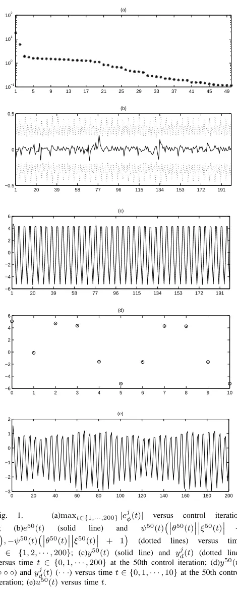
respectively. In order to verify the robustness against varying initial resetting error ej_{(0) and the non-repeatable random} disturbance dj_{(t), we show max}

t∈{1,···,200}|ejφ(t)| with re-spective to iteration j in Fig. 1(a). The asymptotical con-vergence proves the technical result given in (t2) of main theorem. Since the learning process is almost completed at the 50th iteration, the learning errore50(t)is shown in Fig. 1(b). It clearly proves (t3) of the main theorem since the trajectory ofe50(t)satisfies−ψ50(t)¡¯¯θ50(t)¯¯¯¯ξ50(t)¯¯+1¢≤

e50_{(t) ≤ψ}50_(t)¡¯_¯θ50_(t)¯_¯¯_¯ξ50_(t)¯_{¯+ 1}¢_{, t ∈ {1,· · ·,200} in}

Fig. 1(b). Since the nice output tracking performance at the 50th iteration are achieved, we show the relation between system outputy50_{(t)and desired trajectoryy}50

d (t)in Fig. 1(c) for t ∈ {0,1,2,· · ·,200}. To see the control behavior that

y50_{(t)is close toy}50

d (t)fort∈ {0,1,2,· · ·,200}except the initial oney50_{(0), the trajectories betweeny}50_(t)andy50

d (t) are shown again in Fig. 1(d) but only for the time sequence

t ∈ {0,1,2,· · ·,10}. It is clear that y50_{(t) converges to}

y50

d (t) after t ≥ 1. Finally, Fig. 1(e) shows the bounded learned control force u50(t).

1 5 9 13 17 21 25 29 33 37 41 45 49

10−1 100 101 102

(a)

1 20 39 58 77 96 115 134 153 172 191

−0.5 0 0.5

(b)

1 20 39 58 77 96 115 134 153 172 191

−6 −4 −2 0 2 4 6

(c)

0 1 2 3 4 5 6 7 8 9 10

−6 −4 −2 0 2 4 6

(d)

0 20 40 60 80 100 120 140 160 180 200

−3 −2 −1 0 1 2

(e)

Fig. 1. (a)maxt∈{1,···,200}|ejφ(t)| versus control iteration

j; (b)e50_{(t) (solid line) and ψ}50_(t)¡¯¯_θ50_(t)¯¯¯¯_ξ50_(t)¯¯ ₊ 1¢,−ψ50_(t)¡¯¯_θ50_(t)¯¯¯¯_ξ50_(t)¯¯ _{+ 1}¢ _{(dotted lines) versus time} t ∈ {1,2,· · ·,200}; (c)y50_{(t) (solid line) and y}j

d(t) (dotted line) versus timet ∈ {0,1,· · ·,200} at the 50th control iteration; (d)y50_(t)

(◦ ◦ ◦) andyj_d(t)(· · ·) versus timet∈ {0,1,· · ·,10}at the 50th control iteration; (e)u50_{(t)versus timet.}

VI. CONCLUSION

[image:5.595.309.544.48.633.2]

that the control direction can be unknown and the input disturbance can be non-repeatable. Three control parameters in this RAILC are applied to compensate for the uncertainties from the unknown system parameters and input disturbance. By using a Lyapunov like analysis, it is shown that the control parameters and internal signals are bounded along the time axis for all iterations and the tracking error will asymptotically converge to a tunable residual set which is bounded by the width of boundary layer.

ACKNOWLEDGMENT

This work is supported by Ministry of Science and Tech-nology, Taiwan, under Grants MOST103-2221-E-211-010 and MOST 103-2221-E-211-012.

REFERENCES

[1] K. L. Moore, J. X. Xu, “Special issue on iterative learning control,”

Int. J. Contr., Vol. 73, ,pp. 819-823, 2000.

[2] D. A. Bristow, M. Tharayil, A.G. Allyne, “A survey of iterative learning,” IEEE Control Systems Magazine, Vol. 26, pp. 96-114, 2006. [3] H. S. Ahn, Y. Chen, and K. L. Moore, “Iterative learning control: Brief survey and categorization,” IEEE Transactions on Systems Man

and Cybernetics, Part C - Applications and Reviews, Vol. 37, No. 6,

pp. 1099-1121, Nov 2007.

[4] C. J. Chien and C. Y. Yao, “Iterative learning of model reference adaptive controller for uncertain nonlinear systems with only output measurement,” Automatica, Vol. 40, No. 5, pp. 855-864, 2004. [5] A. Tayebi and C.J. Chien, “A unified adaptive iterative learning control

framework for uncertain nonlinear systems,” IEEE Transactions on

Automatic Control, Vol. 52, No. 10, pp. 1907-1913, 2007.

[6] I. Rotariu, M. Steinbuch and R. Ellenbroek, “Adaptive iterative learning control for high precision motion systems,” IEEE Transactions on

Control Systems Technology, Vol. 16, No. 5, pp. 1075-1082, 2008.

[7] W. S. Chen, J. Li and J. Li, “Practical adaptive iterative learning control framework based on robust adaptive approach,” Asian Journal

of Control, Vol. 13, No. 1, pp. 85-93, 2011.

[8] T. Ngo, Y. Wang, T.L. Mai, J. Ge, M.H. Nguyen and S.N. Wei, “An adaptive iterative learning control for robot manipulator in task space,”

International Journal of Computers, Communications and Control ,

Vol. 7, No. 3, pp. 510-521, 2012.

[9] R. H. Chi, Z. S. Hou and S. L. Shu, “Discrete-time adaptive iterative learning from different tracking tasks with variable initial conditions,”

Proceedings of the 26th Chinese Control Conference, pp. 791-795,

2007.

[10] R. H. Chi, Z. S. Hou and J. X. Xu, “Adaptive ILC for a class of discrete-time systems with iteration-varying trajectory and random initial condition,” Automatica, Vol. 44, pp. 2207-2213, 2008. [11] R. H. Chi, S. S. Lin and Z. S. Hou, “A new discrete-time adaptive

ILC for nonlinear systems with time-varying parametric uncertainties,”

Acta Automatica Sinica, Vol. 34, Issue 7, pp. 805-808, 2008.

[12] X. D. Li, T. F. Xiao and H. X. Zheng, “Adaptive discrete-time iterative learning control for non-linear multiple input multiple output systems with iteration-varying initial error and reference trajectory,” IET Control

Theory and Applications, vol. 5, issue 9, pp. 1131-1139, 2010.

[13] C.J. Chien and Y.C. Wang, “Adaptive iterative learning control for a class of nonlinear discrete-Time systems with random bounded dis-turbance,” 2012 International Automatic Control Conference, Taiwan, 2012.

[14] H. Chen and P. Jiang, “Adaptive iterative learning control for nonlinear systems with unknown control gain,” Journal of Dynamic Systems,

Measurement, and Control, Vol. 126, no. 4, pp. 916 920, 2004. [15] J.X. Xu and R. Yan, “Iterative learning control design without a priori

knowledge of the control direction,” Automatica, Vol. 40, no. 10, pp. 1803 1809, 2004.

[16] P. Jiang and Y. Q. Cheng, “Adaptive iterative learning control for a class of nonlinear systems with unknown control directions,” The Open

Automation and Control System Journal, Vol. 1, no. 4, pp. 20-26, 2008.

[17] Miao Yu, Jianliang Zhang and Donglian Qi, “Discrete-time adaptive iterative learning control with unknown control directions,”

Interna-tional Journal of Control, Automation and Systems, Vol. 10, Issue 6,

pp 1111-1118, 2012.

[18] Miao Yu, Jiasen Wang and Donglian Qi, “Discrete-time adaptive iter-ative learning control for high-order nonlinear systems with unknown control directions,” International Journal of Control, Vol. 86, Issue 2, 2013.

[19] Weili Yan and Mingxuan Sun, “Adaptive iterative learning control of discrete-time varying systems with unknown control direction,”

International Journal of Adaptive Control and Signal Processing, Vol.