Multi-vendor and Multi-buyer Collaborative
Planning Forecasting and Replenishment Model
C.M. Su, K.Y. Chang, Y.T Chou and Y.S. Pan, Member, IAENG
Abstract—This article proposes a two-echelon integrated production-inventory supply chain model. We assume that the production process is unreliable. The defective items will be send back to the upstream (vendors) and the buyers will receive the repaired products after the reworking. In order to forecast buyer’s demand more precisely, we design a linear regression equation, which based on past years demand. The objective is to minimize the joint total cost, and present the proposed model and optimal solution by numerical examples.
Index Terms—supply chain; inventory; integer-multiplier policies; defective items;
I.
I
NTRODUCTIONn today’s competitive market, an enterprise has to be able to develop sustainably and stay competitive, finding partner and alliance has become a trend nowadays, forming a vertical supply chain which integrates from up to down in order to optimize the profit of the whole supply chain (or minimize the cost). After forming the relationship, the strategy of management is vital, one of the sectors is the strategy of inventory management. Since the cost of the inventory accounts for a high proportion of supply chain, many experts has been making research on inventory management for many years. Harris [1] was the first researcher who developed economic order quantity (EOQ) model, this model was consisted by a single company’s ordering costs and holding costs. In the viewpoint of the supply chain management (SCM), collaborating closely with the members of supply chain is certainly necessary, so Harris’ research didn’t meet the actual situation. In order to meet the SCM’s status, Goyal [2] was the first researcher to develop a single-vendor single-buyer’s integrated inventory model. Banerjee[3] proposed Joint Economic Lot Size (JELS), assumedorder quantity will not be shipped in batch, but will be shipped to the buyer after production run. Goyal [4]
Manuscript received September 14, 2015.
Chien-Min Su is with Department of Transportation Science, National Taiwan Ocean University, No.2, Beining Rd., Jhongjheng District, Keelung City 202, Taiwan, R.O.C. (phone: +886-2-24622192#7037; fax:+886-2-24633745; e-mail: [email protected])
Ki-Yin Chang is with Department of Merchant marine, National Taiwan Ocean University, No.2, Beining Rd., Jhongjheng District, Keelung City 202, Taiwan, R.O.C. (phone: +886-2-24622192#3019; e-mail:
Yen-Ting Chao is with Department of Information Management, Taipei Chengshih University of Science and Technology, No. 2, Xueyuan Rd., Beitou, 112 Taipei, Taiwan, R.O.C. (e-mail: [email protected])
Yu-Sheng Pan is with Department of Transportation Science, National Taiwan Ocean University, No.2, Beining Rd., Jhongjheng District, Keelung City 202, Taiwan, R.O.C. (e-mail:[email protected])
extended Banerjee’s [3]research, discussion lot size per production is an integer multiple of the buyer’s optimal order quantity. Lu [5] developed single-vendor multi-buyer’s integrated inventory model, and assumed each shipping size were equal. Goyal [6] modified Lu’s [5] point of view, proved that different delivery policies can get better results. Hill [7] extended Goyal [6] and Lu’s [5] model, proposed the lot size of each shipment will between 1 ~ P/ D multiplier during production run. Ha and Kim [8] assumed lot size per production run and buyer’s order quantity are equal, and deliver to buyer divided into N times. Goyal and Nebebe [9] extended Goyal [6] and Hill’s [7] research, proposed a new model and got a better optimal order quantity. Pan and Yang [10] developed a model which concerned controllable lead time and the size of each shipment are equal. Kelle et al. [11] proposed a model which the lot size per production run is m times greater than shipment size, m is an integer multiplier. The vendor will divided the shipment size into n times and deliver to buyer, n is not necessarily equal to m. Pan and Yang [12] who developed an integrated inventory model which used fuzzy theory, assumed the demand rate and production rate were not a fixed value, and then derived the optimum order quantity. Yang and Lo [13] discussed a single-vendor multi-buyer’s system, and lead time is variable. Subrata Mitra [14] proposed two-echelon close-loop supply chain, and discussed variation with traditional supply chain. J.K. Jha [15] added service level constraints in integrated inventory model, and considered the lead time was not fixed.
Our purpose in this article is to minimize the expected joint total cost. We will develop multi-vendor multi-buyer inventory model with defective rate. We set that the lot produced at each stage is delivered in equal shipments to the downstream (buyers), and shipments are delivered as soon as they are produced, not to wait until a whole lot is produced.
We first defined the parameters and assumptions in Section II, and then we started to develop the integrated inventory model in Section III. In Section IV, we solved the model to get the optimal solution and showed numerical examples in Section V. In the end, we summarized the conclusions in Section VI.
II.
N
OTATIONS ANDA
SSUMPTIONSTo develop a two-echelon integrated inventory model, the notations and assumptions are used in developing the model are as follow.
A. Notations
,
,
The basic cycle time of a buyer.
Integer multiplier for the cycle time at vendor's stage. Demand rate for vendor
rodu
.
P ction rate for
v
v g
v g
T K
D g
P
aterials unit stocking-holding cost per unit per year for vendo
vendor .
r.
Finished product unit stocking-holdi Number of vendors.
ng c M
v v
s
g
h n h
,
ost per unit per year for vendor.
Set up cost per production run for vendor. Manufacturing cost per unit for vendor. Demand rat
v
r
b j
S Q
D , , , ,
ˆ
ˆ ˆ
e for buyer .
Finished product unit stocking-holding cost per unit
Number of buyer per year for buyer.
s.
b j b j b j b j n
b b
b
D E Q
j
h
S n
Ordering cost for vendor. Recycling cost for vendor. Repairing cos
Unit screening cost for buyer t for vendor.
. R
L d X
Unit purchasing cost
Screening rate for buyer. for buyer. rate (1- ) for
Discount , 5
buyer. ercentag f
P e o
B
m k
mkY
,
,
P
ˆ
Slope of population
defective products can not be repaired. ercentage of defec
regression function. ˆ
Intercept of
tive products.
b j
b j
Y
,
,
,
( , )
population regression function. ˆ
Forecasted demand. Total cost for vendor . Total cost for buyer . Joint total cost of
v b j
v g
b j
k T
E
TC g
TC j
JTC whole supply chain.
B. Assumptions
(i) This paper is based on multi-vendor and multi-buyer for single item.
(ii) The production rate is finite. (iii) Shortages are not allowed
(iv) Because of shortages are not allowed, non-defective product’s production rate must higher than buyer’s demand.
(v) Quantity discount and defective rate has direct relation.
(vi) Returned defective production will be repaired, but not fully repaired.
(vii) Demands are equal at all echelons. Based onpulling
production
1 , 1 ,
n n
j g
b v
b j v g
D D
(viii) Each stage of the supply chain’s cycle time are equal and the cycle time at each stage is an integer multiplier of the cycle time at the adjacent downstream stage. The cycle time of vendor is
*
v v
T K T
III.
M
ODELF
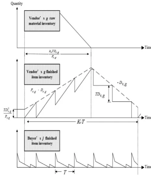
ORMULATIONIn this section, we joint vendor and buyer’s total cost into integrated inventory model. In the Fig. I, the start of a cycle the inventory level equal to 2
, / , . v g v g
TD P Then the inventory
level starts increasing at the ratePv g, Dv g, until it reaches its
maximum level
Pv g, Dv g,
k TDv v g, /Pv g, .Then it is consumedat the rateDv g, until the end of the cycle. The vendor of the
[image:2.595.56.552.304.753.2] [image:2.595.301.546.464.751.2]A. The vendor’ s annual total cost
In each production run, the vender’s cost includes set up cost, manufacturing cost, holding cost, recycling cost, repairing cost. The vendor’s total annual cost consists of the following elements.
(i) Set up cost v
v
S K T
(ii) Manufacturing costQ Pr v j, (iii) Recycling costRKYPv g,
(iv) Repairing costLYDv g,
(v) Holding cost
2 2
, ,
,
, ,
2 ( 1)
2 2
s v g v v g
v v v g
v g v g
h TD h T D
k k D
P P
B. The buyer’s annual total cost
In each production run, the vender’s cost includes ordering cost, screening cost, purchasing cost, holding cost. The buyer’s total annual cost consists of the following elements.
(i) Set up cost Sb
T
(ii) Screening cost
, 1 b j dD kY(iii) Purchasing cost
D
b j,
1
(iv) Holding cost is given by:
2 2 2 , , , 2 2 2 2 , , 1 1 2 12 1 2 1
1
2 1 1 1
b b j b j b j
b b j b j
D T Y D k YT
D T Y h
T X kY kY kY
Y kY
h D T D Y
Y
kY X kY kY
[image:3.595.320.546.320.587.2]
Fig. II. The buyer’s inventory level
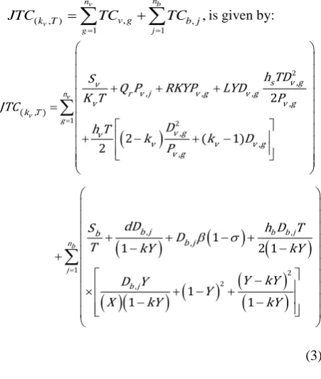
C. The joint annual total cost
(i) The vendor’s annual cost is given by:
2 2 , , , , , , , , 22 ( 1)
2
s v g v
v r v g v g v g
v v g
v g v
v v v g
v g
h TD
S
TC
Q P
RKYP
LYD
K T
P
D
h T
k
k
D
P
(1) (ii) The buyer’s annual cost is given by:
2 2 , , , , 11 2 1
1
1 1
b j b b j
b
b b j
b j
dD h D T
S
TC D
T kY kY
D Y Y kY
Y
X kY kY
(2)
(iii)The joint annual total cost for the whole supply chain
1 1
,
( , ) , ,
v
bv
n n
g j
v g
k T b j
JTC TC TC is given by:
2 1 2 , , , , , ( , ) , , , 22 ( 1)
2 v v n g
s v g v
r v j v g v g
v v g
k T
v g v
v v v g
v g
h TD S
Q P RKYP LYD
K T P
JTC
D h T
k k D
P
1 2 2 , , , , 11 2 1
1 1 1 b n j
b b j
b j
b j b
b j
dD h D T
S
D
T kY kY
Y kY D Y
Y
X kY kY
(3)IV.
S
OLUTIONP
ROCEDUREFor givenKv , clearly ( , ) v k T
JTC is convex function in
T
for
T
> 0.Therefore, minimum cost at a unique value ofT
.To determine the minimum cost, we taking the derivative of ( , )v k T
JTC with respect to
T
, letJTC k T( , )/v T 0, which yields
1
2
2 1
v b
v b v
v b
S
n
S
K Y
k
T
n
K
h
Yk
where
2 2
2
1
1
, ,
, , ,
, ,
1
= 1
1 1
2
1 2
n
j
n
g b
v
b j b j
v g v g v v g s
v v
v g v g
Y k D Y
D Y
Yk Yk X
D D K D h
h K
P P
Because to forecast buyer’s annual demand, theDb j, will be
substituted byEˆb j, , and
1
2 1
, , ,
,
, ,
, ,
, ˆ
ˆ ˆ 5
ˆ 1 ~ (6)
ˆ
ˆ 1 ~
b j b j b j n
t b j n
t
b j b j
n
t j j t j j
b
t j j
b j
E Q
Q Q F F
n j
Q Q
n
F j (7)
Algorithm
In order to obtain the minimum values of ( , ) v k T
JTC , we
following these steps:
Step 1. DetermineDb j, by Eq.(5).
Step 2. Calculate the valueT kv of using Eq.(4). Step 3. Compute ( , kv)
v
JTC k T using Eq.(3).
Step 4. Let
k
v =k
v1 , repeat steps 1 to 3 to find
( , kv ) v
JTC k T .
Step 5. If 1
( , kv) ( 1 , kv ),
v v
JTC k T JTC k T returned to Step 4. Otherwise, the optimal solution
is
1
, 1,
kv
v v
k T k T
V.
N
UMERICALE
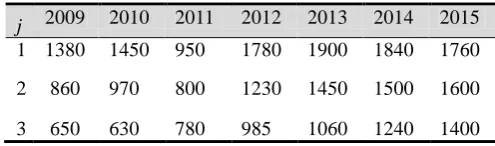
XAMPLEThe proposed analytic solution procedure is applied to solve the following numerical example. We set number of vendor and buyer is 3, hs$0.9/units, hv$2/units, Sv$400/cycle, Sb
$10/units, $3/units, $6/units, $0.5/units, 6000 units/year, $9/unit
$150 /cycle, = 0.7, 0.03,
0.9 37, and buyer's demand in past 7 years is shown in Table I
s, . 1
r
Q R L
d X B m
k Y
kY
[image:4.595.47.287.54.137.2]
Table I.
The data of buyer’s demand(units/year)in past 7 years.
Before forecasting buyer’s demand, we calculate Eq.(5),
and get the value
, , ,
ˆ ˆ
b j
b j by using Eq.(6) and Eq.(7).Therefore, we obtain Db,11727units/year ,unit 1649 s/ arye
D , D 1588units/y a ,e r D and
,
v g
P is shown in Table II.
Table II.
The data of vendor’sDv g, andPv g, .
Applying the algorithm, we obtain the optimal solution as
follows: buyer’s cycle time isT0.273(year),kv6,the vendor’s cycle time isTv 1.636(year), and the joint total
cost is $201,204.14.
We do sensitivity analysis to observe the JTC*under
different values of T, y and k, the results were shown in Table III and Table. IV.
Table. III.
Sensitivity analysis for Y and k.
Table. IV.
Sensitivity analysis for replenishment cycle T.
VI.
C
ONCLUSIONIn this paper, we develop two-echelon integrated inventory model with unreliable process. Defective rate and repaired rate are important factors to affect the inventory policy. The goal of this paper is to optimize the joint total cost of the supply chain network with coordinating decision-making.
From Table. III, we can know the joint total cost will grow with increased k and Y, so defective products cause additional time and cost on purchasing and production. In this model, production patterns is pulling production, so back end demand of supply chain is the most important. Base on collaborative planning, forecasting and replenishment
(CPFR), we design a linear regression to forecast buyer’s
demand. According to forecast result, the decision-makers or managers can do a right decision to avoid enterprise operating loss.
Through Table. IV, we can know the joint total cost will increase along with longer replenishment cycle time, representing its affect the overall cost significantly. As mentioned above, we derive buyer’s replenishment cycle time (T) from this model, which is the optimum value to whole supply chain, and vendor can predict manufacturing cycle time by multiply an integer number(kv), thus enhance
j 2009 2010 2011 2012 2013 2014 2015 1 1380 1450 950 1780 1900 1840 1760
2 860 970 800 1230 1450 1500 1600
3 650 630 780 985 1060 1240 1400
g Dv g, (units/year) Pv g, (units/y r)ea
1 1550 5500
2 1640 4500
3 1774 3000
JTC* Y k
-25% +25% -25% +25%
JTC $201,204 $200,77
7
$201,63 0
$200,97 5
$201,43 3
Compare with JTC*
-$426 +$426 -$228 +$229
JTC* T
-25% +25%
JTC $201,204.14 $199,807.74 $209,918
Compare with JTC*
[image:4.595.44.292.639.712.2]Finally, we will improve our further research in more real-world complexities, such as add more factors into linear regression function to make forecasting result more accurate, and cooperate real case to get the actual data that can illustrate real numerical examples to our future research.
REFERENCE
[1] F. W. Harris, “How Many Parts to Make at Once”, Operations Research, Vol. 38, No. 6, pp. 947-950, 1913.
[2] S.K. Goyal, “An Integrated Inventory Model for a Single Supplier single Customer Problem,” International Journal of Production Research, Vol. 15, No. 1, pp.107-111, 1976.
[3] A. Banerjee, “A joint economic-lot-size model for purchaser and vendor”, Decision Sciences, Vol. 17, pp. 292-311, 1986.
[4] S.K. Goyal, “A Joint Economic-lot-size Model for Purchaser and Vendor: A Comment”, Decision Sciences, Vol. 19, No. 1, pp. 236-241, 1988.
[5] L. Lu, “A one-vendor multi-buyer integrated inventory model”, European Journal of Operational Research.Vol.81, No 2, pp 312-23. 1995.
[6] S.K. Goyal, “one-vendor multi-buyer integrated inventory model: A comment”, European Journal of Operational Research, Vol 82, No 1, pp 209-210, 1995.
[7] R.M Hill, “The Single-vendor Single-buyer Integrated Production-inventory Model with a Generalized Policy”, European Journal of Operational Research, Vol. 97, No 3, pp. 493-499. 1997
[8] D. Ha, & S.L. Kim, “Implementation of JIT Purchasing: An Integrated Approach”, Production Planning and Control, Vol. 8, No. 2, pp. 152-157. 1997.
[9] S.K. Goyal, & F. Nebebe, “Determination of Economic Production-shipment Policy for a Single-vendor–single-buyer System”, European Journal of Operational Research, Vol.121, pp.175-178, 2000.
[10] C.-H. J. Pan, & J. S. Yang, “A study of an integrated inventory with controllable lead time,” International Journal of Production Research, Vol. 40, No. 5, pp.1263-1273. 2002.
[11] P. Kelle, & F. Al-khateeb, & P.A. Miller, “Partnership and negotiation support by joint optimal ordering/setup policies for JIT”, International Journal of Production Economics, Vol. 81-82, pp.431-441. 2003
[12] C.H. Pan, and M.F. Yang, “Integrated inventory models with fuzzy annual demand and fuzzy production rate in a supply chain”, International Journal of Production Research, Vol.46, No. 3, pp.753-770. 2008.
[13] M.F. Yang and M.C. Lo, “Considering single-vendor and multiple-buyers integrated supply chain inventory model with lead time reduction”, Proceedings of the Institution of Mechanical Engineers, Part B, Journal of Engineering Manufacture, Vol.225, pp.747-759. 2011.
[14] S. Mitra, “Inventory management in a two-echelon closed-loop supply chain with correlated demands and returns”, Computers & Industrial Engineering, Vol.62, No. 4. pp, 870-879. 2012.
[15] J.K. Jha, and K. Shanker, “Single-vendor multi-buyer integrated production-inventory model with controllable lead time and service level constraints”, Applied Mathematical Modelling, Vol. 37,No. 4, pp. 1753-1767, 2013.
[16] P.M. Ghare, and G.H. Schrader, “A model for exponential decaying inventory”, Journal of Industrial Engineering, Vol.14, pp. 238-243, 1963.
[17] R.P. Covert, G.C. Philip, “An EOQ Model for Items with Weibull Distributed Deterioration”, AIIE Trans. Vol. 5, No. 4, pp. 323-326, 1973.
[18] J.M. Chen, “An inventory model for deteriorating items with time-proportional demand and shortages under inflation and time discounting ”, International Journal of Production Economics, Vol.55, No.1, pp. 21-30, 1998.
[19] H.M. Wee, and S.T. Law, “Replenishment and pricing policy for deteriorating items taking into account the time-value of money”, International Journal of Production Economics, Vol 71, No, 1–3, pp, 213–220,2001.
[20] M.F. Yang and Y. Lin, “Applying the Linear Particle Swarm Optimization to a Serial Multi-echelon Inventory Model”, Expert Systems With Applications, Vol.37, No. 3, pp. 2599-2608,2010.