Fast Sequential Parameter
Inference for Dynamic State Space
Models
A thesis submitted to University of Dublin, Trinity College in partial fulfilment of the requirements for the degree of
Doctor of Philosophy
Department of Statistics, School of Computer Science and Statistics, University of Dublin, Trinity College
February 2012
This thesis has not been submitted as an exercise for a degree at any other University. Except where otherwise stated, the work described herein has been carried out by the author alone. This thesis may be borrowed or copied upon request with the permission of the Librarian, University of Dublin, Trinity College. The copyright belongs jointly to the University of Dublin and Arnab Bhattacharya.
Arnab Bhattacharya
Abstract
Many problems in science require estimation and inference on systems that generate data over time. Such systems, quite common in statistical signal processing, time series analysis and econometrics, can be stated in a state-space form. Estimation is made on the state of the state-space model, using a sequence of noisy measurements made on the system. This difficult problem of estimating the parameters in real time, has generated a lot of interest in the statistical community, especially since the latter half of the last century.
One area that is particularly important is the estimation of parameters which do not evolve over time. The parameters in the dynamic state-space model generally have a non-Gaussian posterior distribution and holds a nonlinear relationship with the data. Sequen-tial inference of these static parameters requires novel statistical techniques. Addressing the challenges of such a problem provides the focus for the research contributions pre-sented in this thesis. A functional approximation update of the posterior distribution of the parameters is developed. The approximate posterior is explored at a sufficient number of points on a grid which is computed at good evaluation points. The grid is re-assessed at each time point for addition/reduction of grid points. Bayes Law and the structure of the state-space model are used to sequentially update the posterior density of the model parameters as new observations arrive. These approximations rely on already existing state estimation techniques such as the Kalman filter and its nonlinear extensions, as well as integrated nested Laplace approximation. However, the method is quite general and can be used for any existing state estimation algorithm.
Acknowledgements
Firstly I would like to express my thanks and gratitude to my supervisor Professor Simon Wilson. After spending a few years away from academia, I was extremely slow to start with. Simon has always been extremely patient in dealing with me and my questions and has always been there when I needed direction. He has been an excellent supervisor, always encouraging me with the topics that interest me and also giving me space to make my own observations. His knowledge of statistics is astounding and his continuing enthusiasm for my work has never ceased to amaze me. He introduced me to the world of Bayesian statistics and I greatly appreciate the opportunities he provided for me in these years. I thank my stars that I have someone as supervisor, who would allow the bad routine of work I follow. I sincerely hope that our collaboration will continue into the future.
Next a big thanks to three people in our department, Brett Houlding, Louis Aslett and Ji Won Yoon. The beginning of our work has been possible due to the assistance I got from Brett and his vision and clarity on the subject as a whole. Louis has been an excellent friend and partner for discussing anything related to statistics that would come to my mind. Also a big thank you for introducing me to the world of efficient and intelligent programming. And finally, it is due to Ji Won that my knowledge in the specific area of my topic increased many fold. He always had an answer to any question I had in mind. Another big thank you to Susanne, Tiep, James, Jason, Thinh and everybody else in our office, room 108.
I would like to thank my parents and my brother who have always been encouraging and supportive of my studies. It is because of their support that I could leave what I was not enjoying and take up what interests me. A thank you must go to the great group of friends, both here and in Kolkata who had always been there no matter what. Thank you Deb, Aurab, Ani and Vee for been there, high or low.
Contents
Decleration v
Summary v
Acknowledgements v
1 Introduction 1
1.1 Motivation . . . 1
1.1.1 Motivation for Statistical Research . . . 3
1.2 Research Contributions . . . 4
1.3 Overview of Chapters . . . 5
2 Time Series and Sequential Estimation 7 2.1 Time Series and Forecasting . . . 7
2.2 Time Series Models . . . 9
2.2.1 Classical Time Series . . . 9
2.2.2 Inference and Prediction for ARIMA . . . 10
2.3 State space models . . . 11
2.3.1 Dynamic Models . . . 14
2.3.2 Dynamic Linear Models . . . 15
2.3.3 Nonlinear/Non-Gaussian Models . . . 16
2.4 Inference for State Space models . . . 16
2.4.1 Kalman Filter . . . 18
2.4.2 Extensions of the Kalman Filter . . . 19
2.4.2.1 Extended Kalman Filter . . . 20
2.4.2.3 Other Filters . . . 23
2.4.2.4 Divergence . . . 24
2.4.3 Sequential Monte Carlo Methods . . . 24
2.4.3.1 Sequential Importance Sampling Filter (SIS) . . . 25
2.4.4 Grid Based Filters . . . 30
2.5 Off-line methods . . . 32
2.5.1 Expectation Maximization . . . 32
2.5.2 Variational Bayes . . . 32
2.5.3 Expectation Propagation . . . 33
2.6 Parameter Estimation in State-Space Models . . . 34
2.6.1 Kalman filter based methods: . . . 35
2.6.2 Sequential Monte Carlo based methods: . . . 36
2.7 Conclusion . . . 38
3 Statistical Methodology 39 3.1 Statistical Inference . . . 39
3.1.1 Interpretation of Probability . . . 40
3.1.2 Prior Distribution . . . 41
3.1.3 Likelihood Function . . . 41
3.1.4 Posterior Distribution . . . 42
3.1.5 Prior Elicitation . . . 43
3.1.6 Predictive Distribution . . . 45
3.2 Numerical Problems in Bayesian Inference . . . 45
3.3 Markov Chain Monte Carlo . . . 47
3.3.1 Markov Chains and Detailed Balance . . . 47
3.3.2 The Metropolis-Hastings Algorithm . . . 49
3.4 Integrated Nested Laplace Approximation (INLA) . . . 50
3.4.1 Gaussian Markov Random Field (GMRF) . . . 50
3.4.2 Gaussian Approximation . . . 51
3.4.3 INLA . . . 52
3.5 Kalman Filter . . . 54
4 Sequential Parameter Estimation in State Space Models 58
4.1 Introduction . . . 58
4.2 Initial Steps with INLA . . . 60
4.3 Sequential Bayesian Estimation ofθ . . . 61
4.3.1 Crude Solution . . . 63
4.3.2 Computation of P(Xt|Y1:t−1, θ) and P(Xt|Y1:t, θ) for Equation (4.3.4) . . . 64
4.4 Algorithm . . . 65
4.5 Updating the Grid . . . 65
4.5.1 Motivation . . . 65
4.5.2 New Internal Grid point . . . 68
4.5.2.1 Identifying when and where to add a new internal point . . 68
4.5.2.2 Calculating the posterior and other necessary values at new grid point(s) . . . 69
4.5.2.3 The Generalized Additive Model . . . 72
4.5.2.4 Multivariate Adaptive Regression Splines . . . 73
4.5.2.5 Problem with Smoothing methods . . . 75
4.5.2.6 Interpolation . . . 76
4.5.3 New External Grid point . . . 79
4.5.3.1 Method I . . . 83
4.5.3.2 Method II . . . 85
4.5.4 Combination of adding points internally and externally . . . 88
4.5.5 Computing other statistics at the new grid points . . . 89
4.6 Final Algorithm for Updating the Posterior Density of θ|Y1:t . . . 90
4.7 Conclusion . . . 91
5 Correction to Improve Posterior Density of the Parameters 92 5.1 Problem encountered in the current method . . . 92
5.1.1 Explanation of problem . . . 92
5.1.2 Cause of the problem . . . 94
5.2 Solution to this problem/Dealing with outliers . . . 96
5.2.2 Application of Cseke and Heske’s method in our algorithm . . . 98
5.3 Implementation . . . 99
5.4 Conclusion . . . 101
6 Application of Sequential Algorithm to Simulated Examples 102 6.1 Goal of the Application . . . 102
6.2 Performance Measures . . . 103
6.2.1 Mode and Probability intervals . . . 103
6.2.1.1 Estimation of Mode . . . 104
6.2.1.2 Estimation of 95% marginal probability limits . . . 104
6.2.2 Mahalanobis Distance . . . 107
6.2.3 Coverage Proportion . . . 108
6.2.4 Computation Time . . . 108
6.3 Application of different algorithms in different models . . . 109
6.4 Linear Model with Additive Gaussian Errors . . . 109
6.4.1 Method 1: Crude Method of Chapter 4 . . . 111
6.4.1.1 Computation of P(Xt|Yt, θ) . . . 111
6.4.1.2 Application of the Crude Method . . . 111
6.4.2 Method 2: Sequential Update of P(θ|Y1:t) . . . 113
6.4.2.1 Computation ofP(Xt|Y1:t−1, θ) andP(Xt|Y1:t, θ) for Se-quential Update . . . 113
6.4.2.2 Results after implementing the algorithm . . . 115
6.4.3 Particle filter . . . 119
6.4.4 Comparison of the two methods . . . 121
6.5 Nonlinear Model . . . 126
6.5.1 Method Used: Sequential Update . . . 126
6.5.1.1 Computation ofP(Xt|Y1:t−1, θ) andP(Xt|Y1:t, θ) for Se-quential Update . . . 126
6.5.1.2 Performance of the Sequential Algorithm . . . 130
6.5.2 Particle filter . . . 132
6.5.3 Comparison of the two methods . . . 132
6.6.1 Method Used: Sequential Update . . . 136
6.6.1.1 Computation ofP(Xt|Y1:t−1, θ) andP(Xt|Y1:t, θ) for Se-quential Update . . . 137
6.6.1.2 Performance of the Sequential Algorithm . . . 138
6.6.2 Particle filter . . . 138
6.6.3 Comparison of the two methods . . . 141
6.7 Conclusion . . . 144
7 Conclusion and Further Work 147 7.1 Conclusion . . . 147
7.2 Future Work . . . 149
7.2.1 Restriction on the number of static parameters . . . 149
7.2.2 Convergence of the filter . . . 150
7.2.3 Computation of log-posterior and necessary statistics at new grid points . . . 151
7.2.4 Application on real life problem . . . 151
7.3 Final Comments . . . 151
A Linear models 153 A.1 Example 1 . . . 153
A.2 Example 2 . . . 153
A.3 Example 3 . . . 156
A.4 Example 4 . . . 156
B Nonlinear models 159 B.1 Example 1 . . . 159
B.2 Example 2 . . . 159
C Non-Gaussian models 162 C.1 Example 1 . . . 162
C.2 Example 2 . . . 164
C.3 Example 3 . . . 164
List of Figures
2.1 DAG representing the general state space model where the parameters are not shown. . . 12 2.2 Fit of filtered levelxt over data recorded from Three Rock antenna, south
of Dublin. The fit is done using a state space model with three unknown parameters. . . 13
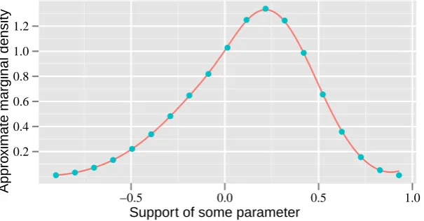
4.1 This plot shows the posterior marginal density of a parameter from some toy example. The posterior density denoted by the points on the plot clearly shows that grid points on the tail have negligible posterior marginal values, which can be dropped to facilitate computation. Also a refinement of grid is required, since the supporting grid is shrinking and new points are required to be added internally. . . 67 4.2 The posterior marginal density in this plot clearly shows that new points
need to be added to the left of the existing grid. Also some existing grid points from the right tail can be dropped since the value of the marginal density at those points are very small. . . 68 4.3 Single point added between two points for a single variable. . . 69 4.4 The×’s and thein this plot shows possible combinations of new internal
points for each of the two parameters. The points (θ1×, θ21),(θ×1, θ22),(θ11, θ2×) and (θ2
1, θ
×
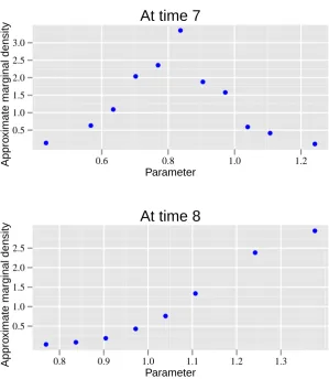
2) require interpolation on a single variable. Bivariate rule is needed for the combination (θ×1, θ×2). . . 69 4.5 This plot has blue circles denoting the posterior marginal density and black
circles denote the grid points representing the support of the density. The red circles are new points which need to be added to the existing grid and are added using the rule explained in Section 4.5.2.1. . . 70 4.6 This plot shows the approximate posterior marginal density at the new
4.7 This plot also shows the approximate posterior marginal density of the new internal points in the original grid as in Figure 4.5. The red circles denoting the approximate posterior at internal points are computed using GAM. Note the over fit in the density for the new points. . . 73 4.8 This plot shows the approximate posterior marginal density of the new
internal points calculated using MARS. Note that the smoothing is better for this methodology than GAM, for the toy example that we have used in Figure 4.5. . . 75 4.9 This plot is exactly same as Figure 4.4. This is provided here once more
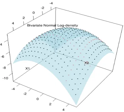
to better explain the bivariate interpolation rule of calculating the log-posterior density. . . 77 4.10 Surface plot of bivariate normal log-density. The black points visible on
the blue surface reflect the log-density values of the existing grid and the red points reflect the interpolated log-density values at the newly added internal points. . . 80 4.11 In this plot we have compared the performance of linear interpolation
tech-nique in computation of the log-density value of a new added internal point. The computed approximate log-density value at this point is compared with the true conditional log-density of X2|X1 =x1. Note that there is only a very small difference between the values. . . 80 4.12 Single point added outside the support of the grid for a single variable. . . . 81 4.13 This plot shows all possible combinations of new external points for each
of the two parameters θ×1 and θ×2 respectively. The four points for which log-posterior density is calculated using linear interpolation are (θ1×, θ21), (θ1×, θ22), (θ11, θ×2) and (θ12, θ×2). Bivariate interpolation is used on the single point (θ×1, θ×2). . . 81 4.14 This plot is same as Figure 4.2 and is shown here for the sake of convenience
in understanding Section 4.5.3. . . 82 4.15 This plot shows what we are talking about in Section 4.5.3.1. The line
4.16 This plot represents a situation using a toy example where the true support of a parameter “moves” too much to the left and the existing grid needs to be updated to cover the true support. However it is not possible to use the method detailed in Section 4.5.3.1. In this case, the straight line joining the last two points at the edge will never intersect the x-axis. Hence the algorithm will fail. . . 84 4.17 This is another situation explained in Section 4.5.3.1 where the extrapolated
point is too far away from the extreme point at the left of the support and is not really representative of the real situation. There is a lot of gap between the posterior density points at the left of the grid. A lot of points will be added in subsequent iterations making the grid size very big which in turn will slow the algorithm considerably. . . 85 4.18 This pot shows a toy example where the support is expanding and point are
added on both sides of the existing support. Linear extrapolation is used to calculate the approximate posterior marginals at these new grid points. . 87 4.19 This figure is same as Figure 4.13. This plot is provided here for the sake
of clarity. . . 87 4.20 Section of the grid which shows the combination of internal and external
points for two parameters. . . 88
5.1 Grid of posterior marginal for parameterθ3 at time T. It can be seen that nothing seems wrong with the shape of the posterior density until this time point. Figure 5.1 however points out to a problem. . . 93 5.2 Plot showing marginal posterior of the same parameter θ3 at time T + 1.
Note the concentration of marginal posterior on a single grid point. This collapse of the posterior density in a single update has been examined in this chapter. . . 94 5.3 Change in support of the marginal density of some parameter of a toy
5.4 Plot of the exact likelihood computed at time T + 1 for a given mode of the filtering density and a given grid value of the posterior of θ in the 4 parameter model discussed in this chapter. The value of the new data point, yT+1 has also been plotted on the same plotting area, to show its position with respect to the exact likelihood. One can see that it is located far into the tails, making the value ofP(yt|xt, θ) very close to 0. . . 96
5.5 The posterior distribution of P(θ |Y1:T). This plot is an exact replica of
Figure 5.1. . . 100 5.6 The collapse of the posterior density ofP(θ |Y1:T) into a single grid point.
Again this figure is same as that in Figure 5.2. . . 100 5.7 This plot shows the posterior ofP(θ |Y1:T+1) after the correction factor has
been applied in the sequential update at every time point. The correction factor results in a non-zero value of the sequential multiplier term, which in turn stops the collapse to happen. . . 101
6.1 Fit of Nadaraya-Watson estimator over the posterior marginal values de-fined on the grid. One can generate a lot more number of values over the domain of the parameter along with their predictions, normalize them and then use them to get the 95% probability bounds. . . 105 6.2 Fit of Nadaraya-Watson estimator over the grid values plotted with respect
to the CDF values.The CDF values being on the x-axis, inverse probability distribution is applied to get the 2.5% and 97.5% percentiles. . . 106 6.3 This is a pictorial illustration of the radio antenna and the transmitters
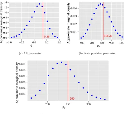
under consideration. . . 110 6.4 Plot of the mode and 95% probability interval for all the three parameters
of the linear model, over time. The actual value of the parameters do not fall within bounds for any of the cases, symbolizing poor performance for our algorithm when used with the crude method. . . 112 6.5 The posterior marginal distribution for each of the parameters are plotted
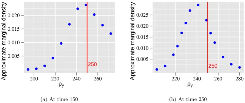
along with the true values given by the red line. Note that INLA is successful in identifying the true value of the parameter for some specific data set from the linear model. . . 114 6.6 Posterior marginal density defined over the grid for the observation
preci-sion parameter ρy as computed by INLA. The true value lies outside the
6.7 Posterior marginal density adding more grid points to the right tail and dropping points at the left tail. Thus from the starting grid provided by the INLA, the grid has moved considerably to accommodate for the true value. . . 115 6.8 Plot of the mode and 95% probability interval for all the three parameters
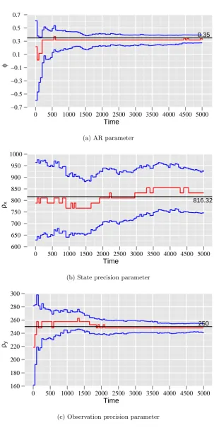
over time for some particular data set simulated from the linear model. The performance of the algorithm is quite good for this particular case. . . 116 6.9 The actual value of the state precision parameter, ρx of the linear model
lies outside the probability bounds after 5000 updates to the posterior dis-tribution. . . 117 6.10 In this example the starting grid does not cover the actual value of the
observation precision parameter, ρy of the linear model. However, the
pos-terior density adds points externally over time to shift and finally the actual value falls within the probability bounds. . . 117 6.11 Plot of the averaged mode and 95% probability interval for all the three
parameters over time. The average is done over all the data sets simulated from the linear Gaussian model. Hence on an average the performance of our approach has been excellent for this particular model. . . 118 6.12 Plot of the mean and 95% probability interval of all the three parameters
over time using particle filter for the linear model. Note that the intervals and the mean merge with each other at around time point 400. . . 120 6.13 The gradual decrease of unique particles of the parameters over time. This
happens since there is no sampling-resampling procedure associated with this filter. . . 121 6.14 Plot of the mean of the three parameters calculated over time using particle
filter, with each trace denoting a certain data set simulated from the linear model. . . 122 6.15 Plot of the average of the mean of the three parameters over time, along
with the average of the 2.5% and 97.5% quantile of the particles, calculated from samples generated by particle filter on the linear Gaussian model. . . . 123 6.16 Box-plot of Mahalanobis distance computed at regular intervals of time for
the two methods implemented for the linear model. The starting box plot on the extreme left of the figure is the Mahalanobis distance computed on the grid provided by INLA, after 25 time points. . . 124 6.17 Coverage proportion for each of the parameter values plotted over time for
6.18 Error bar of log-computation time (secs) of each algorithm plotted against Mahalanobis distance computed for time 500 and 1000 for the linear Gaus-sian model. The limit of the bars are the 25thand 75th percentile respectively.125 6.19 The posterior marginal distribution for each of the parameters are plotted
along with the true values of the parameters for the nonlinear model, given by the red line. INLA has successfully identified the true parameter values in this specific data set simulated from the model. . . 127 6.20 This is an example, where the starting grid provided by INLA is not able to
identify the true value of the parameterφ, for a specific data set simulated from the nonlinear model. . . 128 6.21 Posterior distribution of one of the parameters at different time points of
the algorithm. Note the change in support of the posterior and also the incredible change in shape of the density. . . 129 6.22 Plot over time, of the mode and 95% probability interval for all four
param-eters from the nonlinear model. The performance of SINLA has been good overall, with failure to identify the state precision parameter completely. . . 130 6.23 An example of the sequential algorithm identifying the true value of the
state precision parameter,ρx, from the nonlinear model. . . 131
6.24 Trace plot of the averaged mode and 95% probability interval for all the four parameters from the nonlinear model. The average is done over all the data sets simulated from this particular model. . . 131 6.25 Plot showing mean of the particles generated using SMC, at each time
point for all the data sets simulated from the nonlinear model. Some of the runs have produced divergence, where the trace plot has moved away and continue to do so after several iterations. . . 133 6.26 Plot showing grand mean of the particles for all the parameters of the
nonlinear model along with 95% probability bounds. The particle filter fails to identify the actual value of nearly all the parameters. . . 134 6.27 Box plot of log of Mahalanobis distance for the two methods applied on
the data sets simulated from the nonlinear model. There are many extreme values using SMC, for which the distance is calculated on a log scale. . . 134 6.28 Coverage proportion for each of the parameter values of the nonlinear model
6.29 Error bar of log-computation time for each algorithm applied on the data sets simulated from the nonlinear model, plotted against Mahalanobis dis-tance computed for time 500 and 1000. The limit of the bars are the 25th and 75th percentile respectively. . . 136 6.30 The posterior marginal distribution for each of the parameters of the
non-Gaussian model are plotted along with the true values given by the red line. INLA performs very poorly in identifying the transformed parameters for this specific simulated data set. . . 137 6.31 Good identification of the actual value of the transformed parameter, κ as
seen from the plot of the posterior marginal density, computed using INLA. 138 6.32 Plot of mode and 95% probability interval for both of the transformed
parameters of the non-Gaussian model over time for a certain simulated data set. . . 139 6.33 Plot of the averaged mode and 95% probability interval for both of the
transformed parameters from the non-Gaussian model, over time. The av-erage is done over estimates of the statistics calculated over all the simulated data sets. . . 140 6.34 Plot of the mean of the two transformed parameters of the non-Gaussian
model, over time, with each trace denoting a certain simulated data set. Particle filter is quite successful in identifying the true values of the param-eters. . . 142 6.35 Trace plot of the average of the mean of the two transformed parameters of
the non-Gaussian model. The average has been done over all the data sets simulated from this model. . . 143 6.36 Box plot of log of Mahalanobis distance for the two methods applied on the
data sets simulated from the non-Gaussian model. The values are plotted on a log-scale because of the presence of outliers for the sequential INLA method. It has been observed that our algorithm diverged for a specific simulated data set, resulting in extreme values of the mode. . . 144 6.37 Coverage proportion for each of the parameter values plotted over time for
the non-Gaussian model. We start with plotting the coverage proportion for INLA based on the first 50 observations. . . 145 6.38 Error bar of log-computation time of each algorithm applied on the data
A.1 Plot of the mode and 95% probability interval for all the three parameters over time for the linear model in Example A.1. The actual value of the pa-rameters perfectly fall within the bounds indicating successful identification of the parameter by our approach. . . 154 A.2 Plot of the mode and 95% probability interval for all the three parameters
over time for the linear model in Example A.2. The actual value of the pa-rameters perfectly fall within the bounds indicating successful identification of the parameter by our approach. . . 155 A.3 Plot of the mode and 95% probability interval for all the three parameters
over time for the linear model in Example A.3. The actual value of the pa-rameters perfectly fall within the bounds indicating successful identification of the parameter by our approach. . . 157 A.4 Plot of the mode and 95% probability interval for all the three parameters
over time for the linear model in Example A.4. The actual value of the pa-rameters perfectly fall within the bounds indicating successful identification of the parameter by our approach. . . 158
B.1 Plot over time, of the mode and 95% probability interval for all four pa-rameters from the nonlinear model. The performance of SINLA has been good overall, with failure to identify the theta parameter completely. . . 160 B.2 Plot over time, of the mode and 95% probability interval for all four
pa-rameters from the nonlinear model. The performance of SINLA has been quite poor, with complete failure to identify most of the parameters. . . 161
C.1 Plot of mode and 95% probability interval for both the transformed pa-rameters of the non-Gaussian model over time for the non-Gaussian model presented in Example Appendix Non-Gaussian models. The performance of our approach is very good, considering the fact that it has successfully identified the true values of the unknown parameters for this model. . . 163 C.2 Plot of mode and 95% probability interval for both the transformed
pa-rameters of the non-Gaussian model over time for our non-Gaussian model presented in this section. SINLA has successfully identified the true values of the unknown parameters for this model as is quite evident from the plots. 164 C.3 Plot of mode and 95% probability interval for both the transformed
List of Tables
4.1 Array in which the parameter values and approximate log-posterior values are stored . . . 71 4.2 Updated matrix where the internal grid is being updated. . . 71 4.3 Storage matrix at time tbefore internal points are added. . . 78 4.4 Storage matrix at time t after internal points are added and their
log-posterior calculated using interpolation. . . 79 4.5 Storage matrix at time tbefore external points are added. . . 86 4.6 Storage matrix at time t after external points are added and the
Chapter 1
Introduction
Sequential Bayesian estimation of parameters which do not change over time forms the basis of this thesis. In time series, machine learning and signal processing, there exists a large array of problems which require estimation and forecasting in real time, using noisy observations. In such areas, data is modeled using a dynamic state space model in which estimation of the unknown parameters are necessary. In most applications, however, the parameters of the model are independent of time, and remain fixed (also known asstatic). While some work has been done on estimation of time-dependent parameters, the area of estimation of static parameters in the model requires special attention. Hence, more specifically, this thesis introduces a new approach for static parameter estimation in general dynamic state-space models. This research idea was motivated by a problem involving estimation of signal-power of cognitive radio devices in wireless telecommunications.
1.1
Motivation
The main motivation for this research is to make accurate real-time estimation of unknown parameters in a dynamic state-space model. It started as trying to address a problem related to analyzing signal strength in wireless networks which is an ongoing research under Prof. Linda Doyle in the Center for Telecommunications Value-Chain Research (CTVR) at Trinity College, Dublin. The principal factor in this research is for cognitive radio devices to efficiently analyze the signal in real time and detect the lack of transmission power at a given frequency.
a) some frequency bands are largely unoccupied most of the time; b) some bands are only partially occupied;
c) the remaining bands are very heavily used, causing problems with accessing it.
Thus if communicators use these interleaved and fragmented bands temporally, the spectrum-usage will be more effective and the cost of the spectrum now used will be much lower. A device (inclusive of software) meant for efficient use of the spectrum by exploiting the existence of unoccupied frequency bands (or spectrum holes) would thus assist this new idea. The cognitive radio (Haykin 2005) is such a device and is defined as an intelligent wireless communication system that is aware of its environment and uses the methodology of ‘understanding-by-building’ to learn from the environment and adapt to variations in the input stimuli. The main objectives of such a device are the following:
• highly reliable communication whenever and wherever needed; • efficient utilization of the radio spectrum.
An important objective of cognitive radio is to develop a spectrum accessing system whereby, once the cognitive radio detects a spectrum hole, it will be permitted to transmit at that frequency and make use of the lack of primary user activity.
In order for cognitive radio devices to conform to any specified frequency usage eti-quette, and to ensure they do not interfere at frequencies that are indeed being transmitted upon by other primary users, knowledge of the prevailing radio environment must be con-stantly available. As such, and because any radio environment of interest is likely to be subject to rapid fluctuations due to changes in the power being transmitted along any given frequency, the recordings made by the radio device must be efficiently analysed in real or virtually-real time, and must result in a highly accurate approximation of current frequency usage. This task is more difficult due to the requirement that it be accom-plished in light of residual uncertainty concerning background noise and interference from additional frequency users.
Dynamic state-space models are a rich class well suited in capturing the uncertainty associated with the spectrum along with incorporating the physical properties, which in turn would help in better prediction for signal strength and identifying spectrum holes. We discuss this idea in more detail in the next section.
1.1.1 Motivation for the Statistical Research
Generally, two main styles of statistical modelling can be distinguished for the previously discussed wireless network usage problem. The recorded signal of a single user having a receiver of some kind forms a time dependent data set. On one hand, one can fit a model for the whole data set and estimate the unknown parameters. Classical time series developed by Box et al. (1970) and inference using general state-space models are examples of such inference method. A different methodology for dealing with the dynamic spectrum problem discussed above is processing received data sequentially rather than in a batch and this idea is best utilized through dynamic state-space models approach. Such models are very well suited for providing a solution to the spectrum problem, since prediction will be provided in real time. Two distinct elements are usually unknown in such models. One is the unobserved state process and the other are the parameters associated with both the noise and the state process. Sequential estimation requires speedy inference while maintaining accuracy in estimating the unknowns. A major driving force behind this, is the increase in computational ability which has made the Bayesian approach more popular. In this thesis, we are dealing with sequential Bayesian estimation of these unknowns.
While a lot of research has been done on state estimation, the area of parameter estimation has got much less attention in comparison. Sequential parameter estimation is not straight forward, because not only do they have a non-Gaussian distribution (in general), they also have a strong nonlinear relationship with the observations. This makes Bayesian inference of the model unknowns in real time very complex since one has to achieve both speed up and accuracy.
The key observations noted in the methods discussed above that lead us to this work are the following:
1. There is a need for real time static parameter estimation. Very little work on this problem has been attempted and this problem requires developing a good method-ology which maintains a balance between computation speed and accuracy;
2. Bayesian estimation of parameter by identity would make an easily implementable and efficient algorithm for estimation of static parameters on a grid. Moreover, this idea would also increase the computation speed of the algorithm when compared to sampling based techniques, and
3. In many problems we find that the parameter space is often of low dimension and this allows grid based estimation, which again is very fast and accurate.
These three points form the basis of this thesis. The problems of the category of real time sequential estimation such as the problem of dynamic spectrum discussed in the previous section is an area which demands a solution which is both accurate enough and speedy, and hence fits into this problem.
1.2
Research Contributions
The main research contribution of this thesis is listed below:
• A new real-time parameter estimation method for general state space models has been discussed in this thesis. This new method is inspired from the work of Rue et al. (2009) on the Integrated Nested Laplace Approximation (INLA) for Gaussian Markov random fields (GMRF) and is deterministic, rather than sampling based in nature. The new method is grid based, which can be viewed as an extension to INLA and has been named Sequential INLA (SINLA), even though it is not quite the sequential version of INLA. This thesis provides the algorithm for this method, which is easy to use and also gives examples of its possible usage along with the limitations. There are two advantages to this method which are listed below. • Firstly, the new method can be applied to a diverse range of state space models.
The new method can be implemented on all those models for which INLA can be used and many more as will be discussed in the latter chapters.
parameters. Hence this method has the strength to out-perform most of the existing parameter estimation algorithms, in line with the possible restrictions that we have already mentioned. As far as we are concerned, work on this has not been done earlier.
1.3
Overview of Chapters
The rest of the thesis is organized as follows:
Chapter 2: Time Series and Sequential Estimation
In this chapter we discuss the preliminaries associated with classical time series models and then moves on to general state space models. We also explain the difference between off-line and on-line estimation methods. Classical time series modelling methods like those using Box-Jenkins models namely ARMA, ARIMA etc are given. References to off-line estimation of parameters are also included in this chapter. Parameter and state estimation methods involving state space models, viz. , DLM, Kalman filter and its extensions, SMC and other well known methods are also discussed in greater detail.
Chapter 3: Statistical Methodology
Statistical methods that are used for analysis are detailed in this chapter. This includes a short discussion on classical and Bayesian inference. Since almost all of the modelling is done in the Bayesian framework it receives more attention. The motivational idea for our method is INLA. The assumptions associated with INLA and the construction of the grid for the parameter space has been discussed broadly. Our method has been compared to existing methodologies like MCMC and SMC. Hence the Markov chain theory associated with both these methods and the different algorithms are briefed in this chapter. We also provide a proof of Kalman filter, based on Bayes theorem, at the end to give an idea of deterministic filtering methodology that has been used extensively for both linear and nonlinear models. This is particularly important since all our examples use the Kalman filter or sub-optimal extensions of it.
Chapter 4: Sequential Parameter Estimation in Time series models
which SINLA gives poor inferences.
Chapter 5: Correction to Improve Posterior Density of the Parameters
The sequential parameter estimation methodology, introduced in Chapter 4 can have a problem similar to the degeneracy problem (Doucet, Godsill & Andrieu 2000) in SMC. In this chapter, we provide a correction factor that can be put in the algorithm for complex models with outliers, which is when the problem arises mostly. This correction factor helps in better estimation of the parameters. However this may make the model slow, a reason why it is not used for all the models. We show with an example how the inference is improved with this correction factor.
Chapter 6: Application of Sequential Algorithm to Simulated Examples The developed algorithm, SINLA is applied to different models in this chapter. The performance of the algorithm is being tested with respect to different models with different complexity levels. Static parameters of both linear and nonlinear models and also models with non-Gaussian error are being estimated and their accuracy checked using existing statistical measures. The performance of SINLA has also been compared to SMC and INLA itself, to get a view of the performance accuracy with respect to computation speed. Chapter 7: Conclusion
This is the last chapter which concludes this thesis and provides a short discussion on possible future work related to this method.
Chapter 2
Time Series and Sequential
Estimation
In this chapter, modelling of time series data is discussed in the general setting of classical time series methodology and general state-space models. A short overview of time series methods is provided, followed by generalized state space methods. The state space method is presented both from an engineering and a statistical point of view. Subsequently, both the off-line and on-line estimation techniques used for state-space models are explained. More importance has been given to the one-line estimation technique, better known as sequential estimation and basic examples are used to better understand this methodology. Special emphasis has been given to the Bayesian framework of estimating the unknowns, since our developed method is based on it. Refer to Box et al. (1970) for an insight into the classical time series modelling and Durbin & Koopman (2001) for general state-space models. Sequential inference of state-space models in a linear set up is explained in great detail in West & Harrison (1997). Grewal & Andrews (2011) gives an adequate account of the problems and modelling techniques from an engineering standpoint.
2.1
Time Series and Forecasting
Much of statistical methodology deals with models in which the observations are assumed to be independent. In planned experiments, techniques likerandomization are introduced to ensure that independent observations are collected, since dependence is considered a nuisance for construction of the model and makes inference a very complex exercise. How-ever, several fields of research like business, economics, engineering and natural sciences produce data that are dependent and are ordered. Such observations are calledtime series
data and main interest lies in studying the nature of the dependence. Primary interest often lies in prediction orforecasting future values from current and past values.
time. Let Yt be the random variable at time t, denoting some time-dependent physical
process, andYt−1,Yt−2, . . . be that from previous time points. The basis of investigation for different scientists or economists then becomes prediction of the values of the physical process under consideration at some future time point t+l, where l >0 and to find an estimate ˆYt+l.
The classical time series technique uses the Box and Jenkins’ methodology to model and forecast time series data. A subsequent development wasstate space modelling which is considered to be more generalized for treatment of a wider range of problems that include both non-stationarity and non-Gaussian property. The rigidity of the classical models can be avoided by the structure of the state space models. This is mainly because state space models allow a natural interpretation of a time series as the result of several components, namely, trend, seasonality and regression covariates. Moreover, the classical ARMA models can be shown to be a special case of the state space approach (Durbin & Koopman 2001). The Bayesian framework has been used in both types of inference and prediction ((Monahan 1983) and (West & Harrison 1997)). This will be discussed in more detail in the future sections of this chapter.
Time series inference is generally of two different types. A dynamic model methodology does real-time inference as observations are recorded sequentially in time. The problems of estimation and forecasting are solved by recursively computing the conditional distribution of the quantities of interest, given the available information (Arulampalam et al. 2002). A very important feature of this method is that past data need not be stored as only new data are used to update the conditional posterior. A static model methodology on the other hand is not a recursive procedure. At any given point in time, it uses all the data to estimate the parameters (Brockwell & Davis 2002) and data needs to be stored for this purpose. Hence it makes use of all the data to model and forecast in a static framework.
2.2
Time Series Models
In this section we discuss classical modelling of time series observations as proposed by Box et al. (1970). This discussion includes model fitting and estimation of model parameters. This is followed by discussing state space modelling and we explain why this modelling technique is more generalized. Finally we discuss the application of state space models in dynamic inference of real time data.
2.2.1 Classical Time Series
The most basic model used in time series is the linear additive model, also known as the classical decomposition model:
yt=Tt+St+t t= 1,2, . . . , n.
Here, Tt is a slowly changing component called the trend, St a periodical component
with a fixed period referred to as the seasonal component and t is the random error
component, assumed to be Gaussian. The error component needs to be stationary for many inference methods under classical time series to work successfully. This assumption, if not true, requires transformation on the data to ensure stationarity. In many applications, these components are multiplicative (Cowpertwait & Metcalfe 2009) and the model is converted to the additive model by a logarithmic transformation. The general framework for studying stationary processes is based on linear time series models, namely Box-Jenkins autoregressive moving-average (ARMA) models (Box et al. 1970). A process {Yt} is said
to be anARMA(p,q) process with meanµif{Yt−µ}is anARM A(p, q) process denoted
as
φ(B)Yt=θ(B)Zt,
whereφ(·) andθ(·) are pth and qth degree polynomials
φ(x) = 1−φ1x− · · · −φpxp,
and
θ(x) = 1−θ1x− · · · −θqxq.
B is the backward shift operator (BjXt = Xt−j, j = 0,±1,· · ·). The time series {Yt}
is said to be an ARMA model of order (p, q), where p is the number of AR parameters and q is the number of MA parameters. Zt is a random component which follows a
Gaussian distribution with mean 0 and variance σ2. It is important to keep in mind that an essential part of this definition is that Yt needs to be stationary, for which the
the equation and also make sure that the solution is unique. Determining the appropriate model involves several steps. Determining the values of (p, q), also known as order selection is done using graphical procedures like the Auto-correlation function (ACF) plot or the Partial Auto-correlation (PACF) plot. A variety of goodness of fit tests or minimization of AIC statistic (Brockwell & Davis 2002) are other methods of determining the order of time series model.
A generalization of the ARMA class of models is done by modelling nonstationary time series. Autoregressive integrated moving-average (ARIMA) processes provide this generalization. This is done by introducing an extra non negative parameter into the model, known as the difference parameter (d). A time series,{Yt} is anARIMA(p,d,q)
process if Xt := (1−B)dYt is a causal ARMA(p,q) process. The definition just states
that the process reduces to an ARMA series when differenced finitely many times. The difference operator (d) also needs to be determined while the model selection is done. A further extension to ARIMA models is the seasonal ARIMA (SARIMA) model. Once differencing is applied to the data in these models, the analysis is same as that of ARMA models. The only unknown component is the differencing parameterd.
2.2.2 Inference and Prediction for ARIMA
Maximum likelihood estimation has been the most popular estimation technique for the parameters φ = (φ1,· · · , φp), θ = (θ1,· · ·, θq) and σ2. Some preliminary estimation
techniques like Yule-Walker estimation or Burg’s algorithm are used to get good initial values (Brockwell & Davis 2002). From an application point of view, the most important question one asks is regarding prediction; prediction of series h-steps ahead in time where we have data until time t. Thus one would be interested to make predictions about Yt+h
given that we have some data y1,· · · , yt, for some h > 0. Durbin-Levinson algorithm
and theInnovations algorithm (this is applicable to all series with finite second moments, regardless of stationarity) (Brockwell & Davis 2002) are usually used for predicting h-step ahead. Once reduced to ARMA models, all these estimation and prediction methods can also be used for ARIMA or SARIMA models. Note that prediction is usually carried out by using extensions of the methods developed for ARMA models.
simulate from intractable joint distributions. There were of course other problems, for ex-ample initial applications debated over the choice of prior, a primary exex-ample of which is the controversy over the choice of prior for the coefficients of models (Steel 2008). Box and Jenkins devoted a section to Bayesian estimation and proposed the use of Jeffrey’s prior (Jeffreys 1961). Subsequently, a ‘fully’ Bayesian analysis of ARMA models is provided by Monahan (1983). For a very good source of extensive study of Bayesian time series, the interested reader should look into Prado & West (2010).
2.3
State space models
State space representations have had a profound impact on time series analysis in the last decade or so. This is an extremely rich class of models for time series, including and going well beyond the linear models like ARMA and the variations thereof. The rigidity of the classic time series models are avoided by allowing the trend and seasonal components to evolve randomly rather than deterministically as was the case of the classical decomposi-tion models (Brockwell & Davis 2002). In other words, state space models consider a time series as the output of a dynamic system perturbed by random disturbances. This struc-ture allows a natural interpretation of the time series in terms of the components. At the same time, these models have an elegant and powerful probabilistic structure, allowing a natural treatment using the Bayesian approach. These models can be used to model both univariate and multivariate time series and include non-stationarity and irregularity in its formulation. State space models are very widely used in economics, biology, sociology, engineering and several other fields.
Real world time dependent processes produce observable outputs which can be char-acterized either in discrete time e.g. digital signals, characters from a finite alphabet, or continuous time e.g. speech samples, temperature measurements etc. In the state space approach it is assumed that there is a hidden system Xt∈Rnx,t∈N, also known as the
latent variable. It is better known as the state process and it has an initial probability
PX0(x0) at time t = 0. It is further assumed that the state process evolves over time t as a first order Markov process (the Markov property is discussed in detail in the next chapter) according to the transition densityPXt|Xt−1,Θ1t(xt|xt−1, θ
1
t), whereθ1t represents
a set of parameters. The observations are denoted by Yt ∈ Rny and are assumed to be
conditionally independent given the states and some set of parameters Θ2t. They are gen-erated from the conditional probability density PYt|Xt,Θ2t(yt|xt, θ
2
t). This is also known
as the measurement process. It is of course possible that some of the parameters do not depend on time. As already discussed in Chapter 1, such parameters are known as static parameters and denoted by θ. For simplicity, we denote all the unknown parameters as
described by
P(x0|θ), (2.3.1)
P(xt|xt−1, θ) t≥1 and (2.3.2)
P(yt|xt, θ) t≥1. (2.3.3)
The probability distributions can be continuous or discrete, andtis strictly discrete. This pattern is best illustrated by the followingdirected acyclic graph (DAG):
yt‐1 yt yt+1
time
xt‐1 xt xt+1
P(yt | xt)
Figure 2.1: DAG representing the general state space model where the parameters are not shown.
An equivalent representation of the above model is the general state space model, in which the state variable is the same as the latent variable. The representation for a continuous time process is
∂xt
∂t =gt(xt−1,wt, θ2), (2.3.4)
yt=ft(xt,ut,vt, θ1), (2.3.5)
where in Equation (2.3.4)gt: Rnx×Rnw×Rnθ2 →Rnx is a possibly nonlinear function,wt is the system/state error and nx,nw and nθ2 are the dimensions of state, state error and parameter vectorθ2, respectively. In Equation (2.3.5),ft: Rnx×Rnu×Rnv×Rnθ1 →Rny is also a possibly nonlinear function,ut is some covariate process that is fully known and ny,nu,nv andnθ1 are the dimensions of measurement process,ut, the measurement error and parameter vector θ1, respectively. The likelihood is fully specified by f, vt and θ1,
while the continuous transition densityP(xt|xt−1, θ2) is completely specified bygandwt.
We denote byθ={θ1, θ2}.
and is of the following form:
yt=f(xt,ut,vt, θ1), (2.3.6) xt=g(xt−1,wt, θ2). (2.3.7)
The state-space model, together with the prior distributions of the hyperparameters and the system states, defines stochastically how the system evolves over time and how we inaccurately observe the hidden state process. We provide an example here from the cognitive radio example we discussed in Chapter 1. For this purpose, recordings were analysed from a signal transmitted by the Three Rock Antenna south of Dublin. The following state space model was fitted to the collected data:
yt=xt+vt vt∼ N(0, σ2u), (2.3.8)
xt= (1 +φ)xt−1−φ xt−2+wt wt∼ N(0, σ2w). (2.3.9)
Parameter φ and the variance parameters σ2
u and σ2w are unknown and need to be
esti-mated. This is an example of a discrete state space model, where we assumed that there is an underlying process,xtwhich signifies the true signal whereas the data we record are
noisy realisations of the true process. A plot of 100 recording of the data along with the fitted filtered level of the state processxtof the above model is shown in Figure 2.2 It can
−0.6
−0.4
−0.2
0.0
0.2
0.4
● ● ● ●● ● ●●●● ● ● ●● ●●● ● ●● ●●●● ● ●●●●●● ● ●●● ●●● ●●●● ●●●● ● ● ●● ● ● ●●●● ●●● ● ● ● ●●●●●●● ●●●●● ●●●●● ● ●●●●●● ●● ●● ●● ●●● ●● ● ● ●0
20
40
60
80
100
Time
Recording of signal (dB)
●
Data
[image:31.595.135.478.444.695.2]Filtered level
Figure 2.2: Fit of filtered levelxt over data recorded from Three Rock antenna, south of
Dublin. The fit is done using a state space model with three unknown parameters.
have fitted well to the data. If we try to fit an ARMA or ARIMA model though, the model will be difficult to interpret in terms of the physical process in hand. It is easy to see the advantages one has when fitting a state space model, not only in terms of interpreting the model but also in terms of construction of the model. The rigidity of ARMA models is absent since one can go on adding layers to the model, with each layer depicting a physical process. This is discussed more broadly in the remaining part of this section.
State space techniques have several advantages over the Box-Jenkins time series mod-els. The model building process is very structural and hence methodical. The different components of the classical model, such as trend or seasonal variations can be modelled separately and then put together to form a single state space model. Extra effects of explanatory variables are also easy to put in the same model. The following equations provide an example to explain what we mean:
yt=Tt+st+ut+vt, Tt=Tt−1+wt,
st=st−1+zt,
where one can think of Tt, st and ut as trend, seasonal and fixed covariate input
respec-tively. vt, wt and zt are the error components. In addition to this structural formation,
they are also very general, in the sense that they comprise all ARIMA models (Durbin & Koopman 2001). Multivariate observations can be handled by straightforward extensions of univariate theory. It is also possible to allow for missing observations. Furthermore, because of the Markovian structure of state space models, the calculations needed to im-plement them can readily be imim-plemented in recursive form. The models in which the recursive Bayesian technique is applied are generally known as dynamic models. These models enable large data sets to be handled without a huge increase in computational burden, since these methods work sequentially and it is not necessary to store the data. Thus assuming we have some data setY1:T :Y1,· · ·, YT; at timeT, dynamic models would
only requireYT to make any inference about the parameters or state process. Box-Jenkins
type models on the other hand will need to store the whole data set,Y1:T. AsT becomes
large, computational issues set in and the algorithm fails. This idea will be discussed in more detail in the next section.
2.3.1 Dynamic Models
A dynamic model is a forecasting model which can be expressed in a recursive form. Dy-namic or sequential inference is necessary when one needs to update the posterior in real time, fromP(xt|y1:t−1) toP(xt|y1:t). It is well known that state space models are ideal for
linear Gaussian models produce exact inference, which requires updating the first two mo-ments at each time t, this is not the case for nonlinear or non-Gaussian models. Hence dynamic models are generally divided into linear models and nonlinear/non-Gaussian mod-els, the estimation procedures of which are treated differently. We will be describing the two different types of models in the following sections.
2.3.2 Dynamic Linear Models
The most widely known and used subclass of dynamic models is known as theNormal Dy-namic Linear Models, more popularly known asDynamic Linear Models (DLM) (West & Harrison 1997). The fundamental principles used by a forecaster in dealing with problems through dynamic linear models comprise:
• sequential modelling;
• structural state space model;
• probabilistic representation of the parameters and forecasts.
These properties form the basis of any sequential inference algorithm.
The general DLM for a vector observationYtof the time seriesY1,Y2, . . . is given by:
yt=F
0
txt+vt vt∼ N(0,Vt), (2.3.10)
xt=Gtxt−1+wt wt∼ N(0,Wt), (2.3.11)
where for each timet:
1. ytrepresents a (n×1) measurement process;
2. xtrepresents a (p×1) state process;
3. Ftrepresents a (p×n) matrix, probably representing explanatory variables;
4. Gtrepresents a (p×p) matrix, also known as the evolutionary matrix;
5. Vt represents a (n×n) covariance matrix;
6. Wt represents a (p×p) covariance matrix.
Att= 0, the initial information is that the mean and variance ofX0|Y0 are assumed to be known to be m0 and C0 respectively. It is further assumed that the error sequences vtand wt are uncorrelated with each other in all time periods and uncorrelated with the
initial stateX0, i.e.E(vsw
0
t) = 0, for all sand t= 0,1,· · ·; and E(vtX
0
0) = E(wtX
0
has been discussed in Nieto & Guerrero (1995). Serial correlation of errors can also be allowed for generalization of the problem, a partial treatment to which has been provided by Gelb et al. (1974). In real life situations, the elements Ft, Gt, Vt and Wt can be
assumed to be unknown and dependent on a vector of parameters θt, which need to be
estimated.
2.3.3 Nonlinear/Non-Gaussian Models
Several physical systems, such as stochastic volatility are better modeled as nonlinear or non-Gaussian or both. There are situations, for example data generated from ecological process which cannot be modeled using Gaussian distribution, even after transforma-tions. Here it is more plausible to have non-Gaussian distribution, for example a skewed distribution (Fr¨uhwirth-Schnatter 1994). Also with discrete data, approximations using continuous Gaussian distributions may be inappropriate. Binary series occur as indicators of presence or absence of sequence of events, say for example daily rainfall indicators. Generalized models of this type are represented as the equations stated in (2.3.6) and (2.3.7), where the functions f(·) and g(·) are possibly nonlinear and the errors vt and
wt are possibly non-Gaussian. Such models make filtering, smoothing or prediction much
more complex since the posterior integrals are usually not obtainable in closed form, as in linear Gaussian models. Since analytical solution is hard to find, numerical methods are being developed to solve for these models (Arulampalam et al. 2002).
2.4
Inference for State Space models
In sequential estimation, a statistician is mainly interested in the three concepts of filtering, smoothing and prediction.
Filtering is the recovery of information, at time t, of the state process from the noisy observations up to time t. So if Xt denotes the non-measurable state process at time t
as defined in Equation (2.3.7), and Y1:t=Y1,Y2, . . . ,Yt be the noisy observations until
and including time t, then we are interested in the distributionP(xt|y1:t), also known as
the filtering density. If there are unknown parameters, sayθ, then one might be interested in either P(xt|y1:t, θ) or the unconditional (on θ) distribution P(xt|y1:t). The latter is
using the following integral:
P(xt|y1:t) = Z
P(xt|y1:t, θ)P(θ|y1:t) dθ. (2.4.1)
Smoothing differs from filtering in the sense that observations both before and after timetcan be used to get information about the state at timet. This means unlike filtering, which tries to infer the distribution of the state in real time, there is a delay in smoothing regarding the inference. But this disadvantage can be remedied by the fact that since more observations are used, the inference will be more accurate. In smoothing we are actually interested in the distribution P(xt|y1:s) where s > t. This can be explained intuitively
by how the human brain tackles hastily written handwriting (Anderson & Moore 1979). When one word is difficult to interpret, words before and after it are used for understanding the difficult word.
Prediction is the same as forecasting. As explained earlier in Section 2.2.2, h-step ahead predictions,P(yt+h|y1:t) are to be calculated. In time series modeling, the area of
prediction is the one in which statisticians are mostly interested in. Ample examples of prediction are available in literature (Durbin & Koopman 2001).
The joint posterior P(x1:T |y1:T) is also of interest, but it is not always possible to
calculate it directly like the filtering process. The following decomposition is useful (Doucet & Johansen 2009):
P(x1:T|y1:T) =P(xT |y1:T) T−1
Y
t=1
P(xt|xt+1,y1:T),
=P(xT |y1:T) T−1
Y
t=1
P(xt|xt+1,y1:t). (2.4.2)
It is possible to further break the termP(xt|xt+1,y1:t) in (2.4.2) down as
P(xt|xt+1,y1:t) = P
(xt+1|xt)P(xt|y1:t) P(xt+1|y1:t)
. (2.4.3)
All the terms in (2.4.3) are computed using either the model equations or the filtering densities. Note that all the filtering and prediction densities computed up to T need to be stored for the calculation of Equation (2.4.2). It also possible to obtain a recursive formula for the joint posterior density (Doucet et al. 2001),
P(x1:T |y1:T) =P(x1:T−1|y1:T−1)P
(xT|xT−1)P(yT |xT) P(yT|y1:T−1)
. (2.4.4)
The denominator term in (2.4.4) is not easy to compute, but is a constant with respect toX1:T. The rest of the terms can be computed from sequential filtering equations. As
the different methods developed in this thesis are discussed, it will be clear which of these decompositions can be used under what circumstances.
which introduces the famousKalman filter. Numerous extensions of Kalman filters exist, each of which tries to improve on the fundamental idea by solving for nonlinear and/or non-Gaussian models. A relatively new but more general class of numerical methods are the
Sequential Monte Carlo algorithms. Other forms of smoothing and estimation techniques like EM algorithm or Expectation Propagation can also be used. The interested reader should look into Durbin & Koopman (2000) and Shumway & Stoffer (1982).
2.4.1 Kalman Filter
Kalman (Kalman 1960) developed a linear filter which produces an estimate by minimizing the conditional mean square error E[ xt−xˆt)T[(xt−xˆt)|y1:t
, where ˆxt is the estimate
ofxt|y1:t. The Kalman filter is the optimum filter in the class of linear filters as given in
Equations (2.3.10) and (2.3.11), in the sense that it is the minimum mean squared error estimator (MMSE). The Kalman filter propagates the first two moments of the distribution of Xt|Y1:t. An interesting feature of this filter is that the model has to be linear while
the errors can be non-Gaussian as has been shown in Kalman (1960). So derivation and the working principle for this filter works even if we drop the distributional assumption in Equations (2.3.10) and (2.3.11).
Let us assume at timet−1, the mean ¯xt−1|t−1 and variance Pt−1|t−1 ofXt−1|Y1:t−1 are known. The Kalman filter updates to the moments when new data Yt arrive, are
shown by the sequential equations below:
1. Prior mean and variance of Xt|Y1:t−1:
¯
xt|t−1 =Gtx¯t−1|t−1, (2.4.5) Pt|t−1 =GtPt−1|t−1GTt +Wt. (2.4.6)
2. 1 -step ahead forecast:
¯
yt|t−1 =FTtx¯t|t−1, (2.4.7) Qt|t−1 =FTtPt|t−1Ft+Vt. (2.4.8)
3. Posterior mean of Xt|Y1:t:
¯
xt|t= ¯xt|t−1+Kt(yt−y¯t|t−1), (2.4.9) Pt|t=Pt|t−1−KtQt|t−1KTt, (2.4.10)
Kt=Pt|t−1FtQ−t|1t−1.
Kt is known as the Kalman gain. It ensures that the posterior means and covariances
time.
The convergence of the Kalman filter depends on the dual concept ofobservability and
reachability. We would not be providing the formal definitions for them (for more de-tails see Walrand (2005)), but only explain their implications on the filter. Reachability ensures convergence of the filter. The observability condition guarantees that the estima-tion error remains bounded. These condiestima-tions ensure asymptotic stability of the filter, i.e. limt→∞Pt|t → P¯ and limt→∞Kt → K, for some limiting values P¯ and K (West &
Harrison 1997).
West & Harrison (1997) provides detailed proof of derivation of Kalman filter using two different methodology. Standard Bayesian calculations are used to deduce the posterior mean and variance of the filtering and prediction density. A second method uses the more intuitive properties of additivity, linearity and distributional closure properties belonging to a Gaussian distribution, where the model has Gaussian distribution for the error terms and state process at time 0,X0|Y0.
2.4.2 Extensions of the Kalman Filter
In the previous section, we have mentioned that the Kalman filter, ideally, can be used for linear models with non-Gaussian errors. While implementing it for non-Gaussian errors, however, it is possible only if one could have closed form expressions for estimates of:
¯
xt|t−1 =E(xt|y1:t−1), (2.4.11)
and
¯
xt|t=E(xt|y1:t). (2.4.12)
Thus the theoretical solution for the filter is more of a conceptual kind and cannot always be determined analytically in practice. For the observation vector originating from an exponential family distribution, conjugate methods exist, the predictive density
P(Yt|Y1:t−1) and the filtering densityP(Xt|Y1:t−1) can be analytically shown to be same
2.4.2.1 Extended Kalman Filter
The Extended Kalman Filter (EKF) gives an approximation to the optimal estimate (Haykin 2001). It does so by linearizing the nonlinear model around the last state es-timate. So rather than propagating the nonlinearity, the EKF considers, at each iteration, a linearization of the nonlinear dynamics around the last predicted and filtered estimates of the state, and for the new linearized dynamics, it uses the Kalman filter. The state space model used with the EKF is given as:
yt=f(xt,ut) +vt, vt∼ N(0,Vt), (2.4.13)
xt=g(xt−1) +wt, wt∼ N(0,Wt), (2.4.14)
wheref(·) andg(·) are nonlinear functions.
As before, we assume at timet−1, the moments ¯xt−1|t−1 and Pt−1|t−1 are known. The filter dynamics with respect to the general equations are as follows:
1. Prior mean and variance of Xt|Y1:t−1:
¯
xt|t−1 =g(¯xt−1|t−1,ut), (2.4.15)
Pt|t−1 = ˆGtPt−1|t−1GˆTt +Wt. (2.4.16)
2. 1 -step ahead forecast:
¯
yt|t−1 =f(xt−1), (2.4.17)
Qt|t−1 = ˆFtPt|t−1FˆTt +Vt. (2.4.18)
3. Posterior mean of Xt|Y1:t:
¯
xt|t= ¯xt|t−1+Kt(yt−y¯t|t−1), (2.4.19) Pt|t=Pt|t−1−KtFˆtQt|t−1KTt, (2.4.20)
Kt=Pt|t−1FtQ−t|t−1 1,
where,
ˆ Gt=
∂g(x)
∂x
x=¯x
t−1|t−1
,
ˆ Ft=
∂f(x)
∂x
x=¯xt|t−1
.
It is obvious that the EKF utilizes the first term of the Taylor’s series expansion of the nonlinear functionsf andgto estimate ˆFtand ˆGt, respectively (Arulampalam et al. 2002).
would expect these filters to do well in high signal-to-noise ratio (SNR) situations. It is easy to see that high SNR essentially implies low measurement error, which in turn means accurate measurement resulting in large reduction in estimate’s uncertainty. It can be shown that asSN R →0,K →0, which means no correction to the posterior means and variance in Equations (2.4.19) and (2.4.20).
Several variations to the EKF have been proposed to improve its performance and these methods fundamentally try to relax some of the assumptions made in EKF. One can include higher order terms of the Taylor’s series expansion of the nonlinear terms. A filter which includes two terms from the Taylor series is known as a second order EKF
(Arulampalam et al. 2002). However these extensions come with the price of higher com-plexity and increased computation, which particularly is a problem for higher dimensional systems. Also there are other nonlinear filters like theGaussian sum filter (GSF), which uses a finite sum Gaussians and in the process involve a collection of EKF for each of the approximate Gaussians. This the main reason why GSF is more powerful than a single EKF Terejanu et al. (2011).
2.4.2.2 Unscented Kalman filter
There exist a number of derivative-free filters which have been developed to improve the performance of the EKF. These include the Unscented Kalman filter (UKF), the Cen-tral Difference filter (CDF) (Ito & Xiong 1999) and the Divided Difference filter (DDF) (Nørgaard et al. 2000a,b). It can be shown that the latter two are equivalent Lefebvre et al. (2004). These filters usually outperform EKF at an equal computational complexity of O(n3), where . A careful analysis of Taylor’s series expansion of the nonlinear func-tions, shows that both UKF and CDF are essentially the same. Both filters calculate the posterior mean in exactly the same way. The only difference lies in the form of approx-imation to the posterior covariance. The CDF ensures positive semi-definiteness of the posterior covariance matrix as opposed to the fact that UKF may produce non-positive semi-definiteness.
Unlike EKF, the Unscented Kalman Filter does not make any approximation to the nonlinear process (Julier & Uhlmann 1997, Julier et al. 1995). It uses the “true” nonlinear system and the only approximation is done on the distribution of the process. The non-linearity is propagated through deterministically chosen points which attempt to capture the “true” mean and covariance of the variables. The posterior mean and covariance are also calculated up to second order using these chosen points.
The procedure of choosing points is being shown in the following equations: X0 = ¯xt−1|t−1
Xi = ¯xt−1|t−1+
q
(p+λ)Pt−1|t−1
i i= 1, . . . , p
Xi = ¯xt−1|t−1−
q
(p+λ)Pt−1|t−1
i i=p+ 1, . . . , p
Sigma
Points, (2.4.21)
W0m = p+λλ
W0c = p+λλ + 1−α2+β
Wim =Wc
i = 2(p1+λ) i= 1, . . . ,2p
Weights, (2.4.22)
and
λ=α2(p+κ)−p.
The p
Pt−1|t−1
i in (2.4.21) is the i
th row or column of the matrix square-root of
Pt−1|t−1. The square root of matrix is performed by well known linear algebra tech-niques, for e.g. Cholesky decomposition or QR decomposition Merwe & Wan (2001).
Two different types of weighting sequence are explained in (2.4.22). It will be seen