Active noise reduction in double panel structures : decentralized adaptive feedforward control

(1)

MASTER THESIS

ACTIVE NOISE REDUCTION

IN DOUBLE-PANEL

STRUCTURES:

DECENTRALIZED

ADAPTIVE FEEDFORWARD

CONTROL

Jurgen Kalverboer

DEPARTMENT OF ELECTRICAL ENGINEERING SIGNALS AND SYSTEMS GROUP (SAS)

EXAMINATION COMMITTEE Dr.ir. A.P. Berkhoff Jen-Hsuan Ho, MSc. Prof.dr.ir. C.H. Slump Ir. E.R. Kuipers

DOCUMENT NUMBER SAS – 2012-012

(2)

(3)

Abstract

In this thesis an adaptive harmonic decentralized feedforward controller is implemented on an experimental setup. The experimental setup consists of a double-panel structure which is mounted on top of an acrylic box with thick walls. In this box a speaker is installed which can produce

disturbance signals. On each panel of the double-panel structure five actuator sensor pairs are installed which are controlled and observed by their own decentralized controller .The goal of this thesis is to minimize the sound transmission of the double-panel structure. The damping of the panel is increased by adding a low-authority feedback controller. The disturbance signal will contain only a few deterministic frequency components. Each frequency component is processed independently, by the harmonic decentralized controllers on the panels.

The stability and convergence rate of decentralized feedforward control is analysed. In simulations it is demonstrated that a decentralized controller can reduce the noise transmission of the structure. There are multiple feedforward control configurations possible, for example, one strategy might only control the incident panel. The most noise reduction is obtained by controlling only the radiant panel. This configuration can reduce the sound pressure level above the panel by 10 to 20 dB for frequencies below 250 Hz. Above this frequency almost no reduction of the disturbance signal is possible.

The addition of feedback control improves the robustness of the system. It reduces the cross-coupling between the decentralized controllers. There are also multiple feedback control configurations possible. The combination of feedback pressure speakers in the cavity and

decentralized feedforward control of the radiant panel reduces the disturbance signal the most in the simulations. In practise this configuration could not be tested, because the pressure speaker feedback controller has not yet been realized.

For optimal control of the double-panel structure the transfer functions between all actuators and sensors in the system must be known. Therefore, a system identification technique is developed. This technique uses the computational components available in the decentralized controllers. The

(4)

1

1 Introduction

This introduction chapter starts with a literature survey of aircraft noise and active noise control. After this survey the research questions are formulated and the ultimate goal of this thesis is presented. This introduction concludes with an outline of the content of this thesis.

1.1 Aircraft noise

Aircraft noise is a major problem for residents near airports. However, also people inside an aircraft get disturbed by the noise the engines produce. The interior noise in an aircraft is mainly produced by two external sources, the fuselage boundary layer and the aircraft propulsion system. In Figure 1 these disturbances are illustrated. The boundary layer noise is generated by movement of the fuselage wall. This wall moves through the outside pressure fluctuations produced by wind and turbulence. This noise is difficult to reduce because it has a stochastic broadband disturbance, for which no time advanced reference signal is available.

Figure 1 Aircraft noise.

Currently most passenger aircrafts are equipped with jet engines which produce broadband noise. An advantage of jet engines is that they produce less noise at the lower frequencies than propeller propulsed aircrafts [1]. The noise generated by a propeller engine contains a few specific frequency components which are equal to the blade passage frequency (BPF) of the propeller and some of its higher harmonics [2]. In Figure 2 the power spectrum in the cabin of a propeller propulsed aircraft is shown.

(7)

4

Figure 2 Noise in the cabin of a propeller propulsed aircraft.

1.2 Active noise control

Passive control is the traditional method to reduce the sound pressure at a given location. This technique uses an object that will absorb the radiated power of the disturbance source. The wavelength of the noise source must be small compared to the dimensions of the power absorbing object to well function. So this type of noise control works best for high frequencies [3] [4]. For lower frequencies you need larger damping objects which have a larger mass. For fuel efficiency, airplanes have to be as lightweight as possible so this is an unwanted feature. There are also more advanced passive control techniques such as for example a Helmholtz resonator. A Helmholtz resonator can increase the acoustical damping level inside a cavity between two plates. Simulations have shown that this can result in an overall improvement of 8dB in the 50-150 Hz range [5].

The other newer method, active control, uses secondary sources which generate a field that will interfere with the field produced by the primary noise source. This field will cancel the primary field, resulting in a reduced sound pressure. If the secondary sources are placed within half a wavelength of the disturbance signal of the primary source in all directions the field will be cancelled by a considerable amount [6] [7]. Although in most applications a similar setup is not possible, still active noise control performs well, especially at low frequencies. The main advantage compared to passive control is that no heavy objects are required for the reduction in sound pressure.

ANC and ASAC

(8)

5

The ASAC method uses a vibrating plate to reduce the transmission of the disturbance source. On this plate actuators and sensors are integrated so that the vibration of the plate can be observed and controlled. By controlling the vibration of the plate the sound transmission through the plate can be reduced. This simplifies the control problem to a two dimensional problem, because only the surface of the plate needs to be controlled.

A vibrating panel radiates with a set of structural modes. Each mode has a sinusoidal component in both directions of the panel. The spatial frequencies of these modes are dependent on the

dimensions of the panel. The radiation of sound of each mode is dependent on the amplitudes of all modes. For some vibration patterns the air in front of the panel can transfer from one side of the panel to the other. Such patterns will not radiate much sound, only vibration patterns that have a net volumetric component will produce a significant amount of sound [9]. The far-field sound radiation of a plate can thus be estimated by measuring the net volume velocity of the panel. The lower modes of the panel are the most efficient radiation modes [10] [11] [12].

Double panel structures can be used as noise insulators. In general they perform better than single panel structures. However, at low frequencies around the mass-air-mass resonance (double structures resonance) they perform worse than single panel structures. In the past years many techniques have been developed to solve this problem. These techniques can be classified in active control and passive control [5].

Tonal and broadband disturbances

The tonal disturbance signal produced by the propeller engines contains only disturbances at a few harmonics. For these different harmonics a separate control filter, a harmonic controller, can be implemented. A harmonic controller measures only the error of that specific harmonic. It is advised to use an adaptive control filter for deterministic tonal disturbances. Because, the transmission from the disturbance source to the error sensor may change due to environmental changes [7]. An adaptive control filter can react on the phase and the magnitude variations of the disturbance signal so that the error is minimalized.

If the disturbance source produces a broadband disturbance signal the above mentioned method is not suitable. The separate control filters will interfere with each other, and abrupt phase changes cannot be realised. In this case only a single filter for the entire spectrum can be used. This filter must be causal, which will limit its performance [7]. Implementing the controller in the frequency domain will reduce the computational complexity. The convergence speed of the adaptive algorithm is similar to the time-domain solution.

Adaptive feedforward control

The simplest adaptive algorithm is the steepest descent algorithm. This algorithm is implemented in the frequency domain, it adjusts the in-phase and quadrature components of the single tone signal fed to the secondary sources [13]. There are other adaptive methods available such as Newton’s algorithm or recursive least squares. These algorithms may have better convergence behaviour under certain circumstances. However, these methods have higher computational requirements [14] [7].

(9)

6

of the cost function with respect to the control effort. Every eigenvalue of the Hessian matrix is related to a mode of the system. Every mode has its own power and convergence rate. The speed of convergence of a mode is determined by the magnitude of the eigenvalue. Slow modes require an excessive high control effort. To limit the required effort a control effort weighting function can be added to the cost function, which will increase the eigenvalues of the system. Modes for which the eigenvalues are much smaller than the effort weighting parameter will not converge. Their

contribution in the error signals of these modes will not be removed [13] [6].

The adaptation rate of a steepest descent adaptive filter is dependent on the convergence coefficient of the filter. If the convergence coefficient value is too small, the algorithm will stop before the minimum error is reached. On the other hand, if this value is chosen to large the system will become unstable. For SISO systems the convergence coefficient is limited by the time delays in the

cancellation paths of the secondary sources (23) [6]. For MIMO systems this is limited by the eigenvalues of the modes [13]. Faster adaptation does not result in better system performance, it usually decreases it. During fast adaptation unexcited system modes may be triggered, and this can lead to a performance decrease. A large sensor noise can also excite these unreferenced signal modes [15].

Model errors in adaptive controllers may lead to unstable systems or increased error signals [16]. By adding a bounded uncertainty region to the complex plant response optimal control can be obtained without making the system unstable [17].

Centralized and decentralized control

In comparison to centralized control, decentralized control is more scalable, however since each controller is designed based only on local sensor information (rather than all available sensor data), the performance is usually not as good as with a centralized control system.

For the communication between the centralized controller and the error sensors is a great deal of wiring required (see Figure 3). Not all applications will have the required space for this wiring. Another disadvantage of a centralized controller is the amount of processing power required to update all the controller coefficients. This also requires a very complex model of the entire system. And a single defect actuator may result in a significant decrease of performance [18].

Figure 3 Centralized control and decentralized control

In a decentralized system there is only feedback between every actuator sensor pair (see Figure 3). However, all actuators may excite every sensor. The intuitive condition for stability for a

decentralized system requires that the direct coupling in the physical system is larger than the

(10)

7

coupling. A system can thus only be stable if a sensor is closer to the actuator controlling it than to any other actuator. However, this is not a necessary condition for stability. The real upper limit of stability is found by looking at the eigenvalues of the product of the plant transfer matrix and the estimate of the plant transfer matrix which contains only the direct coupling components. If the real parts of all eigenvalues of this resulting matrix are positive then the system is stable [18].

An unstable decentralized system can be made stable by adding a control effort weighting parameter to the cost function of the controllers. But this will be at the expense of a larger steady-state error [18] [13].

HAC/LAC

Feedforward and feedback control can be combined in one system. Such a system contains a high-authority and low-high-authority control (HAC/LAC) architecture. The main goal of the low-high-authority feedback control, is to add active damping to the structure. This means that for a multi input multi output system the cross-coupling between the actuator sensor pairs is reduced. The decentralized high-authority feedforward controllers can benefit from this property, because better control at individual points is possible without interfering with other points on the structure. Furthermore, is the robustness to parametric uncertainty of the controller increased by the addition of the low-authority controller and the controller will damp disturbances outside the bandwidth of the harmonic feedforward controller [19][20].

Recent research

Most papers on feedforward control focus on the control in the principal component space [21]. In these control algorithms, the modes that contribute most to the error are selected and controlled. The other modes are not controlled; the benefit of this method compared to a normal centralized controller is the reduction in computational complexity. This method is, for example, used to reduce the vibrations from gearboxes in helicopters [22] and cars [23].

Many papers use decentralized feedback control to reduce the vibrations of panels [24] [25] [26] [27] [28] [29] [12]. The research in these papers is used in experimental setups; they are not applied to real applications. Only relative old papers focus explicitly on decentralized feedforward control [18] [13].

1.3 Research objective

The goal of this thesis is to implement decentralized adaptive harmonic controller for the double-panel structure. This controller must be stable at all frequencies. Furthermore, should it be as simple as possible. So that only a very limited amount of hardware is required for each controller.

At the start of this thesis a finite element model of the experimental setup was available. With this model the behaviour of the system can be analysed. Therefor first simulations with data of this finite element model are performed. Later the most promising configurations are implemented on the real setup.

In this thesis he following research questions are answered

(11)

8

On both panels sensors and actuators are installed. Which feedforward configuration reduces the sound transmission the most?

Examine the interaction between feedforward and feedback control. Does this combination Improve the robustness of the system?

Select the best feedforward feedback combination

Find a system identification technique that can initialise the feedforward controllers. This technique should use the components of the feedforward controller as much as possible.

Is a complete decentralized system possible, that can initialise itself without communicating with a centralized controller?

Implement a decentralized controller and test if noise reduction is possible. Also determine if the simulations agree with the practical measurements

Can the decentralized controller react on a disturbance signal with a varying frequency?

How much can the disturbance signal be suppressed by the best control strategy?

1.4 Thesis outline

The ultimate goal of this thesis is to minimise the sound transmission through the double-panel structure with a decentralized adaptive harmonic feedforward controller. To achieve this, first the basics of sound transmission of a structure are studied in chapter2. In this chapter also some acoustic power quantities are introduced. These power quantities are used in later chapters to measure the performance of the system. Chapter 3 focusses on the algorithms of multi-input multi-output

harmonic control. In this chapter an adaptive harmonic feedforward controller will be presented. The stability and the convergence rate of this algorithm are analysed. And finally a decentralized

algorithm is presented. This chapter will also focus on the detection of the phase and amplitude of the error signals.

In Chapter 4, several system identification techniques are examined. In the last section of this chapter a technique is selected for the double-panel structure.

With the theories and the mathematics presented in the previous three theoretical chapters in the following chapters feedforward controllers and system identification systems are realised and analysed. In Chapter 5, the performance of the adaptive decentralized feedforward controller is analysed in simulations. These simulations use transfer functions from a finite element model of the real-setup. This chapter will prove if it possible to reduce the noise transmission of the double-panel structure with decentralized feedforward control. The best combination of feedforward and

feedback control is selected as well.

The created systems which can control the real experimental setup are presented in chapter 6. The system identification system and the feedforward controller are introduced here.

In Chapter 7 experiments on the real setup are performed. A system identification method is

(12)

9

designed and tested. In the conclusion in Chapter 8 the research questions which were defined in in the previous section are answered and some recommendations for further research are made.

2 Acoustics

In this chapter some basic principles in the field of acoustics are treated. These basic principles are required for the analysis of the control of sound radiation from the double-panel structure. The first section is a short introduction to the propagation of waves. This section introduces the basic

quantities in acoustic and their dependencies. In the next section acoustic power quantities are introduced. These power quantities are used everywhere in this thesis. In the last section the properties of a vibrating panel are examined. This section will relate the kinetic energy of the panel with its sound radiation. For a more extensive introduction to the field of acoustics see for example Elliott [7] or Fahy [30]

2.1 Propagation of waves

For the transmission of sound a medium is required, in this medium small particles are present that vibrate. A particle oscillates around its original position, it does not travel along with the sound wave. The particles oscillate at a frequency equal to the frequency of the transmitted signal.

A sound wave travels with a velocity, ‘the speed of sound’, which is not related to the input frequency. Its speed depends on the ambient temperature and the gas constant of the medium. Under normal circumstances this relation can be represented by the following equation

√ ( 1 )

Where c0 is the speed of sound [m/s], γ is the ratio of specific heats of the gas, R the gas constant [J K -1_mol-1_{], and Ta the absolute temperature [K]. In air at a temperature of 20 °C, the speed of sound is}

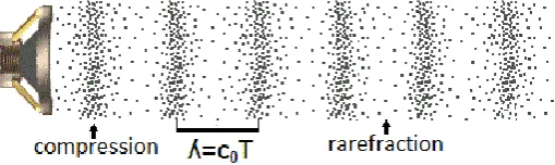
[image:12.595.79.334.560.636.2]

around 343 m/s. In a fluid the velocity of sound is higher. A sound can be produced by a loudspeaker, if the cone of the speaker oscillates it will compress and rarefied the medium. This will increase and decrease the density immediately in front of the cone. The signal is transmitted through space with the speed of sound. The black dots in Figure 4 represent the air molecules. They are compressed and rarefied in a pattern equal to the output signal of the loudspeaker.

Figure 4 Sound waves.

The distance between two compressions, the wave length ʎ, is equal to one period of the transmitted signal multiplied by the speed of sound.

(13)

10

source. Because these changes are so small compared to the ambient value, pressure and density can be considered linearly related. They are related by the following equation:

( 2 )

where p is the pressure [Pa], ρ is the density [kg/m3] and c0 is the speed of sound [m/s]. The particle

velocity is also linearly related to the pressure:

( 3 )

In this equation u is the particle velocity and ρ0 is the ambient density. The product is known as

the characteristic acoustic impedance of the medium.

All fluctuations are very small compared to their ambient values and thus linearly related. Therefore, the principle of superposition may be applied to multiple waves which travel through the same medium.

2.2 Acoustic quantities

The variables pressure and particle velocity determine the acoustic power of a wave. In this section all the power quantities used in this report are introduced.

2.2.1 Sound intensity and acoustic power

The sound intensity is defined as the sound power per unit area. The intensity is the product of pressure and particle velocity:

⃗ ⃗⃗ ( 4 )

The particle velocity and sound intensity are vectors, they have a direction and a magnitude. The acoustic power is calculated by integrating the sound intensity over an surface

| |

( 5 )

In free space waves propagate in all directions, every point of a radiating source emits spherical traveling waves in all directions. The acoustic intensity of spherical waves decays by 1/r2, where r is the distance from the source. This decrease in intensity can be considered a consequence of energy conservation for propagating waves. The energy spreads out over the surface of the expanding sphere. The integral of the sound intensity over the surface of each sphere is equal.

2.2.2 Sound pressure level and sound velocity level

The sound pressure level (SPL) is a logarithmic measure of the sound pressure of a sound relative to a standard reference value. It is measured in decibels (dB) above a standard level:

̅̅̅̅̅̅̅

( 6 )

Pref is a reference pressure of 20 µPa.

(14)

11

( 7 )

Uref is the standard reference particle velocity and is equal to 5.0∙10-8 m/s [31].

The reference values of the SPL and SVL are scaled in such a manner that both quantities produce approximately the same dB level:

→

( 8 )

2.3 Sound radiation from structures

In this section some basic properties of a vibrating panel are treated. The purpose of this section is to relate the velocity of a panel with its sound radiation. Therefore the kinetic energy of the panel is determined and structural modes are examined.

2.3.1 Kinetic energy

When a panel is excited by an external source it starts vibrating. A vibrating panel radiates with a set of structural modes. Dependent on the frequency of the external source and the dimensions of the structure some modes of the structure will be excited. Each mode has a unique vibrating pattern; a two-dimensional standing wave. The response of the panel is equal to the summation of all modes. Thus, the steady state velocity distribution of a panel can be written as:

∑

( 9 )

where 𝑛( ) is the amplitude of the m-th mode, and 𝑛( , ) represents the shape of the mode. The

panel vibrates in the direction orthogonal to its surface. For a panel of dimensions Lx by Ly with edges

that can not have any linear motion the structural mode shapes are given by

𝑛 (𝑛 ) 𝑛 (𝑛 ) ( 10 )

where n1 and n2 are the modal integers. The structural mode with n1 = 1 and n2 = 3 is referred to as the

(1,3) mode. In figure xxx the shapes of some of these modes are shown.

(15)

12

The total kinetic energy of the panel is equal to the total mass multiplied by the mean-square velocity. Its equation, is shown below

∫ | | ( 11 )

where S is the surface area of the panel. The mean squared surface integral of the shape of a structural mode has the property that it is equal to one

∫ ( 12 )

Thus by combing equation ( 9 ) and ( 11 ), the kinetic energy can also be written as a summation of the amplitudes of the structural modes times the mass of the panel

∑| |

( 13 )

Each structural mode has a self radiation efficiency, this efficiency relates the amplitude of the structural mode with the radiated power. The efficiency of a structural mode is determined by its shape and by the excitation frequency. Especially structural modes that have a net volumetric component are efficient. These are the modes that have an odd modal integer, for example, the (1,3) mode. Modes with an even modal integer radiate much less efficient, for these modes the air in front of the panel can transfer from one side of the panel to the other, which will not result in a sound field.

2.3.2 Radiated sound power

The sound fields of different structural modes interact. If the panel vibrates with two modes there is a mutual radiation efficiency. Besides the original self radiation efficiency, an extra component is radiated. The radiated sound power is related by the amplitudes of the structural modes by the following equation

( 14 )

where a is the vector of all mode amplitudes and matrix M contains all radiation efficiencies. The diagonal terms are the self radiation efficiencies and the off-diagonal terms are the mutual radiation efficiencies.

If the panel is lightly damped and excited close to the resonance frequency of the m-th mode, then only this structural mode will contribute significant to the kinetic energy of the panel. Excitation in the region between resonance frequencies will excite all modes a little. At these frequencies almost no reduction in radiation power is possible.

Excitation frequencies with wavelength smaller than the dimensions of the panel will excite multiple modes of the panel. Thus, for low frequencies the far-field sound radiation of a plate is proportional to the kinetic energy of the panel.

2.3.3 Controlling a radiating panel

(16)

13

from their output. However, in most applications the kinetic energy is estimated by using equation

( 11 ).

In theory, with structural actuators the velocity of the structure can be cancelled. In this situation the panel has no kinetic energy, thus no sound is radiated. In practise, however, the vibration can often only be reduced by the action of secondary actuators, and minimising the total kinetic energy of a structure does not generally result in the minimisation of radiated sound. In fact a reduction of vibration may be accomplished by an increase in sound radiation.

3 Adaptive Harmonic Decentralized Feedforward Controller

This chapter starts with a basic harmonic feedforward control algorithm, each section this algorithm is extended till a decentralized adaptive harmonic feedforward controller is obtained. The stability and convergence rate of the controllers is analysed. Control effort weighting is added to the algorithms to stabilize them. In the principle component space the effect of effort weighting is examined. The last sections of this chapter focus on the detection of the harmonic error signals.

3.1 Harmonic feedforward controller

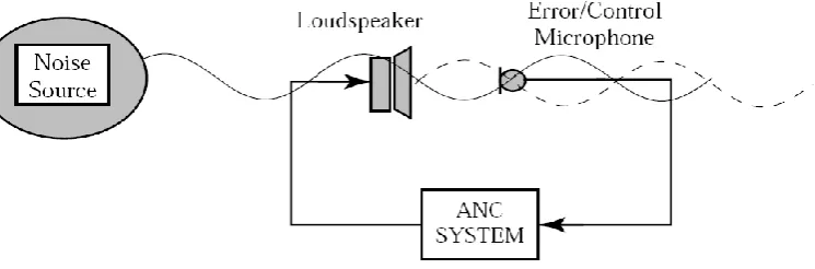
[image:16.595.84.457.398.521.2]

In Figure 6 the most basic active noise control system is shown. An external source produces a single tone deterministic disturbance signal d(n). This disturbance signal is measured by microphone, which is connected to the active noise control system. The measured signal is called the error signal, e(n).

Figure 6 The principle of anti-sound.

The controller will try to produce a control signal, u(n), that will completely cancel the disturbance signal at the microphone. The active noise control system will succeed in this task if it knows the complex transfer function between the loudspeaker and microphone. This transfer function, G, is called the complex frequency response of the plant. The error signal can thus be written as follows

𝑛 𝑛 𝑛 ( 15 )

The disturbance signals of the propeller engines contain multiple tones. And beside these tones background noise is present in the measured signal. However, a controller very similar to the above mentioned method can be created in the frequency domain. The sampled periodic disturbance signal of the propeller engines can be represented as a finite summation of its harmonics

𝑛 ∑

(17)

14

where k is the harmonic number, Dk is the complex amplitude of the k-th harmonic.

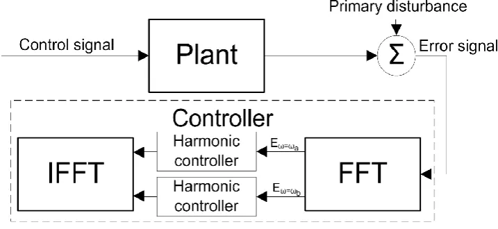
[image:17.595.71.430.169.334.2]

The control algorithm can be divided in K independent loops, each operating on an individual harmonic. Our application only needs to control a couple of harmonics. All other harmonics are not processed. In Figure 7, a harmonic controller in the frequency domain is shown.

Figure 7 An implementation of the frequency-domain harmonic controller.

This controller uses a Fast Fourier Transformation to transform the error signal to the frequency domain. Then a couple of harmonics are selected which are processed independently. The resulting control signals are joined and transformed back to the time domain. The error of the k-th harmonic can be written as

( ₎ _{( 17 )}

The optimal control signal for this harmonic is:

( 18 )

(18)

[image:18.595.69.371.67.212.2]

15

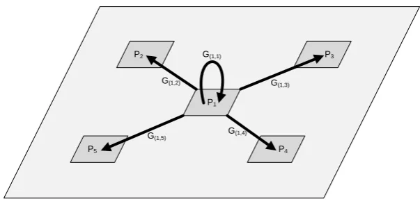
Figure 8 Mulitchannel plant response.

Also the disturbance signal has a transfer function to all error sensors. For a multichannel system equation ( 17 ) is extended to a vector form

( ₎ _{( 19 )}

where G is a matrix of the complex plant responses. All other elements are vectors.

Not in all applications it is possible to produce control signals equal to its optimal value. For example, the control signals might be limited to an upper bound. As a result not all disturbance signals are cancelled at the error sensors. The problem of finding the optimal value for the control signals can be split into L independent optimisation problems. However, most of the time a general formulation is used which weights all error signals equal. Its cost function is defined as the sum of the square error signals

𝑛 𝑛 𝑛 ( 20 )

3.2 Adaptive harmonic feedforward controller

The harmonic feedforward controller presented in the previous section works only under perfect circumstances. In practise, due to environmental changes the responses might change over time. Temperature changes for example, change the speed of sound (see section 2.1 ) which will change the phase of the received signals. Instead of cancelling the disturbance signal it might now be amplified. Also small measurement errors of the re

Therefore, in this section an iterative algorithm for adjusting the control signals is presented, the steepest descent algorithm. This algorithm updates the control signals at each iteration in proportion with the negative gradient of the cost function with respect to these control variables. This way, the algorithm will converge to the optimal solution. The steepest descent algorithm is shown below

𝑛 𝑛

𝑛 ( 21 )

where J is the cost function, n is the iteration index, and is the convergence factor. The derivative of the cost function is called the complex gradient vector, and can be written as

𝑛

𝑛 𝑛 ( 22)

Combining equations ( 21 ) and ( 22) results in the following algorithm

G(1,1)

G(1,4)

G(1,2) G(1,3)

G(1,5)

P1

P2 P3

P4

(19)

16

𝑛 𝑛 𝑛 ( 23 )

in which is the convergence coefficient

By combing equation ( 23 ) and ( 19 ) the following equation for the control signal is obtained

𝑛 𝑛 [ 𝑛 𝑛 ] ( 24 )

This equation will reach a steady-state solution when U(n+1) is equal to U(n). The term in the square brackets is zero under these circumstances. The optimal control signal is thus equal to:

( 25 )

This is equal to the optimal solution of the non-adaptive feedforward controller.

The drawback of an adaptive controller is that the algorithm only converges to its optimal solution if a number of conditions are met. In an unstable system a certain parameter of the system cannot be controlled from the outside. This will result in an uncontrollable output signal, which can reach an unlimited value. The input signal will not be able to influence this output.

The convergence of the algorithm can be examined by combining equation ( 24 ) and ( 25 )

𝑛 ( 𝑛 ) ( 26 )

Equation ( 26 ) can be rewritten to the following form, assuming U(0)=0

𝑛 ( 27 )

The control signal can only obtain its optimal value if equation ( 27 ) converges. The convergence of this equation is determined by the eigenvalues of the matrix GHG. This matrix is called the Hessian matrix, and it is the second derivative of the cost function with respect to the control signal. The real parts of all the eigenvalues must be positive for the equation to converge.

Furthermore, there is a limit on the convergence coefficient . The steepest descent algorithm will only converge if

| | ( 28 )

The above equation will be proven in the principal component space in section 3.6. For complex eigenvalues this equation can be written as

| | ( 29 )

3.3 Control effort weighting

(20)

17

An unstable system can become stable by the addition of a control effort weighting factor in the control law. The cost function for this system is defined as follows

𝑛 𝑛 𝑛 𝑛 𝑛 ( 30 )

This cost function will not minimise the squared error signals, but a combination of the squared error signal and the squared control signals. So the optimal solution of this cost function will not cancel all disturbance signals. The derivate of the cost function, the complex gradient vector, is shown below

𝑛 𝑛

𝑛 𝑛 𝑛 ( 31 )

The steepest descent algorithm with control effort weighting is shown in the equation below

𝑛 𝑛 𝑛 𝑛 ( 32 )

By following the same steps as in the previous section the optimal control signal of this algorithm is derived

[

]

( 33 )

And the convergence of the algorithm depends on, assuming that U(0)=0

𝑛 [ ] ( 34 )

The addition of the control effort weighting factor changes the eigenvalues of the system to the following values

( 35 )

Thus by adding a control effort weighting factor an unstable system with negative eigenvalues can be made stable. Hence, the minimum required control effort weighting is

( 36 )

The convergence criteria presented in the previous section is still valid for this system, however the new eigenvalues should be used in the equation. In section 3.6.2 the effect of effort weighting on the average squared error will be demonstrated.

3.4 Decentralized controller

In this section decentralized control and the effect of plant uncertainties are introduced. From the theory of the latter the effect of decentralized control can be derived.

3.4.1 Effect of plant uncertainties

(21)

18

behaviour of the adaptive algorithm, the system might become unstable and a different finale state may be reached. The steepest descent algorithm with effort weighting and plant uncertainty is shown below

𝑛 𝑛 ̂ 𝑛 ( 37 )

The addition of plant uncertainty to the steepest descent algorithm changes the optimal steady state control effort to

[ ̂ ]

_̂

( 38 )

3.4.2 Decentralized controller

From the model of uncertainty in the plant response estimation a decentralized control algorithm can be derived. If the elements of the plant response matrix G are known or can be reliably measured, ̂ can be set equal to the diagonal elements of G. Hence, each control signal is only updated by one error signal. This means that there are now k independent controllers, with an actuator sensor pair and they only know the response function between these two elements. For a system with three actuator sensor pairs the estimated plant response is thus given by

̂ [

] ( 39 )

When and ̂ are known the stability of the system can be calculated. The same rules for stability apply for a decentralized system as for a centralized system, the eigenvalues of the matrix (̂HG+βI) must be positive. Else will the adaptive algorithm given in equation ( 34 ) will not converge. Because the decentralized plant response estimation matrix ̂ contains only diagonal elements, the system will be more unstable and require larger effort weighting to become stable.

3.5 Gersgorin’s Theorem

With Gersorin’s theorem the location of the eigenvalues are estimated. This technique might be useful for decentralized application. Because it does not require knowledge of the complete complex frequency response matrix at each decentralized location. In this section this method is

demonstrated.

3.5.1 The theorem

In the equation below a square matrix A is given:

[

] ( 40 )

Every eigenvalue of this matrix satisfies at least one of the inequalities:

| | ∑| |

(22)

19

Thus, each row of matrix A gives information on the location of a single eigenvalue. This eigenvalue will lie inside a circle region which is centred at aii and has a radius equal to the sum of all other

elements of that row.

If a square matrix is transposed, then its eigenvalues do not change. Thus, equation( 41 )is also valid for the columns:

| | ∑| |

( 42 )

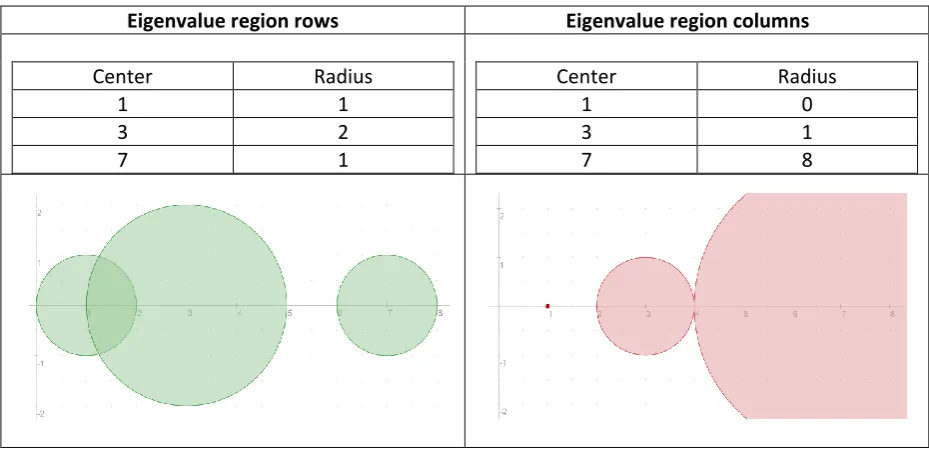
By combining these two methods an even better assumption of the eigenvalues can be made. Let’s illustrate this theorem with a small example. For the square matrix A the following values are chosen:

[

]

The diagonal elements of this matrix are the centres of the circles, in which the eigenvalues must lay. The sum of the non-diagonal elements in the associated row or column determines the radius of the circle. This is shown in Figure 9.

Eigenvalue region rows Eigenvalue region columns

Center Radius

1 1

3 2

7 1

Center Radius

1 0

3 1

[image:22.595.65.530.387.613.2]

7 8

Figure 9 Eigenvalue regions

(23)

20

Figure 10 Combined eigenvalue regions

The estimation of the region in which the eigenvalues must lie can be further improved by applying a similarity transformation. There are however, an unlimited amount of similarity transformations possible which all can be combined whit each other.

An equivalent matrix of A can be created by applying the similarity transformation TAT-1. This transformation creates a matrix which has the same eigenvalues as the original matrix A.

_[ _{] [}

] [

]

[

_]

( 43 )

From this result the following equation is derived, every eigenvalue of this matrix satisfies at least one of the inequalities:

| | ∑ | |

( 44 )

3.5.2 Gersgorin’s theorem and decentralized control

With Gersgorin’s theorem each decentralized controller can calculate its own control effort weighting factor. For this calculation it only requires the complex transfer functions from all actuators to its own sensor.

The convergence of the adaptive decentralized feedforward algorithm with effort weighting is determined by the eigenvalues of the matrix ̂ . Applying Gersgorin’s theorem on this matrix will result in a stability matrix A, which has the diagonal elements:

| | ( 45 )

which are real and positive, the off-diagonal elements being

(24)

21

By using equations ( 45 ),( 46 ) and( 41 ) the following law can be derived, which guarantees stability

| | ∑| |

_{( 47 )}

This equation can be rewritten in the following form

| | | |

⁄ ∑| |

( 48 )

As explained earlier in this section a region is calculated in which the eigenvalues may lie. Thus, Equation ( 48 ) provides a sufficient condition for the stability of a decoupled system, but not a necessary one. It is possible that equation ( 48 ) is not satisfied and yet the system is stable.

3.6 Principal component analysis

In this section the complex plant response will be transformed to its principal components. This will result in a new block diagram and a new formulation of the cost function. The principal component form provides more insight in the behaviour of the system. With this information the effect of effort weighting is demonstrated. Also the algorithm will be investigated, to show if it can be used in a decentralized control system.

3.6.1 The algorithm

In a multichannel control system, different modes are excited by the disturbance signal. By transforming the complex plant response to its principal components the contribution to the error signal of each individual component can be determined. Each component has its own power and its own convergence rate.

The singular value decomposition of the complex plant response of a system with L error sensors and M actuators is defined as

( 49 )

The unitary matrix R contains the complex eigenvectors of GGH and the unitary matrix Q contains the complex eigenvectors of GHG. The L columns of R and the M columns of Q are called the left singular values and the right singular values, respectively. Ʃ represent the singular values matrix, this is an L by M matrix, the diagonal components contain the singular values all other elements are equal to zero. The singular values,

,

are sorted by size; the upper left element of the matrix contains the largest singular value. The singular values are equal to the square roots of the eigenvalues,

,

of the matrix GHG or GGH

√

( 50 )

(25)

22

( 51 )

Using equations ( 30 ),( 33 ),( 51 ) and ( 52 ) the optimal control signal without control effort weighting is now given by

[

]

( 52 )

By combining equation ( 15 ) and ( 49 ) and multiplying both sides by RH the following equation is obtained

𝑛 𝑛 ( 53 )

This equation can be transformed to a useful form which is given by

𝑛 𝑛 ( 54 )

In this equation a few new terms are defined; the transformed input signal y(n), the transformed disturbance signal p and the transformed control vector v(n):

𝑛 ( 55 )

[ ] ( 56 )

𝑛 𝑛 ( 57 )

In Figure 11 the block diagram of this transformed system is shown. Because only the diagonal elements of the matrix ∑ contain a value that is non-zero, every transformed error signal y is only a function of a single transformed disturbance function and a single transformed control signal (when the number of sensors and actuators is equal).

Figure 11 Principal component block diagram of a multichannel tonal control system.

By minimalizing all the independent components of y(n) the error signal e(n) is minimalized as well . Thus the optimal values for the individual transformed control signals are:

( 58 )

Because the matrix R is unitary the cost function can be written as a function of y(n)

∑ | |

(26)

23

The behaviour of a system which is transformed to its principal components is not changed. So the convergence behaviour is still the same. The benefit of this transformation is that the individual components of the error signal are better observable and controllable. With this transformation it is possible to only control the principle components that contribute most to the error signal. The other principal components will just be ignored, and so not proportional high control signals can be avoided.

The adaptive feedforward algorithm of equation ( 23 ) is written in the principal component form as follows:

𝑛 𝑛 𝑛 ( 60 )

Because ∑ is a matrix with only diagonal elements the above equation van be written as M independent equations:

𝑛 𝑛 𝑛 ( 61 )

By combing equations ( 61 ),( 58 ) and ( 54 ) and using the fact that the following equation is obtained

( 𝑛 ) ( ) ( 62 )

The limitation on the convergence coefficient as shown in section 3.2 is proven by the above equation.

The convergence behaviour of the cost function is shown below. Every mode converges

independently. Of course only the modes which are controlled will converge, the modes that are not controlled will always contribute | | to the cost the function.

𝑛 ∑ | |

( 63 )

3.6.2 Effort weighting

As explained in section 3.2 only modes with a positive eigenvalue will converge (see for example equation ( 63 ) ). Systems with negative eigenvalues are unstable and must be made stable by adding effort weighting. In the principal component form effort weighting is added as follows:

[

]

( 64 )

The optimal control signal is obtained by a similar derivation as in the previous section

[ ] ( 65 )

(27)

24

∑

|

( 66 )

3.6.3 Conclusion

The principal component form gives a good overview of the effect of effort weighting. Modes for which will not have their contribution to the sum of the squared errors removed by the control algorithm. A suitably chosen value of will not only make the system stable, but can also prevent physically unreasonable values of control effort.

Some applications only control the modes that contribute most to the total error. A decentralized implementation of such a system is not possible. Modes are not related to sensor actuator pairs. A system that controls only a couple of modes requires the information of all sensors, and has to control all actuators. This information can only be processed by a centralized controller.

3.7 Phasor arithmetic

In a harmonic controller all calculations are performed with phasors. A phasor is a representation of a sine wave whose amplitude and angular frequency are time-invariant. Phasors decompose the behaviour of a sinusoid into two components; amplitude and phase.

The sensors of the system measure a continuous time error signal, which is assumed to have a constant frequency and amplitude, this signal is transformed to a phasor. Then some calculations are performed, which will result in a control signal in phasor form. This phasor is transformed back to a continuous time signal and transmitted by the actuator. In this section the best methods for these phasor operations are examined.

All sinusoid signals have a phase and amplitude. In the equation below, a cosine is written as a complex signal:

{ _} _{( 67 )}

In this equation is the phasor. A phasor can be stored with an amplitude and phase component or with a real and imaginary component.

Two complex numbers are multiplied as follows (using real and imaginary components):

( 68 )

This equation can be modified to a form that uses only three distinct multiplications to calculate the real and imaginary part [32]. This new formulation requires a few extra additions, however on most systems the computational cost of additions is much less than multiplications.

[ ] [ ] ( 69 )

The process of multiplying two complex numbers is best visualised in polar coordinates. The complex signal can be converted to a magnitude and phase signal.

[

𝑛

]

( 70 )

(28)

25

[ 𝑛 ] ( 71 )

In polar coordinates only two operations are required, the magnitudes of the two signals are multiplied and the two phases are added to each other. However, addition is much harder in polar coordinates. For an addition operation the signals need to be transformed to complex numbers before they can be added. This is shown in the equation below:

( ) ( 𝑛 𝑛 ) ( 72 )

𝑛 ( 𝑛 𝑛

) ( 73 )

3.8 Error signal detection

The error signal produced by a rotating propeller consists only of a few frequency components. Its main error component is equal to the blade passage frequency. The other excited frequencies are higher harmonics of this fundamental frequency. The harmonic controller only has to know the errors of these frequencies. In other frequencies the controller is not interested. In this section, three techniques are presented for the detection of the phase and the magnitude of these error

components. In the final part of this section, these techniques are compared and the best solution is chosen.

3.8.1 Fast Fourier Transformation (FFT)

A Fast Fourier transformation (FFT) measurement of the spectrum has two possible sources of errors. The first one is the aliasing error, the power of higher frequencies is mirrored at the lower

frequencies. This can be avoided by setting the sample frequency higher than 2 times the highest frequency present in the measurement signal. Generally it is advised to low pass filter the

measurement signal before applying a FFT operation. The second source of error is called the leakage error, single frequencies will be smeared out in neighbouring frequency bins. This error appears if no integer number of periods of the excitation signal is measured. This problem can be avoided by changing the configurations of the measurement setup, for example by adjusting the duration or the sample time of your system. If this is not possible the error can be minimized by using a window other than a rectangular window. In general, a window will smoothly weight the first and last samples of a measurement less heavy in order to decrease the discontinuities of the measurement signal.

The spectrum is split in different frequency bins. This introduces another limitation, the desired signal must be exactly centred in a frequency bin. Else its power is spread into the two closest bins.

The FFT algorithm has to gather all N samples before it can calculate the spectrum. Thus, it has to store all these samples temporarily.

3.8.2 Goertzel algorithm

The Goertzel algorithm identifies only a single predefined frequency component of a signal. While an FFT analyses the entire spectrum. Multiple implementations of this algorithm are required to

measure multiple frequency components. The Goertzel algorithm computes the following sequence:

(29)

26

where (s-2) and s(-1) are equal to zero. From this sequence the phasor of the signal can be derived with the following equation

_{𝑛 𝑛} _{( 75 )}

A great advantage of this algorithm compared to the FFT is that there is no leakage error. Thus an arbitrary length of the measurement can be chosen. This reduces the complexity of the measurement setup. Also the algorithm can process samples as they arrive. Only when all samples are received a small extra operation is required to calculate the phasor.

The frequency resolution of the Goertzel algorithm is the same as for the FFT. Thus, the same number of samples is required to remove the effect of undesired neighbouring frequency components.

3.8.3 Linear Least Square (LLS) technique for phase estimation

The LLS phase estimation technique uses a maximum likelihood (ML) approach for an optimum estimation of the phase and amplitude of the signal. This method can find multiple frequency components with a single operation.

A signal that consists of M sinusoids can be written as follows:

𝑛 ∑ 𝑛

( 76 )

where Am>0, ωm ϵ (0,π) and φm ϵ (-π,π) denote the amplitude, frequency and phase of the m-th

sinusoid. The cosine term of a single sinusoid can be written as the product of two vectors:

𝑛 [ 𝑛 𝑛 ] [ _] ( 77 )

Notice that the second vector is not dependent on n, and contains all phase and amplitude information of the signal.

Each measurement N samples are measured. And from these samples the phase and amplitude are derived. Equation ( 77 ), can be rewritten as a vector of N samples:

( 78 )

where [ ] , α is a 2 by 1 vector and H is a N by 2 matrix. In this equation H is a reference signal with which the input signal is compared. The phase and amplitude differences are stored in α. The reference signal H has the following format:

[

𝑛

𝑛 ]

(30)

27

where A1 and are the reference amplitude and phase. Thus, to find the phase and amplitude of the input signal x, parameter α must be estimated. The LLS estimate for α is computed as:

̂ _{( 80 )}

The LLS method calculates (HTH)-1 for each measurement. If the reference signal is the same for each measurement this has to be done only once. By extending the vectors multiple signal components can be detected (see So [33]). The detection of multiple frequency components will increase the size of the matrix HTH, this will significantly increase the complexity of the inverse operation performed on this matrix.

The accuracy of this method is equal to the Goertzel algorithm. If these two algorithms are tuned to detect only a single frequency component their frequency responses are exactly the same.

3.8.4 Comparison

The disturbance measured by the sensors can obtain any frequency within a certain range, and this frequency may change over time. The FFT method is not flexible enough for this situation. It can not centre a frequency component in a frequency bin for all situations. This will introduce unacceptable large errors in the estimation. Therefore, only the Goertzel algorithm and the LLS phasor estimation method can be used for this application.

In the table below the computational complexity of the different algorithms are shown. Unlike all other methods the LLS method compares its phase to a reference phase. Therefore, this method is considerably less efficient. In this table also the simple DFT method for a single frequency bin is shown.

Multiplications Additions / subtractions Sinusoid function

computations

Radix-2 FFT 2N log2(N) 3N log2(N) 2N

DFT single frequency bin

2N 2N 2N

Goertzel algorithm N+2 2N+1 2

LLS phasor estimator (3+2)N (3+2)N 2N

In the harmonic controller first the LLS phasor estimator technique will be implemented. This method is chosen because it has the best accuracy and is easy to implement. Later this method will be

replaced by the Goertzel algorithm because it is less computational complex and has the same performance.

4 System identification

(31)

28

In this chapter various system identification techniques are presented. These techniques are compared and the best solution is chosen. The important factors in this decision are measurement time and system complexity.

4.1 Possible implementations

The dynamic behaviour of a system can be derived from measurements of the input and output signals. In the double-panel structure it is possible to excite each input with an arbitrary chosen signal. In normal operating mode the decentralized actuator sensor pairs do not need to

communicate with each other. Thus, no centralized controller is required. However, in the system identification phase communication between these elements is required, there has to be a

mechanism that tells each decentralized controller when it has to listen and when it has to produce a control signal. Else, all components will talk at the same time and no information of the system is obtained. Of course, the best option is to limit the communication between the elements as much as possible. The disadvantage of such systems is that each controller has to calculate complex functions, for which complex hardware is required. This hardware might not be needed in normal operating mode. However, there are also techniques that require less complex hardware but they might be too slow.

The system identification process can be performed with the following three configurations

Decentralized System identification

The first implementation is almost completely decentralized. One after the other, all actuators will produce an excitation signal. During this stage all sensors will listen to the response. This way, all decentralized controllers will know the response from all actuators to their sensor. According to Gersgorin’s theorem this is enough for a stable system. With this information they can calculate their own values for alfa and beta

Decentralized data analysis, centralized parameter calculation

This implementation uses the same techniques to determine the transfer functions as the first method. Now, however the calculated transfer functions are sent to a centralized controller which will determine optimal values for alfa and beta.

Centralized system identification

All data received by the sensors is directly sent to a centralized controller which will calculate the transfer functions between all elements. This centralized controller will then configure each decentralized controller

4.2 Excitation signals

(32)

29

frequency, refined waveforms with a broadband spectrum are generated. These waveforms collect all spectral information in just a single measurement.

4.2.1 Measurement time

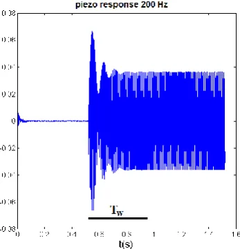
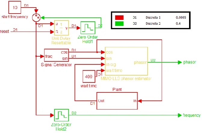
[image:32.595.71.245.276.457.2]

Before the transfer function of the system can be measured, the system has to reach its steady state. Every time the source signal changes it takes some time before the response is stable and periodic again. This initial situation is often called the transient state or the warm-up period. In the transient state the response changes due to the different time delays of the transmission paths between the actuators and the sensors. Remember that there are multiple transmission paths between a single actuator and sensor (due to reflections in the system). In Figure 12, this situation is shown for the actual system. At t=0.5s a single actuator is turned on, producing a 200 Hz signal. After a waiting time TW the response is approximately stable. This waiting time is approximately 0.4 seconds; it is the same for all excitation frequencies.

Figure 12 Wait time of the double-panel structure.

The stepped sine method has to wait Tw seconds at each frequency before it can measure the

response. For an accurate measurement only a few samples are required when for example a Goertzel algorithm is used (this algorithm does not need a complete period of a sine for accurate results). The measurement time of the stepped sine method can thus be expressed as:

( 81 )

where Tm and F denote the measurement time of a single sinusoid and the number of frequency

steps.

A broadband excitation contains a single period in which all frequencies in a specified range are excited. This period is repeated so that a periodic signal is created. When there is a good SNR this method only has to measure a single period. This measurement contains information for all

frequencies. This measurement can start after the transients have disappeared, thus after a waiting time Tw. The broadband measurement time is

(33)

30

where is the frequency resolution, one period of the broadband measurement equals 1/ .

A broadband signal distributes its power over F frequencies, while a stepped sine measurement concentrates all its power on a single frequency. Thus, the SNR ratio is much higher for the stepped sine method. To compensate for this poor SNR often the average of multiple periods of broadband excitation is used.

4.2.2 Broadband excitation signals

In this section broadband excitation signals are examined. The goal of this section is to understand the basics of these methods and to determine which resources are required to generate them and what is needed to extract information from their response. Broadband excitation signals are

discussed in more detail by Pintelon [34]. In this section, two deterministic signals are inspected and a general conclusion about random excitation signals is presented.

Periodic chirp

This is the most basic broadband excitation signal. In one period a sine is swept from its lowest to its highest frequency. This is repeated so that a periodic signal is created.

𝑛( ) ( 83 )

With T0 the period, , , . The lowest frequency in this equation

is and the highest .

A periodic chirp can be generated by a single frequency controlled oscillator. This component is already present in the original setup. From the response all frequency components must be extracted by a FFT operation.

Schroeder multisine

The Schroeder divides it power in all frequencies equal. This broadband excitation signals is created by adding all frequency component together. This is shown in the equation below

∑

( 84 )

with Schroeder phase .

(34)

31

Figure 13 Broadband excitation signals in the frequency domain.

The main problem of the Schroeder multisine method is that it requires a FFT technique to generate the signal. This is too complex to implement it decentralized. For the analysis of the response also a FFT operation is required.

Random excitations

The mayor difference compared with periodic excitations is the variation in excitation from one realisation to the other. A random signal is transmitted by the actuator and received by the sensor. To extract the frequency response the original signal is required. This means that this method cannot be implemented decentralized. The original signal is only known at its source.

Deterministic excitations also have superior properties compared with random excitations. Random excitations putt less power in the system and are prone to leakage errors.

4.3 Conclusion

The preferred method for system identification is the decentralized implementation. In experiments the performance of such a system must be compared with a system which calculates the control effort weighting factor and the convergence rate centralized (see section 3.2 ). If the performance degration of the decentralized controller under normal circumstances is not very huge this method will be used. Else one of the other two methods should be chosen. Decentralized data processing might reduce the requirements on the data transport between the decentralized controllers and the centralized controller. Therefor as an alternative this method is chosen.

The extra hardware required for analysing and producing the excitation signals must be as little as possible. Hence, the best method is the simple stepped sine excitation signal. All hardware for this method is already present on the decentralized controllers. To accelerate this process a few frequencies can be analysed in parallel, similar to the Schroeder multisine method

5 Simulations

(35)

32

This chapter contains two sections. In the first section the control effort weighting factor for a decentralized controller is calculated for the entire frequency range. The resulting effort weighting factor will show if a decentralized implementation in the double-panel structure is realisable. In the second section a decentralized feedforward control system is created. This system will also contain a model of the plant, so that the performance of the controller can be analysed.

5.1 Control effort weighting

In this simulation the minimum control effort weighting factor β for the experimental setup is determined for the entire frequency range. In Chapter 3, two methods were presented to calculate the control effort weighting factor. The first method is an optimal solution based on the eigenvalues of the Hessian matrix of the cost function (see section 3.3). The second method uses Gersgorin’s theorem (see section 3.5). This method is not optimal but easier to implement in a decentralized application.

The main goal of this section, is to determine if noise reduction can be realized by decentralized control of the double-panel structure. With equation ( 66 ) from section 3.6.2, shown below, this is analysed.

∑

|

If the system has a mode with an eigenvalue that in size is comparable to the effort weighting factor, then for this mode attenuation of the disturbance can be achieved. Therefore, in this analysis the largest eigenvalue is compared with the effort weighting factor.

Below, equation ( 47 ) from section 3.5.2 is shown. With this equation the effort weighting factor is determined according to Gersgorin’s theorem.

| | ∑| |

The ratio of | | to is determines if Gersgorin’s theorem can make an accurate estimate of the eigenvalue. If beta is much larger than the square of the direct coupling than this theorem is not very useful.

First a configuration which only controls the radiant panel is examined. Then a system using both panels is analyzed and as last the effect of feedback is shown.

Controlling the radiant panel

With the data from the finite element model the values for , , | | and

(36)

33

Figure 14 Simulation results of actuator sensor pair 1.

The beta determined by the eigenvalues of the Hessian matrix is lower for most frequencies than the beta of Gersgorin’s method. However for some frequencies with Gersgorin’s method a lower value for beta is obtained, this is because Gersgorin’s method calculates for each decentralized controller a separate value for beta. A lower beta at a single decentralized controller will result in higher values for beta at the other decentralized controllers. Hence, the overall performance of the eigenvalue method is better. In Figure 15, the simulation results for another decentralizd controller are shown, to demonstrate this effect. For frequencies between 300 and 400 Hz the effort weighting factor is now higher for Gersgorin’s method.

Figure 15 Simulation results of actuator sensor pair 2.

(37)

34

Figure 16 Actuator sensor pair 1: Direct coupling versus cross coupling.

Controlling both panels

If the decentralized controllers of both panels are used there is more cross coupling. Each sensor receives a signal from all sources. Which makes the overall contribution of the own actuator smaller. In Figure 17, the normalised received power of the centre sensor of the radiant panel is shown. At low frequencies the cross-coupling between the two panels is significant. At higher frequencies only the actuator in the middle of the incident panel has a significant contribution to the cross-coupling.

Figure 17 Actuator sensor pair 1: Direct coupling versus cross coupling both panels.

Controlling the radiant panel with feedback

In Figure 18 beta is determined for the decentralized control in the middle of the radiant panel with feedback. The feedback reduces the direct coupling, the values of| | are smaller. For large regions the ratio (eigenvalue) to max eigenvalue is smaller with feedback. However, there are some

Active noise reduction in double panel structures : decentralized adaptive feedforward control

MASTER THESIS