Faculty of Electrical Engineering, Mathematics and Computer Science (EEMCS)
Constructing
an
α
-maximizing
option trading strategy in a
multi-dimensional setting
Peter Bosschaart (s0176761)
Assessment Committee: Prof. Dr. A. Bagchi (UT/SST) Prof. Dr. P. Guasoni (DCU/Stokes) Dr. Ir. E.A. van Doorn (UT/HS) Dr. B. Roorda (UT/IEBIS) Supervisors:
Dear reader,
Thank you for taking interest in this thesis, which I have written as final project for my Master’s in Applied Mathematics at the University of Twente. The research for this thesis was conducted at the mathematics department of the Dublin City University, Ireland, under the primary supervision of Professor P. Guasoni. I would like to use this moment to express my gratitude to the people who have supported me throughout this project.
First of all, I would like to thank Professor P. Guasoni for giving me the opportunity of working with him and inviting me at the Dublin City University, giving me the chance to go abroad for my studies. It was a pleasure to work with him and I really appreciate the way in which he has supervised me. I am grateful for the informal, but professional atmosphere he provided and the way he always could find the time to meet with me to discuss the project.
Second, I want to thank Professor A. Bagchi for supervising me at the University of Twente, especially in the last phase of the project. I wish him all the best in his retirement.
Third, the people of the mathematics department of the Dublin City University, for welcom-ing me in Ireland and at the Dublin City University. It was a pleasure to work alongside this group. I would especially like to thank Dipl.-Ing. Dr. Eberhard Mayerhofer, who I came to know as a good friend, and who took the time to read the concept version of this thesis and provided me with a lot of useful feedback to establish the final version. Also, I would like to thank Christopher Belak, MSc. for being a good friend and introducing me to the city Dublin, as well as for setting up the database structure for the Optionmetrics database and teaching me the basics of MySQL language.
Finally, I would like to thank all other people who provided me with feedback on the con-cept version of the thesis, who supported me in academic or in personal ways throughout the project, and all my friends and family who visited me in Dublin during my time there, providing pleasant distractions during the weekends.
Abstract 1
1 Introduction 3
2 Review of previous research 7
3 Performance maximization with a single benchmark asset 13
3.1 Model formulation . . . 13
3.2 The Markowitz portfolio selection procedure . . . 16
3.2.1 Explicit expressions for the expected excess returns and covariance of excess returns of options . . . 19
3.2.2 Hedging . . . 21
3.3 Model extensions . . . 24
3.3.1 A dynamic growth rateµ . . . 24
3.3.2 Trading costs . . . 25
4 Performance maximization with multiple benchmark assets 27 4.1 Markowitz portfolio selection for multiple benchmark assets . . . 27
5 Simulations 33 5.1 Simulations with a single benchmark asset . . . 33
5.1.1 Varying parameters . . . 38
5.2 Simulations with multiple benchmark assets . . . 40
5.2.1 Varying parameters . . . 46
6 Market data and strategy performance analysis 49 6.1 Historical data on the benchmark assets . . . 49
6.2 Strategy performance analysis with a single benchmark asset . . . 53
6.2.1 Methodology . . . 53
6.2.2 Results . . . 54
6.3 Strategy performance analysis with multiple benchmark assets . . . 70
6.3.1 Methodology . . . 70
Bibliography I
A Proofs III
A.1 Proof of Theorem 3.2.3 . . . III A.2 Proof of Theorem 3.2.4 . . . IV A.3 Proof of Theorem 4.1.1 . . . V
B Tables IX
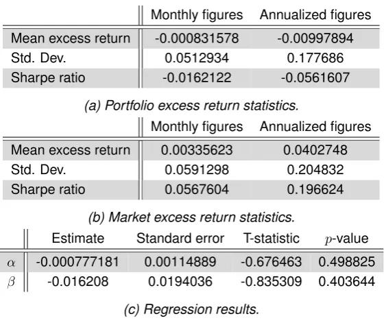
In this thesis we derive a trading strategy which maximizes its excess returns, whilst control-ling for the standard deviation of these excess returns, by dynamically investing in a portfolio of European call options on one or multiple benchmark assets and the benchmarks themselves. We show that this implies that the Sharpe ratio of these excess returns is maximized and that this is equivalent to the maximization of Jensen’s alpha, the intercept in the ordinary least squares regression of these excess returns on the excess returns on the complete US equity market. The strategy is constructed such that the exposure of the obtained excess returns to the excess returns on the complete US equity market is statistically insignificant. The portfolio selection procedure for this strategy turns out to be a variant of Markowitz portfolio selection, adapted to admit derivatives in the selection.
I
NTRODUCTION
A growing literature suggests that a hedge fund manager can generate a positive return on top of the risk free rate (an excess return) by following strategies that repeatedly invest in dynamic portfolios that consist of one or more options on an underlying asset and have the possibility of holding the underlying asset itself. In previous research this has been shown through sim-ulations and examples, but it remains unclear about the magnitude of the excess returns that can be achieved and how big the involved risk is.
Coval and Shumway [1] state that under the Black-Scholes model assumptions, options are redundant assets, but when one deviates from these assumptions, one can generate sig-nificant option returns. Broadie et al. [2] agree and report high returns on-out-of-the money (OTM) puts and straddles on the S&P 500 and explain this by mispricing effects of the market. Eraker [3], Jones [4], Kapadia and Szado [5], Liang et al. [6] and Santa-Clara and Saretto [7] all report similar findings on a variety of underlying assets, however, not all of them control for the involved risk. In these studies the term “risk” is used to denote the standard deviation of achieved excess returns.
This thesis is a follow up research on Guasoni et al. [8], in which a theoretical answer is provided for the questions that are left unanswered by the previous research. In this paper a trading strategy is derived which maximizes the alpha of the achieved excess returns, control-ling for the risk. This paper explains the achieved excess returns by a single factor ordinary least squares (OLS) regression:
rpf =α+βrmkt+ε, (1.1)
where
• rpf is the vector of excess returns generated by the investment strategy,
• α is the regression intercept, which captures the amount of excess return that is gener-ated by the strategy itself (the excess returns linear projection orthogonal to the markets excess return), and is known as Jensen’s alpha,
• β is the sensitivity of the strategy excess returns with respect to the market excess re-turns,
• εis a vector of normally distributed shocks with zero mean, which only add variance to the excess returns.
The derived strategy is a variant of the buy-write strategy, involving long positions in benchmark assets and writing options with a continuous range of strikes on them. For the case where one considers a market that consists of one risky benchmark asset and a safe asset, the authors provide explicit formulae for the weights that one has to invest in each option to achieve the optimal portfolio on every moment on which is traded. The paper concludes from studies with simulated data that if common equity indices are used as benchmarks and if securities on these benchmarks are priced in the Black-Scholes framework, one could generate substantial alpha by trading frequently or holding options. However, such strategies carry a substantial risk as well, resulting in statistically insignificant alphas, and the probability of resulting in a negative alpha is close to one half. Hence, under the Black-Scholes model it is difficult for the hedge fund manager to generate superior performance from trading frequently in derivatives. Nevertheless, when the implied volatility of the derivatives is higher then the realized volatility of the benchmark asset, one is able to produce an alpha in the OLS that is statistically different from zero, even in absence of superior information.
This last conclusion rises the question of whether one is able to produce superior perfor-mance in practice by implementing this strategy on the actual derivatives market, which is the direct motive for the research conducted in this thesis.
In this thesis we formulate the alpha maximizing option trading strategy, which controls for the risk. The strategy repeatedly invests in a portfolio that consists of several options with discrete strikes on an benchmark asset and a position in this underlying asset itself. The selection of the optimal portfolio in this strategy turns out to be a variant of Markowitz portfolio selection theory, which thus far has not been studied very often with selecting derivatives, making it quite a novelty in this thesis. We also hedge out its sensitivity to market movements, to ensure that the generated alpha in regression (1.1) is generated only by our trading strategy. Thus, we want beta in this regression to be a factor of insignificant influence, meaning that its estimate in the OLS regression statistically insignificantly differs from zero at a reasonable significance level. We track the performance of our strategy with the Sharpe ratio, which is defined as the expected excess return generated by the strategy over the standard deviation of its excess returns, hence, a measure of the excess return one can generate per unit of standard deviation. We refer to this standard deviation with the term “risk”. We show that maximizing this Sharpe ratio is equivalent to maximizing the expected excess return given a constant level of variance. We test our strategy in a theoretical setting by simulating data and with historical market data. We use data from the Optionmetrics database, which contains market data from January 1996 to January 2013, to study whether it is possible in theory and in practice to generate a significant alpha under insignificant influence of market movements, and how high the Sharpe ratio that one can generate is.
strategy which repeatedly invests in a range of options that can each depend on a different benchmark asset and in positions in these underlying themselves. We extend our Markowitz portfolio selection procedure for options with discrete strikes to a multidimensional setting, which enables us to test the performance of our strategy with simulated and historical data. In this discrete multidimensional setting we shall again hedge out the sensitivity to market move-ments, to ensure, so to say, “beta-neutrality”. Another novelty of this thesis is that we also study the significance of the other Fama & French factors (the market capitalization factor and the book-to-market factor) in explaining our strategy’s excess returns, by adding them to the re-gression. The main questions are whether one can produce alphas in the OLS regression with this multidimensional trading strategy that statistically significantly differ from zero, whether the strategy’s excess returns are solely generated by the strategy itself, how high the Sharpe ra-tios obtained with this trading strategy can get, and whether the obtained Sharpe rara-tios are higher than those obtained with the one dimensional trading strategy, implying positive effects of diversification.
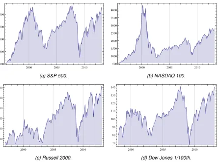
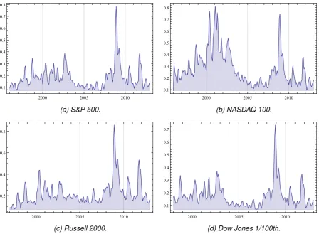
We find that with our investment strategy applied in the Black-Scholes framework it is hard to produce a significant alpha, in the case of a single benchmark asset, as well as in the case of multiple benchmark assets, agreeing with the conclusions in Guasoni et al. [8]. However, we do find that our trading strategy produces a significant, positive alpha and high Sharpe ratios under beta-neutrality when one uses historical market data of the S&P 500, the NASDAQ 100, the Russell 2000, and the Dow Jones 1/100th Industrial Average indices as benchmark assets, during the period of January 1996 - January 2013. The strategy even performs well in times of high volatility on the market (for example the Dot-com bubble period of 1996-2002 and the credit crisis/global recession period of 2007-2013), generating high Sharpe ratios. However, in these times the strategy generates more substantial betas than in periods of low volatility, but which are mostly statistically insignificantly different from zero. Considering more benchmarks to write derivatives on increases the Sharpe ratio of the strategy, thus the effects of diversifica-tion are positive. We also show that our trading strategy in multiple dimensions outperforms a naive multidimensional trading strategy which divides ones wealth equally over all considered underlying and then performs our one dimensional strategy on them. These effects increase when the correlation between the log returns on the underlying increases. We find the other Fama & French factors to be statistically insignificantly different from zero in the regression over the strategy’s excess returns for most of our analyses, which strengthens our claim that the obtained strategy excess returns are generated by the strategy alone, and not by other factors.
R
EVIEW OF PREVIOUS RESEARCH
This thesis is a follow up on Guasoni et al. [8]. In this chapter we introduce and summarize the research presented in the paper “Performance maximization of actively managed funds”, in which the trading strategy is derived that trades in options with continuous strikes on a single benchmark asset and maximizes alpha in the regression (1.1), whilst controlling for the risk. The strategy turns out to be a variant of a buy-write strategy. Since this is a summary, the formulations in this chapter are sometimes very similar to the ones in the paper.
The motivation for the research conducted in this paper is that in previous literature it has been reported that positive regression alphas can be obtained by frequently trading in options, but leaves it unclear what the magnitude of these alphas can be and how big the risk involved is. A theoretical answer to these questions is derived in the paper, providing explicit formulae for the trading strategy that maximizes alpha by trading frequently in options with continuous strikes on a single benchmark, whilst controlling for the risk. In this thesis we bring the theory derived in the paper to practice by formulating the strategy for options with discrete strikes and testing the performance with historical market data. We also extend this strategy such that it can trade in options with discrete strikes that can each depend on a different benchmark.
In practice, an investor who is evaluated by the performance of his fund relative to a bench-mark (for example an index, like the S&P 500 and the NASDAQ 100), can hold this benchbench-mark and write options on it. If the fund is fully invested in the benchmark, the fund return is a lin-ear function of the market return with zero intercept. If the investor writes call options on the benchmark and invests the proceeds in a safe asset, the fund return is a nonlinear function of the market return. If the fund consists of a long position in the benchmark and short position in the options, the fund return has a non-zero alpha in the regression of the fund’s excess return on the excess return of the index. In this framework, the authors pose the optimization problem and its solution.
First, define the excess returnrx on an actively managed fund, which is evaluated against
a vector of excess returnsrm = {r1, . . . , rk}0 on kbenchmark assets. The fund is evaluated
during the period from time0toT, divided in∆t,2∆t, . . . , n∆t, wheren∆t=T, equally spaced time intervals on which returns are observed. Let rxi and rmi denote the observed excess
returns on the fund and the benchmarks respectively, over the time interval from(i−1)∆tto i∆t. The regression over the excess fund returns on the excess benchmark returns is
rxi=α+r0miβ+εi
where the interceptαand the vector of slope coefficientsβ satisfy α=Erx−r0mβ
,
β= (var(rm))−1cov(rm, rx),
and the termεi has zero mean and only adds variance to the excess returns. Then the risk
associated with the benchmark is hedged out by adding a short position ofβ in the benchmark assets, and the return of the hedged position can be expressed asrx−rm0 β, its expectation is
α, and its tracking error ispvar(rx−rm0 β). The appraisal ratio of the hedged position is equal
to the Sharpe ratio:
APR= p α
var(rx−r0mβ)
.
A high appraisal ratio implies high profitability for the hedged position, and as mentioned before, a high T-statistic of alpha in the ordinary least squares (OLS) regression.
The investor wants to maximize the appraisal ratio, so he should find a trading strategy such that the funds returnrxsolves
max
x
E[rx−r0mβ] p
var(rx−r0mβ)
.
One thus has to have a high alpha, but also a low tracking error, to maximize this appraisal ratio.
The space of payoffs available to the investor in a given period by trading in the securities available is denoted with Xa, the attainable space. The payoffs are assumed to have finite
space, and L2(P,Ω) is the set of all measurable functions with finite second moments. The norm on this space is given by ||x|| = E[x2]1/2. The assumption of finite second moments is
a minimal requirement to ensure that the sample estimates of linear regressions converge to their population counterparts. The spaceXaallows the market to be incomplete, because it is
allowed to be a strict subset ofL2(P,Ω). Its dimension could be infinite, which allows options with a continuous range of strikes and maturities on the benchmarks. The only constraint on the linearity of the payoff space.
The linear space of payoffs spanned by the benchmark assets, is denoted by Xb and
re-ferred to as the benchmark space. Its dimension is assumed to bek+ 1. Let{xj}j=0,...,k be the
payoffs of thek+ 1independent assets that span Xb. Let the first payoff, x0, be the constant
payoff of a safe asset. A fund has abnormal return relative to its benchmarks if, and only if, its return or payoff falls outside the benchmark space. This can only be the case ofXb is a strict
subset ofXa.
Letν :Xa 7→ <be the pricing function. Assume that the law of one price holds, thus ν is
linear. Define a stochastic discount factor (SDF) for Xa as a random variable m ∈ L2(P,Ω)
such thatν(x) =E[xm]for allx∈Xa. LetMadenote the set of all SDFs forXawithMa. Then,
by Riesz representation theorem, the exists some ma ∈ Xa such that ν(x) = E[xma] for all
x ∈ Xa, thus,ma ∈ Xa∩Ma. It follows thatma is of smallest norm. The price function also
applies to the set of benchmark assets, so the set of SDFs for Xb is Mb = {m ∈ L2(P,Ω) :
ν(x) =E[mx]for allx∈Xb}, and there exists a smallest norm SDFmb ∈Xb∩Mb.
A trading strategy corresponds to a payoffx∈Xa. Assume that the payoff of the safe asset
isx0 = 1and that its price isν(1)>0. The return on the safe asset is thusR0 = 1/ν(1). One
can then write the excess return on the fund as rx = x−ν(x)R0, and the excess return on
thej-th benchmark asrj =xj −ν(xj)R0 (for i= 1, . . . , k). Let rm ={r1, . . . , rk}0. Based on
observations(rx, rm0 ) overntime intervals of equal length, one can obtain estimates of alpha
(denotedαˆn) and the appraisal ratio (denotedAPR[n) by the OLS regression. Asn → ∞the
estimates converge to their population counterparts. The alpha and appraisal ratio depend on the fund’s strategyxand are denoted withα(x)and APR(x).
The optimization problem translates to finding the strategy x that maximizes APR(x), de-noted by
APRmax= max{APR(x) :x∈Xa}.
The solution to this problem is found in a similar way as the construction of the mean-variance frontier and is given by
Theorem 2.0.1. The alpha of any payoffx∈Xa is
α(x) =R0E[rx(mb−ma)].
The maximal appraisal ratio over all payoffs inXais
and the maximum is achieved for any payoffxof the form x=z+θ(mb−ma)
for somez∈Xbandθ >0.
Proof. For the proof of this theorem we refer the reader to Guasoni et al. [8].
The term mb −main the expression for the maximal appraisal ratio can be interpreted as
the Hansen and Jagannathan (HJ) distance frommb to the set of discount factors that price all
payoffs inXa. The HJ distance is
δ = min{||mb−m||:m∈Ma}.
One can write any SDFm∈Maasm=ma+ (m−ma)withE[(m−ma)x] = 0for allx∈Xa.
Frommb−ma∈Xafollows that
||mb−m||2=||mb−ma||2+||m−ma||2,
and the minimum of||mb−m||overm∈Mais achieved when||m−ma||= 0, thus APRmax=
R0δ. The maximal appraisal ratio can be related to the variance bounds, known as the Hansen
Jagannathan bounds; one can reduce the expression for the maximal appraisal ratio to APRmax =R0
p
var(ma)−var(mb),
and according to Hansen and Jagannathan, var(ma) is the greatest lower bound of the
vari-ance of the SDFs inMa, and the same statement holds forvar(mb)andMb. Furthermore, one
can write the Sharpe ratios of both spaces as SHPi =R0
p
var(mi), fori=a, b,
which implies
APRmax= q
SHP2a−SHP2b.
Theorem 2.0.1 solves the maximization problem of the appraisal ratio and provides the so-lution of the maximization of alpha itself, but in practice there could be some constraints on the maximization of alpha. The authors mention two constraints. One, the investor might not exceed a certain level of risk; typical risk management mandates that the tracking error of the strategy is to be lower than a certain upper bound. Second, investors can face collateral re-quirements, which depend on the riskiness of the total position, that limit their leverage. The authors provide the explicit expressions for the maximal alpha in these cases as well.
The paper then studies maximal performance in a complete market; the implications of Theorem 2.0.1 are studied under the assumption that the benchmark assets follow a geometric Brownian motion. An explicit solution for SHPb is easily derived from the moments of the
infinitely many security payoffs. If the market is complete, the space Xa = L2(P,Ω) and one
can obtain a minimum norm discount factormainL2(P,Ω). Under the assumption of geometric
Brownian motion price processes and a complete market an explicit expression for SHPa is
derived. With these explicit expressions for the Sharpe ratios, an explicit expression for the appraisal ratio is obtained.
The derived formulae remain valid in the presence of additional securities other than the benchmarks, which carry unpriced idiosyncratic risk. This means that using options on individ-ual securities cannot improve the appraisal ratio if the returns on the benchmark assets span the risk factors and the options on the benchmarks are used optimally.
To outperform the strategy of trading in benchmarks, the authors suggest to write options on the benchmarks. They explore their intuition, by first applying Theorem 2.0.1 to describe the optimal option writing strategy and they argue that the relation between the pricing of the options and the process generating the benchmark returns is important for the assessment of the appraisal ratio that the optimal policy is likely to generate. The first case that is studied, is the case where benchmarks follow geometric Brownian motion and options are priced accord-ing to the Black-Scholes formula, hence, physical and implied volatilities coincide. The authors consider a benchmark space of one risky asset in addition to the safe asset, in this case the expression of the optimal payoff can be derived as a function of the benchmark returnRm.
Theorem 2.0.2. Assume that the benchmark space consists of only one risky asset and its price follows a geometric Brownian motion with growth rate µ and volatility σ. Assume the continuously compounded safe rate is r. Then, for any numbers γ and φ and any positive numberθ, the payoff satisfies
x=γ+φRm−θf(Rm),
where
f(Rm) =cR−mb, withb= (µ−r)/σ2; c=e[
−r+0.5b(µ+r−σ2)]∆t
, solves the optimization problem of the appraisal ratio.
Proof. For this proof we refer the reader to Guasoni et al. [8] again.
The payoff of the optimal strategy given in Theorem 2.0.2 is a nonlinear function of Rm,
becausef is nonlinear. The first derivative off is negative (f0 <0) and the second derivative of f is positive (f00 > 0). In the analysis of this strategy, the authors choose θ to be one, and φin such a way that the delta of the strategy with respect to the benchmark is one. The parameter γ is chosen so that the value of the strategy is one, to makex a return on a dollar investment. ∆t is set to one, so the returns are annualized. The authors then explain that the optimal strategy can be implemented by writing options on the benchmarks, because the nonlinear part off(Rm)can be replicated by a portfolio of call and put options. Integration by
parts shows that for anyK >0and any twice differentiable functionf, one has f(Rm) =f(K) +f0(K)(Rm−K) +
Z K
0
f00(k)(k−Rm)+dk+ Z ∞
K
The first integration represents long positions in put options and the second integral represents long positions in call options. The second derivatives in these integrations give one the weights one has to invest in options with strikek. Hence, the strategy works with a continuous range of strikes.
The authors test their strategy with simulated data in a Black-Scholes framework and con-clude that in this setting it is very hard to produce a statistically significant alpha. Then they show through simulation, that if one prices options at an implied volatility that is higher than the realized volatility, one is able to generate a significant alpha.
P
ERFORMANCE MAXIMIZATION WITH A
SINGLE BENCHMARK ASSET
As we have elaborated on in chapter 2, Guasoni et al. [8] derive a performance maximizing option trading strategy that repeatedly invests in a portfolio of options with continuous strikes on a single benchmark asset and a position in the underlying asset itself. However, such a theory could not be implemented in practice, as options are not available at every strike on the derivatives market. In this chapter we derive an equivalent trading strategy that repeatedly invests in a portfolio of European call options with discrete strikes on a single benchmark asset and in this underlying itself. We show that this strategy maximizes alpha, controlling for the risk, and that this is equivalent to the maximization of the Sharpe ratio of excess returns.
We find that constructing a Markowitz portfolio of European call options with discrete strikes for every trading period we consider maximizes the Sharpe ratio of the obtained excess returns. Dynamically investing in such a portfolio thus constitutes our trading strategy. The Markowitz portfolio selection procedure applied to derivatives in stead of equity securities is quite a novelty of this thesis. After formulating our model for the dynamics of the benchmark price, the option pricing framework and all involved assumptions, we therefore elaborate on why the Markowitz portfolio selection procedure meets our needs in maximizing the Sharpe ratio of the excess returns that it generates and how it is adapted to support options in the selection procedure. In the remainder of this chapter we use our model and assumptions to derive explicit expressions for the expected excess returns on each option available on the moment on which we decide to trade and the covariance matrix of these excess returns, which are vital components in the construction of portfolio weights. We show how to adjust the weights such that beta-neutrality is ensured, and we formulate the performance maximizing portfolio weights for each moment on which we trade in explicit expressions. Finally, we pose two extensions to our model that could make the model more realistic.
3.1
Model formulation
Throughout this whole thesis, we assume that the price of the underlying (or, benchmark) asset follows a geometric Brownian motion. The price process is given by:
and is solved by
St=S0·e(µ−
σ2
2 )t+σWt, (3.2)
in continuous time, where
• Stis the price of the underlying at timet,
• S0 is the price of the underlying at time0,
• µis the growth rate of the Brownian motion,
• σis the volatility of the Brownian motion,
• Wtis a standard Brownian motion.
The parameter µ is assumed to be constant, but one can extend the model in such a way that this parameter does vary over time. We pose this model extension in section 3.3. In a Black-Scholes framework, the parameterσ is also assumed to be constant, but when one uses market data, one can use the historical/realized volatility process of the benchmark, which makesσ a time dependent variable. The assumption of a price process that follows a geomet-ric Brownian motion implies that the log returns of the underlying are normally distributed. We justify the use of a geometric Brownian motion process to model the underlying asset price with a few, straightforward arguments: first of all, a geometric Brownian motion only assumes positives values, which ensures us that the underlying price will not drop below zero. Second, the geometric Brownian motion generates the same kind of ‘random shocks’ in the asset price, which we also observe on the market, and last, the expected returns of a geometric Brownian motion process are independent of the value of the process itself, which is also something that agrees with the reality.
Now, define “trading days” as the dates on which we trade, i.e., as the days on which we assemble our portfolio of options. Let these trading days take place ont= 0,∆t,2∆t, . . . , (k−1)∆t (for certain integer k), between which are equally spaced time intervals ∆t. No further action is undertaken on other days. The payoff of options depends on the price of the underlying at expiration of the options, which in this setting is observed in discrete time. Therefore, we rewrite the underlying price process in equation (3.2) in a discrete setting. We assume that the options traded on trading daythave the same expiration dateT =t+ ∆t. We can express the price of the underlying at expiration of the options traded on trading daytas:
ST =St·e(µ−
σ2
2 )∆t+σ
√
∆tε, (3.3)
where
• ST is the price of the underlying at expiration of the options in our portfolio,
• ∆t=T −tis the time between the trading day and the time on which the options traded on this trading day expire, denoted in annualized terms,
• εis a standard normally distributed variable.
The portfolio assembled on trading daytwill thus be evaluated at dayT =t+ ∆t. The excess return on the benchmark during this period is given by
runderlyingt =e−rf(t)∆tST St
−1, (3.4)
whererf(t) is the annualized continuously compounded risk free interest rate on our trading
day t, which we henceforth abbreviate torf, whilst noting it is still a function of time. In the
Black-Scholes model,rf is assumed to be constant over time.
Suppose that on a certain trading day tthere aren−1European call options available on the underlying, with strikesK1 > K2> . . . > Kn−1 and corresponding pricesC1, C2, . . . , Cn−1,
and assume that all options have the same expiry. The price of these options under the risk neutral measure is given byEQe−rf∆t(ST −Ki)+
, for which an explicit expression is given by the Black-Scholes formula:
Ci(St,∆t) =N(d1)St−N(d2)Kie−rf∆t, i= 1,2, . . . , n−1, (3.5)
with
d1=
1 σ√∆t
ln St Ki +
rf +
σ2
2
∆t
, d2=d1−σ
√
∆t, (3.6)
and
N(x) = √1
2π
Z x
−∞
e−12z2dz,
the cumulative distribution function (CDF) of the standard normal distribution. The probability density function (PDF) of the standard normal distribution is given by
N0(x) =√1
2πe −1
2x 2
.
For hedging purposes we introduce a final, then-th, option, which we shall refer to as the “zero strike option”. With this option we facilitate a position in the underlying asset itself, hence the strike of the option is zero and the price of the option is equal to the price of the underlying at our trading day,St. The realized excess return on each option is given by
ropti (t) = e
−rf∆t(S
T −Ki)+
Ci
−1, i= 1,2, . . . , n, (3.7)
and for the zero strike option, equation (3.7) reduces to equation (3.4). Let{ropt1 (t), ropt2 (t), . . . , rnopt(t)}0 = rrealizedt ∈ <n×1 denote the vector containing the realized excess returns on all
regressions converge to their population counterparts.
When one uses market data, then one can observe the option pricesCi on the market and
one can relax the Black-Scholes model assumptions for pricing the options. The fact that there is a difference between the prices dictated by the market and the ones given by the Black-Scholes model is referred to as “market mispricing”.
We omit put options in our portfolio selection, for most of the put options on the market are of American exercising style, making the models more complicated. With the put-call parity
Pi(St,∆t) =Kie−rf∆t−St+Ci(St,∆t) (3.8)
one can synthesize European style puts, and we can interpret positions in certain calls as po-sitions in puts, cash and in the underlying.
Now that we have our model and options framework, we proceed with the issue of choos-ing the optimal portfolio on each tradchoos-ing day, which in this case is the portfolio with the highest expected excess return for a given level of standard deviation in these excess returns. We shall refer to the standard deviation of the obtained excess returns with the term “risk”, which deviates from more traditional formulations of risk, like the possibility of loss when a company defaults and the Value at Risk. We define a unit of standard deviation as a unit of risk. As typi-cal risk management mandates that the tracking error of a strategy is to be lower than a certain upper bound, we construct the portfolio weights each trading day such that a predetermined upper bound on the risk will not be crossed. This limits the magnitude of a negative excess return generated by the portfolio, and in such a way limits the potential of a ‘big’ loss, but it also limits our upward potential.
In the next section we show that the Markowitz portfolio selection procedure gives us the optimal portfolio on each trading day and we derive explicit expressions for the figures needed in the assembly of this portfolio.
3.2
The Markowitz portfolio selection procedure
In 1952, Harry Markowitz [9] publishes the article “Portfolio selection”, which is still used as a basis in modern portfolio selection. He derives an asset selection procedure that maximizes the discounted expected return of the portfolio, given a constant level of variance in these ex-cess returns, based on relevant beliefs of future performances of the assets which one can choose from. He considers the discounted expected return, because the future is uncertain. The portfolio with maximum expected return is not necessarily the portfolio with minimum vari-ance, so one is able to pick a portfolio with a very high expected return, but bearing a very high variance as well, which makes it an undesirable portfolio, that is why he seeks to maximize the expected return, given the risk preference of the investor.
So, this selection procedure is highly suitable to fit our goals, but there are two issues. First, the Markowitz selection procedure as presented in the paper of Markowitz considers a range of different assets to assemble ones portfolio with, not derivatives on these assets. We want to assemble a portfolio of European call options on one underlying asset, so we have to adapt the portfolio selection procedure to this setting. Second, the selection procedure in the paper is presented in a static setting, meaning that the investor assembles his portfolio on one point in time and then holds it. We want to develop a strategy that dynamically invests in a portfolio of options during a certain period, so selecting a portfolio of options once and holding this portfolio throughout this period does not yield the result we are aiming at.
We tackle this first issue by treating each available option on a trading day as if it were an asset available in the Markowitz portfolio selection procedure. In this setting, one is able to follow the same derivations as in Markowitz [9], but with somewhat different expressions, accounting for the fact that options have a different payoff than the underlying. The second issue is fairly easy to tackle; on each trading day we assemble our portfolio in a static setting, knowing exactly when the options expire and thus, when an excess return is generated on the portfolio. After all options have expired, the portfolio is useless and is thus dissolved. Assem-bling a Markowitz portfolio on each trading day with the available European call options on that trading day constitutes our dynamic trading strategy that maximizes alpha, and controls for the risk.
We first formulate the framework in which we are going to work for our portfolio selection on each trading day, and then we show in Proposition 3.2.1 that the Markowitz portfolio selection procedure also gives us the maximal Sharpe ratio. Maximizing the Sharpe ratio of every port-folio we assemble, maximizes the Sharpe ratio of all excess returns obtained with our strategy, and thus alpha in our regression (1.1). We then derive explicit expressions for the terms used in the Markowitz portfolio selection procedure on each trading day and extend the selection procedure with hedging arguments that will lead to beta-neutrality of the excess returns.
Consider a certain trading day t. On this day we invest in a range of options, including the zero strike option, hence in the underlying itself. Letπi(t)denote the weight (the proportion of
our wealth) of the option with strike Ki we buy (whenπi > 0) in our portfolio or short (when
reasons. Let {π1, π2, . . . , πn}0 = π ∈ <n×1 denote the vector that contains all these weights.
In equation (3.7) the realized excess return for each option is given, hence, we can write the realized excess return of our portfolio under choice ofπas Rπ =Pni=1πi·ropti (t) =π0rrealizedt
(for which we also omit the time index). Its variance is denoted withvar(Rπ), and its standard deviation withσ(Rπ). The Sharpe ratio of the excess return generated by our portfolio choice on this trading day is now given by E[Rπ]/σ(Rπ). We formalize our claim that the Markowitz
selection procedure maximizes the Sharpe ratio of excess returns in Proposition 3.2.1. The first two formulations in Proposition 3.2.1 are the formulations from which Markowitz derived his selection procedure, using Rπ as the vector of excess returns generated by the different assets in the portfolio under the choice of weightsπ.
Proposition 3.2.1. The following statements are equivalent:
(i) maxπ{E[Rπ] :var(Rπ) =σ2},
(ii) minπ{var(Rπ) :E[Rπ] =µ},
(iii) maxπ{E[Rπ]/σ(Rπ)}.
Proof. Equivalence of the first two statements follows easily from introducing Lagrange multi-pliers and the fact that maximizing an expressionf is the same as minimizing−f. Equivalence of the first two statements and the third follows from the fact that the first two statements find a point on the mean-variance frontier, which’ slope is exactly the Sharpe ratio, as is argued in Cochrane [10].
So, using the Markowitz procedure to select our derivatives every trading day, we maximize the Sharpe ratio of our excess return generated by the portfolio. To choose our weights opti-mally on such a trading day, we follow the same derivations as Markowitz [9], but adapt them to options. In the selection procedure the vector of expected excess returns on the assets and the covariance matrix between them are used in the construction of the portfolio weights. We introducemi(t) =E[ropti (t)], the expected excess return on an option with strikeKi traded
on trading day t, m(t) = {m1(t), m2(t), . . . , mn(t)}0 ∈ <n×1, the vector containing all these
expected excess returns, which we shall abbreviate to m, and we introduce S ∈ <n×n, the
covariance matrix of option excess returns, omitting its time index as well. Now we can write
E[Rπ] =π0m, var(Rπ) =π0Sπ,
and we arrive at the following Lemma that gives us the optimal portfolio weights on a certain trading day when we do not incur any hedging.
Lemma 3.2.2. The weights π that maximize {E[Rπ] : var(Rπ) =σ2} and the Sharpe ratio of
excess returns on a certain trading day are given by
π =λS−1m,
with λ=σ/√m0S−1m,
wheremis the vector of expected excess returns on all options available on that trading day, andSis the covariance matrix of these excess returns.
Proof. We take the first statement from Proposition 3.2.1 and we introduce the Lagrange mul-tiplierγ/2:
max
π {E[R
π] :var(Rπ) =σ2} ⇔max π,γ {E[R
π]− γ
2var(R
π)}= max π,γ {π
0 m−γ
2π 0
Sπ}. When we take the derivative of the target function w.r.t. π and set the equation equal to zero, we get
m−γSπ= 0⇒π= 1 γS
−1m.
Now, setting λ = 1/γ, we get the first equality in equation (3.9). Finally, we need to meet the variance restriction var(Rπ) = σ2 by choosing λcorrectly. We plug π into the variance expression:
var(Rπ) =π0Sπ= (λS−1m)0S(λS−1m) =λ2π˜0Sπ˜ =σ2, with π˜ =S−1m
⇒λ=σ/
√
˜
π0Sπ˜=σ/p
(S−1m)0S(S−1m) =σ/√m0S−1m,
and we arrive at the result.
With these weights we optimize our expected excess returns, adjusted for the risk σ. We can adjustλin the weights to match our risk preference ofσ per trading period. If one were to use these weights in practice, one needs expressions formandS, which we derive in the next subsection. Furthermore, we want to hedge out ourβ-position w.r.t. the market, so we have to adjust the weights derived in Lemma 3.2.2 some more. This is elaborated on in section 3.2.2.
3.2.1 Explicit expressions for the expected excess returns and covariance of excess returns of options
As our portfolio selection each trading day depends on the expected excess returns vector m and the covariance matrix of excess returns S of that trading day, we need to find explicit expressions for these quantities. We first focus on the vectorm.
The expected option excess return vectorm
We have that m = {m1, m2, . . . , mn}0, andmi, i = 1, . . . , nis the expected excess return
that is generated by an option with strikeKi:
mi =E[riopt] =E
e−rf∆t(S
T −Ki)+
Ci
−1
= e −rf∆t
EP(ST −Ki)+
Ci
−1, (3.10)
where rf, Ki and Ci can be observed on the market, or where Ci is given under the risk
neutral measureQby the Black-Scholes model. Since we assume that the underlying follows
Theorem 3.2.3. We can express the expected excess return of an European call option with strike Ki and priceCi, i ∈ {1,2, . . . , n}, longed on trading day t and with expiration on T =
t+ ∆t, explicitly as
mi=
e−rf∆tS
t·eµ∆tN(d2)−KiN(d1)
Ci
−1, (3.11)
where
d1 =
ln [St/Ki] +
µ− σ2 2
∆t
σ√∆t , d2 =d1+σ
√
∆t=
ln [St/Ki] +
µ+σ22
∆t
σ√∆t .
Proof. For the proof of this theorem we refer the reader to Appendix A.1.
Now, one can assemble the vector m by calculating allmi individually. For the zero strike
option one has thatN(d2) =N(∞) = 1, which reduces equation (3.11) to
mn=E[roptn ] =e(µ−rf)∆t−1, (3.12)
which is exactly the result we would expect, as it is the discounted expectation of a geometric Brownian motion return.
The covariance matrix of option excess returnsS
The covariance matrix of option excess returnsShas the following structure:
S =
covr1opt, r1opt covr1opt, ropt2 · · · covropt1 , roptn
covr2opt, r1opt
covr2opt, ropt2
· · · covropt2 , roptn
..
. ... . .. ...
covrnopt, r1opt
covrnopt, ropt2
· · · covroptn , roptn . (3.13)
We derive an explicit expression for the general term, covropti , rjopt, i, j ∈ {1,2, . . . , n}, in this matrix:
Theorem 3.2.4. We can express the covariance between the excess returns on European call options with strikesKiandKj, with corresponding pricesCiandCj,i, j∈ {1,2, . . . , n}, longed
on trading daytand with expiration onT =t+ ∆t, explicitly as
covriopt, rjopt
=e −2rf∆t
CiCj h
St2e(2µ+σ2)∆tN(d3)−St(Ki+Kj)eµ∆tN(d4) +KiKjN(d5) i
−(mi+ 1)(mj+ 1),
where
d3 =
ln[St/max(Ki, Kj)] +
µ+3σ22
∆t
σ√∆t ,
d4 =
ln[St/max(Ki, Kj)] +
µ+σ22
∆t
σ√∆t ,
d5 =
ln[St/max(Ki, Kj)] +
µ−σ22∆t
σ√∆t .
Proof. For the proof of this theorem we refer the reader to Appendix A.2.
One can assemble the covariance matrix S by calculating each individual component. For the covariance of excess returns of zero strike options, we get thatN(d3) =N(∞) = 1, which
reduces equation (3.14) to
cov(roptn , roptn ) =var rnopt=e2(µ−rf)∆t
eσ2∆t−1
, (3.15)
which is exactly the result we would expect, as it is the discounted variance of a geometric Brownian motion return.
Having explicit expressions formandS, we can compute the optimal portfolio weightsπat every trading day. However, we still want our portfolio excess returns to be explained solely by our strategy and not by market movements, so, considering our regression (1.1), we want beta to be zero, or at least statistically insignificantly different from zero. With the current choice of weights, beta is very unlikely to be insignificantly different from zero, hence, we want to remove the sensitivity of our strategy excess returns w.r.t. market movements by altering our weights. We show how this is done in the next section.
3.2.2 Hedging
A natural, first thought would be to perform a delta-hedge, which is fairly easy to implement and does not need the zero strike option as a hedging position. We perform the hedge on the weights before the risk adjustment takes place. Define initial, unadjusted portfolio weights as ˜
π = S−1m. If one has computed these weights, one can compute the total delta position of the portfolio. The delta of each option,∆i, is given by theN(d1)of the Black-Scholes equation
(3.5). Let∆ = {∆1,∆2, . . . ,∆n}0 ∈ <n×1 be the vector that contains the delta of all options.
Then the total delta position of the portfolio is given byπ˜0∆ = ∆pf. To make this position zero,
we add a constantcto each of the weights, the value of which is determined by (˜π+c)0∆ = ∆pf +c·
X
i
∆i = 0,
⇒c= P−∆pf i∆i
.
Rebalancing the weights with this constant and then adjusting for the risk in each trading pe-riod makes the strategy delta-neutral, meaning that its sensitivity to movements in the price of its own underlying is hedged out. Unfortunately, this does not imply a zero or insignificant beta when one uses large time intervals. For example, when one uses a monthly interval, then this method will not work. Therefore, we need another approach.
To make our strategy beta-neutral, we perform a direct beta-hedge, by rebalancing the weight of the zero strike option. The beta of an option is given by cov(riopt, rtmkt)/var rtmkt
(see chapters 5 and 6 of Cochrane [10] on beta-representations), where rmktt is the excess return on the market over the period of assembling our portfolio and expiration of the options in it. Unfortunately, measuring the covariance between an option excess return and the market excess return is not that easy, as they do not depend on the same underlying. Therefore, we shall hedge with option betas w.r.t. their own underlying, which are defined as
βi =
cov(ropti , roptn )
varrnopt
. (3.16)
The beta of the zero strike option,βn, is by definition equal to one. The total beta position of
the portfolio prior to hedging is given byβpf =P
iπ˜iβi and we aim to make it zero by adjusting
strike option to the market excess returns, given by the covariance of excess returns on the underlying and the market divided by the variance of market excess returns. We have three options for choosing this market beta:
1. Assume that the market beta of the zero strike option is equal to one (implying that the strategy’s sensitivity to the excess returns on its own underlying is equal to the sensitivity to the excess returns on the complete market).
2. Calculate the market beta of the zero strike option using a certain period prior to our first trade and keep constant over time.
3. Calculate the market beta of the zero strike option dynamically, using the same period as in option 2 to calculate the market beta used for our first portfolio, but then add every new observation of the strategy excess returns and the market excess returns to the vectors we use to calculate this market beta, and calculate it again on each trading day.
The first option is by far the easiest one, as no extra work has to be done. The second and third option demand extra calculations. The market beta of the zero strike option, βmkt, can be computed by taking the excess returns of the market and the underlying over a certain period prior to our first trade and then calculate the covariance between these excess returns divided by the variance of the market excess returns, which can be done once (option 2) or every trading day (option 3).
To hedge, we subtract the portfolio beta position from the initial weight of the zero strike option. When using option 1, this can be done directly. Defineb = {0,0, . . . ,0, βpf}0 ∈ <n×1,
and then subtract this vector from the initial weights and then adjust for the risk. When one does not assume that the market beta of the zero strike option is one, one needs to divide b by the calculated market beta first, to compensate for the fact that the beta position we hedge with is not equal to one; when it is larger than one, we need to subtract a smaller proportion of the weight on the zero strike option, when it is smaller than one, we need to subtract more to obtain beta-neutrality with respect to the market. This procedure makes the portfolio beta equal to zero each trading day, so we expect the beta of our realized excess returns to be close to zero as well.
Theorem 3.2.5. On each trading day, the weightsπthat maximize{E[Rπ] :var(Rπ) =σ2}and the Sharpe ratio of excess returns for that trading day, whilst hedging out the portfolio’s market exposure, are given by
π=λ S−1m−b
, with λ=σ/√m0S−1m,
b={0,0, . . . ,0, βpf/βmkt}0, βpf =P
iπ˜i
cov(riopt,roptn )
var(roptn ) , ˜
π=S−1m,
and the elements of mare given by Theorem 3.2.3 and the elements ofS by Theorem 3.2.4, and where one can chooseβmkt either equal to one or compute it from historical excess
re-turns, as the covariance of the underlying excess returns and the market excess returns divided by the variance of the market excess returns beforehand and use it as a constant, or update it dynamically when new information is obtained each trading day.
Proof. The proof of this theorem is analog to the proof of Lemma 3.2.2, but it adds the hedging arguments provided in this section.
If one where to choose his portfolio weights every trading day according to Theorem 3.2.5, one would have an alpha-maximizing option trading strategy in one dimension that controls for the risk and hedges out the sensitivity to market movements. This strategy also maximizes the Sharpe ratio of the strategy’s excess returns, which under beta-neutrality is given byα/σ(rpf). In chapter 5 we test the performance of this strategy with simulated data from a Black-Scholes framework, and then we test the performance of the strategy using historical market data in chapter 6. We investigate whether alpha is statistically significantly different from zero, whether beta is an insignificant factor in the regression (1.1) and how high the Sharpe ratio can get. We will also test our three options for choosingβmkt and see what the effects are on the strategy performance.
Finally, we can extend our model in a few ways to meet more market properties. We shortly discuss two of them in the next section.
3.3
Model extensions
The model assumptions made in section 3.1 are fairly basic. In this section we propose two model extensions, which could make the model more realistic. First, we have assumed that the growth rate of the underlying geometric Brownian motion is constant throughout time. This is not entirely realistic, so we propose an extension that makes µa time-dependent variable. Second, we have assumed that one can buy and sell options at the same price. In practice, this is not the case, because there are trading costs involved; there is a substantial bid-ask spread on the options. We introduce this bid-ask spread in a simple manner to the model. We omit a bid-ask spread on the underlying itself, as it is far more liquid than the derivatives written on it, hence, if there were a spread, then it would be marginal. We analyze the effects of the implementation of these extensions with our market data analysis in chapter 6.
3.3.1 A dynamic growth rateµ
would be a strong assumption that the growth rate stays the same over all these years. We make it time-dependent in the following way:
µ(t) =rf(t) +
1
2σ(t), (3.18)
where µ(t) is the growth rate on trading day t, rf(t) is the annualized, continuously
com-pounded risk free interest rate on trading daytandσ(t)is the historical/realized volatility of the underlying on this day. The factor 1/2 is the average Sharpe ratio on the US equity market in postwar data; 8% average excess return divided by 16% average volatility (all are annualized figures). Hence, in this way µ(t) is the risk free rate plus the expected excess return on day t, making it the expected return on day t, which agrees with the definition of the parameter. The dynamic growth rate is easy to implement this way, because it only uses terms that were already introduced to the model. A simple substitution will do.
3.3.2 Trading costs
In practice, there are no frictionless markets. Hence, the assumption that one can buy and sell options at the same price is a strong one. We try to implement trading costs for options to the model in a very simple way. As mentioned before, we omit trading costs on the underlying, as it is far more liquid than the derivatives written on it.
P
ERFORMANCE MAXIMIZATION WITH
MULTIPLE BENCHMARK ASSETS
In the previous chapter we have derived a trading strategy that dynamically invests in a portfolio of European call options on a single benchmark asset. In this chapter we raise the question whether we can increase alpha (and thus the Sharpe ratio) by constructing a strategy that dynamically invests in a portfolio that consists of a range of European call options that can each depend on a different underlying benchmark asset. If the returns of all underlying are independent, one can add squared Sharpe ratios. When there is correlation, we still expect addition effects, but to a lesser extent. We expect an increase in the strategy’s Sharpe ratio due to diversification in the portfolio. In this chapter we derive the alpha-maximizing strategy, controlled for the risk, for this setting with multiple benchmarks, by extending our Markowitz portfolio selection procedure of the previous chapter to one that admits European call options with discrete strikes that can each depend on a different, individual benchmark.
4.1
Markowitz portfolio selection for multiple benchmark assets
In this section we extend the Markowitz portfolio selection procedure derived in the previous chapter such that it supports multiple underlying assets and options with discrete strikes on them. By the same arguments as in section 3.2 and Proposition 3.2.1 we conclude that the Markowitz portfolio selection procedure still provides us with the maximal Sharpe ratio for each trading day. Investing dynamically in such a portfolio constitutes our strategy and maximizes the Sharpe ratio of its excess returns. We first pose our multidimensional model and then we derive new explicit expressions for the optimal portfolio weights on each trading day.
Suppose that we haveNbenchmark assets on which options can be traded, which each fol-low a geometric Brownian motion price processSt(i),i= 1,2, . . . , N, with parametersµ1, . . . , µN
andσ1, . . . , σN, which can be correlated in the Brownian motion terms with parameterρij.
Sup-pose that there is a annualized risk free raterf on every trading day.
Suppose that on a certain trading day t, t ∈ {0,∆t,2∆t, . . . ,(k −1)∆t}, there are ni
European call options available on benchmark i, with strikes K1(i) > K2(i) > . . . > Kn(ii) and prices C1(i), C2(i), . . . , Cn(ii), where we again use the n
th
i option as a zero strike option for
Denote the excess return on option with strike Kj on underlying i with rj(i). Denote with
r(i) = {r(1i), r(2i), . . . , rn(ii)}
0 ∈ <ni×1 the vector of realized option excess returns on underly-ingifor the options traded on this trading day. We useropt ={r(1), r(2), . . . , r(N)}0 ∈ <Pni×1 as the vector containing all realized excess return vectors of all underlying. As options only depend on the price of their own underlying at expiry, there does not change anything for the vectors of expected excess returns on the options. We denote withm(i)the vector of expected excess returns of the options on underlying i, with its elements defined as in theorem 3.2.3. We combine these vectors m(i) in vector m = {m(1), m(2), . . . , m(N)}0 ∈ <Pni×1, the vector that contains all expected excess returns on all options on all underlying. We can express the covariance matrix of option excess returns as
S =
S11 S12 · · · S1N
S21 S22 · · · S2N
..
. ... . .. ... SN1 SN2 · · · SN N
∈ <Pni×Pni, (4.1)
whereSii fori= 1, . . . , N is given by Theorem 3.2.4 and whereSji0 = Sij fori, j = 1, . . . , N.
We are left with finding explicit expressions for the elements of Sij, the covariance matrix of
excess returns of options on underlyingiand options on underlyingj, wherei6=j. We express such a covariance matrix as
Sij =
cov(r(1i), r1(j)) cov(r(1i), r2(j)) · · · cov(r1(i), r(njj))
cov(r(2i), r1(j)) cov(r(2i), r2(j)) · · · cov(r2(i), r(njj)) ..
. ... . .. ...
cov(r(nii), r
(j)
1 ) cov(r
(i) ni, r
(j)
2 ) · · · cov(r (i) ni, r
(j) nj)
. (4.2)
We want to have explicit expressions for its entries. To this end, we divide the matrix into three categories:
1. Covariances of the typecov(r(ki), r(lj)), fork= 1, . . . , ni−1andl= 1, . . . , nj −1,
2. Covariances of the type cov(rn(ii), r
(j)
k ), for k = 1, . . . , nj −1, and cov(r (i) k , r
(j)
nj), for k = 1, . . . , ni−1, which are equivalent,
3. Covariances of the typecov(r(nii), r
(j) nj).
We will derive explicit expressions for each class when considering two benchmark assets as follows. The N-dimensional case follows the same derivations, but adds some terms. Ex-tension is straightforward. The results for the two dimensional setting are presented in the following theorem.
Theorem 4.1.1. ForN = 2, consider the covariance matrix component S12 of option excess
type 1 is given by
cov(ri(1), rj(2)) = e −2rf∆t
Ci(1)Cj(2)
h
St(1)St(2)e(µ1+µ2+ρ12σ1σ2)∆tM N(d
1, d2)−Ki(1)St(2)eµ2∆tM N(d3, d4)
−Kj(2)St(1)eµ1∆tM N(d
5, d6) +Ki(1)Kj(2)M N(d7, d8) i
−(m(1)i + 1)(m(2)j + 1),
(4.3) WhereM N(x, y)is the CDF of the standard bivariate normal distribution, and
d1 =
lnhSt(1)/Ki(1)i+
µ1+
σ21
2
∆t
σ1
√
∆t +ρσ2
√
∆t, d2 =
lnhSt(2)/Kj(2)i+
µ2+
σ22
2
∆t
σ2
√
∆t +ρσ1
√
∆t,
d3 = ln
h
St(1)/Ki(1) i
+
µ1−
σ21
2
∆t
σ1
√
∆t +ρσ2
√
∆t, d4 = ln
h
St(2)/Kj(2) i
+
µ2+
σ22
2
∆t
σ2
√
∆t ,
d5 =
lnhSt(1)/Ki(1)i+
µ1+
σ21
2
∆t
σ1
√
∆t , d6 =
lnhSt(2)/Kj(2)i+
µ2−
σ22
2
∆t
σ2
√
∆t +ρσ1
√
∆t,
d7 =
lnhSt(1)/Ki(1)i+
µ1−
σ21
2
∆t
σ1
√
∆t , d8 =
lnhSt(2)/Kj(2)i+
µ2−
σ22
2
∆t
σ2
√
∆t .
An explicit expression for covariances of type 2 is given by
cov(r(1)i , rn(2)2) = e −2rf∆t
Ci(1)
h
St(1)e(µ1+µ2+2ρ12σ1σ2)∆tN(d
1)−K (1) i e
µ2∆tN(d
2) i
−(m(1)i +1)(m(2)n2+1), (4.4) where
d1 =
lnhSt(1)/Ki(1)i+
µ1+
σ21
2
∆t
σ1
√
∆t +ρσ2
√
∆t, d2 =
lnhSt(1)/Ki(1)i+
µ1−
σ21
2
∆t
σ1
√
∆t +ρσ2
√
∆t, for which the lower case indices of excess returns can be swapped to swap the roles of the assets.
An explicit expression for covariances of type 3 is given by
cov(rn(ii), r(njj)) =e−2rf∆te(µ1+µ2+ρ12σ1σ2)∆t−(m(1)
n1 + 1)(m
(2)
n2 + 1). (4.5)
Proof. For the proof of this theorem we refer the reader to Appendix A.3.
One now has the tools to assemble a Markowitz portfolio again, but now we can hedge on two positions; both zero strike options. Defineπ˜=S−1mas the initial weights again. One has
the same three options as in the one dimensional case for the market betas of the zero strike options (βkmkt, k= 1,2), and one can compute them in the same way as before. The total beta position of the portfolio w.r.t. the first underlying is calculated as:
β1pf =
n1+n2
X
i=1
˜ πi
covr(1)i , r(1)n1
varrn(1)1
and we again subtract this position from the weight of the zero strike option on the first un-derlying to hedge. In this way, new weights are formed, call them π∗, which are equal to the initial weights, but differ in the zero strike option position of the first underlying. With these new weights we calculate the total beta position of the portfolio w.r.t. the second underlying as
βpf2 =
n1+n2
X
j=1
π∗j
covr(2)j , r(2)n2
varr(2)n2
,
and we subtract this position from the zero strike option on the second underlying to hedge again.
The optimal portfolio weights weights are given by the hedged Markowitz portfolio selection procedure, presented in the next theorem.
Theorem 4.1.2. Consider two benchmark assets to trade options on. Then, on each trading day, the weights π that maximize {E[Rπ] : var(Rπ) = σ2} and the Sharpe ratio of excess
returns for that trading day, and hedge out the portfolio’s market exposure, are given by
π=λ(π∗−c), with λ=
√
m0S−1m,
π∗ = ˜π−b, ˜
π=S−1m,
b={0,0, . . . ,0, β1pf/β1mkt,0, . . . ,0}0, c={0,0, . . . ,0, β2pf/βmkt
2 }0,
β1pf =Pn1+n2
i=1 π˜i
cov ri(1),r(1)n1
var r(1)n1
,
β2pf =Pn1+n2
j=1 π∗j
cov r(2)j ,rn(2)2
var r(2)n2
,
(4.6)
wherem ={m(1), m(2)}, with the components ofm(k), k = 1,2, given by Theorem 3.2.3 and S is as in equation 4.1, with its components given by Theorem 3.2.4 and Theorem 4.1.1, and where one can chooseβkmkt, k = 1,2, either equal to one, or compute it from historical excess returns, as the covariance of the underlying excess returns and the market excess returns over the variance of the market excess returns beforehand and use it as a constant, or update it dynamically when new information is obtained each trading day.
Proof. The proof of this theorem is equivalent to the proof of Theorem 3.2.5, but adds hedging arguments on each underlying, as discussed in this section.
option trading strategy in multiple dimensions that hedges out the sensitivity to market move-ments. This strategy also maximizes the Sharpe ratio of its excess returns.
S
IMULATIONS
In this chapter we test the performance of our strategies for a single benchmark (as derived in chapter 3) and multiple benchmarks (as derived in chapter 4) in a theoretical setting. From a Black-Scholes framework we generate data and we study whether one can generate an alpha which is significantly different from zero. We investigate how high the Sharpe ratio one can achieve is and how well the beta-hedge performs. For both cases we explain how the simulations are performed in an algorithmic fashion. We start off with the one dimensional case.
5.1
Simulations with a single benchmark asset
In this section we test the performance of the investment strategy derived in chapter 3 with simulated data. We explain step by step how the simulation is performed and then we elaborate on the results. The steps that we take are as follows:
1. Generate an underlying price process from geometric Brownian motion with certain pa-rameters, on which we can write options. We consider the market to consist of this benchmark, and there is a risk free asset available.
2. For every trading day, generate a range of strikes (including a strike of zero) of European call options that are available on the benchmark.
3. Use the Black-Scholes formula to calculate the call option prices corresponding to these strikes for each trading day. Use the benchmark price as the price of the zero strike option on each trading day.
4. Calculate realized excess returns on all available derivatives on each trading day. The excess return on the zero strike option is the excess return on the market.
5. Calculate the expected excess returns on all available derivatives and assemble the vec-tormon each trading day.
6. Calculate the covariance matrix of excess returnsSfor each trading day. 7. Calculate initial weights on each trading day.
10. Calculate realized portfolio excess returns from each trading day.
11. Calculate the mean, standard deviation and Sharpe ratio of these realized portfolio ex-cess returns.
12. Calculate the mean, standard deviation and Sharpe ratio of the market excess returns. 13. Regress the realized strategy excess returns on the market excess returns to estimate
alpha and beta.
First, we simulate the underlying asset price process. We do this from the geometric Brow-nian motion (3.3). We simulate a process that is observed every month and we generate 2001 consecutive prices. We assemble a Markowitz portfolio of call options on each moment on which a price is observed, except for the moment of the last observation. The options we gen-erate expire on the next trading day, so we shall have 2000 observations of strategy excess returns. We choose the price of the underlying at t = 0to be S0 = $100.00. We choose the
other parameters in the geometric Brownian motion to be
rf = 0.034, µ= 0.08, σ= 0.20, ∆t= 1/12, T =t+ ∆t,
and we simulate the price process by iterating equation (3.3) for t = 0,1, . . . ,2000, drawingε from the standard normal distribution for each iteration. We use a random seed of 42 for the random number generator, so one can replicate the same process. The choice for the risk free rate is arbitrary, but 3.4% is a value that up until the global recession of 2008 and onwards was a representative figure for this rate. The choice forµequal to 8% is a choice that is often made by hedge fund managers. Aσequal to 20% is also arbitrary, but does reflect the uncertainty of the benchmark. The choice for∆tequal to 1/12 follows from that we work with monthly data. We plot the natural logarithm, from now on referred to as log, of the generated price process in figure 5.1. We see that the price process generally drifts up, but is fairly volatile as well.
500 1000 1500 2000 t
6 8 10 12 Log@StD