Computing procedures for a learning machine

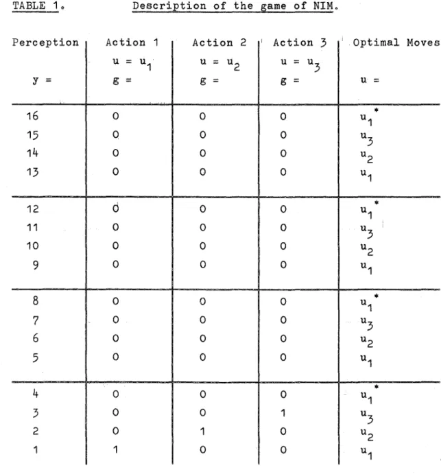
COMPUTING PROCEDURES FOR A

LEARNING MACHINE

A thesis presented for the degree of

Doctor of Philosophy in Electrical Engineering

in the University of Canterbury,

Christchurch, New Zealand

by

P.M. CASHIN, B.E.(Hons), M.E.(Dist.)

Ii) ,

ACKNOWLEDGEMENTS

I am deeply indebted to Professor J.R. Andreae who

has been my supervisor and has provided cont-inual

guidance, support and enthusiasm.

I have also had

valuable assistance from his methodically indexed

library of papers and bookso

Unfortunately, it is impossible to individually

acknowledge all the people who have helped me through

discussion, argument and cooperative effort during the

course of this worko

In particular the staff and

post~

graduate students in the Electrical Engineering

Department have contributed; many actively, all by

good willo

I am grateful to the University Grants Committee

for their scholarship which has supported me through

this work.

TABLE OF CONTENTS

CHAPTER 1:

INTRODUCTION

1-1

Introduction

1-2 Path Finding

1-3 Stochastic Learning Automata

1-4 Rote learning and Markov Process Theory

CHAPTER 2:

THE BANDIT ALGORITHM FOR MINIMUM COST

PATH FINDING WITH INCOMPLETE COST

'INFORMATION

2-1

Introduction

2-2 Proplem Statement

2-3 Illustrative Example

2-4 The Two Armed Bandit Problem

2~5

The BANDIT Algorithm

2-6 Some Comparative Results

2-7

Extensions to Path Finding

2-8 An Admissible Algorithm

2-9

Arc Cost Estimates

2-10 On-line Algorithm

2-11 Convergence Theorem

2-12 Applications of the BANDIT Algorithm

2-13 Results

CHAPTER

3:

STOCHASTIC LEARNING AUTOMATA

3-1

Introduction

3-2 Notation

3-3

Modified Linear Reinforcement Procedure

3-4 The BANDIT Algorithm

3-5

Environments with Perception and Performance

Measures

3-6 Results

3-8 Conclusions

References

CHA~ER

4:

ROTE LEARNING AND MARKOV

PROC~SSES

4-1

4-2

4-3

4-4

4-5

4-6

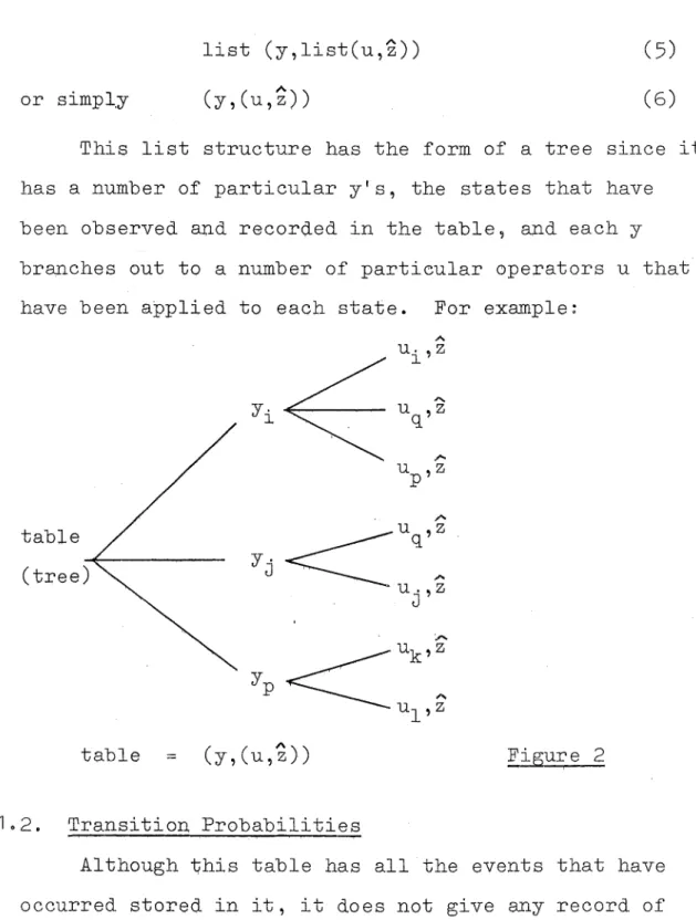
4~7

Table Building

Operator Selection Strategy

Planning from Rote Learning

Interaction as a Markov Process

An Example of Optimal Policy Failure

Stochastic Simulation

Operator Decision Procedure

4-8 Expectance Function

4-9 Operator Decision based on Expectance

4-10

E~pectance

Entry in the Rote Learning Table

4-11 BANDIT-EXPECTANCE MaQhine

4-13 Fox and Dogs Game

CHAPTER 5: CONCLUSIONS

5-1 Reinforcement Le~rning 5-1

5-2 Against Reinforcement Learning 5~2 5-3 Learning by Being Told 5-3

5-4 Why the Gap? 5-7

5-5 Grafting Learning Ability onto a Program 5-8

5-6 Summary of Main Points 5-10

APPENDICES

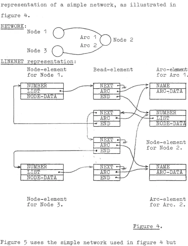
---,-.-APPENDIX A: LINKN~T: A Structure for Computer Representation and Solution of Network

Problems

Abstract

A-1 IJ;ltrQduction

A-2 The Basic Structure

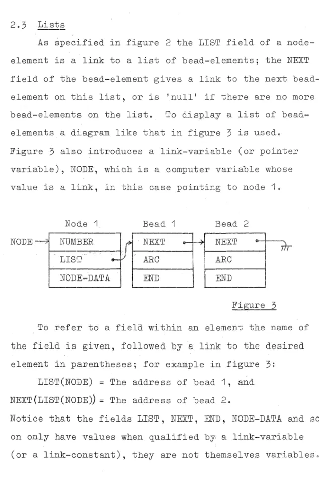
A-201 Graphs

202 LINKNET Elements

2.3 Lists

204 Access to apc attributes

205 Access to node attributes

A-3 Cre~tion of LINKNET

301 Construction of a LINKNET Structure

A-4 Applications of LINKNET

4.1 , Minimum length path finding

4.2 Finding Meshes and Spanning Trees

A-7

A-10

A-10

A-10

A-13

A-13

A-5 Conclusions

References

APPENDIX B:

GEAPHIC DISPLAY

SYS~EM -~.,...

B~1

Introduction

B~2 Bas~c

System

Requ~r8m~nts

B-3 The Edit Phase

-

D~rect

Draw Facility

-

Disp~ay

Language Facility

B-4

The Run Time Phase

- Display Order Inter

- Display File Editing

B-5

Editor~Interpreter

References

APPENDIX

_....,...-

0:

Analytic Calculation of BANDIT

Selection Probability for Normal Probability

Densitieso

APPEND~:

The BANDIT Algorithm in Heuristic

Search Algorithms,

Page

A-22

A-24

B-1

B-4

B-5

B-5

B-7

B-""10

B-11

B-15

B-19

CHAPTER ONE

1 - 1

CHAPTER ONE

1 - 1 INTRODUCTION

This thesis presents the highlights of work done

in the field of artificial intelligence - more

particul-arly machine learning. Artificial intelligence research

is accepted

[3J

as a wide ranging discipline, and no

attempt will be made to define or delimit it. The

areas of most importance to this thesis are, heuristic

programming, problem solving and associated learning

models.

Such important areas as pattern recognition are

scarcely mentioned in this thesis; this is not to imply

that such areas do not contribute to or supplement the

main theme of machine learning. It is simply that the

work reported has contributed no new concepts in these

areas, or linked them any closer to machine learning 0

The view has been taken that every learning machine

must face the problem of continually having to decide on

an action on the basis of some current set of collected

data and deductions. Each action can be thought of as

producing a 'value'. The problem is that the estimated

'value' of each action is based on the current data,

while each action may produce a 'side effect' of

1 - 2

This problem is exemplified by the 'Dual Control!

problem

[4]

and in its most basic form by the 'Two

Armed Bandit Problem' [2] 0 The Two Armed Bandit

Problem is first considered in Chapter 2, where the

BANDIT algorithm is first introduced. The BANDIT

algorithm is not only contributed as an algorithm for

solving the Two Armed Bandit Problem, but i t is

designed to be a basic mechanism in the learning

machine faced with the more complex and general problem

outlined above.

The heuristic that the BANDIT algorithm is based on

can be stated like this:

If one of a number of al ternati ves has a probability

'p! of beirig the best alternative, then choose this

alternative 100.p% of the timeo

To assess the probability 'pi of one alternative

being better than any other, it is necessary to know not

only the estimated mean 'valueo of each alternative but

also the probability density of these mean 'valuei

estimates. The BANDIT algorithm provides a concise

com-putational procedure to perform this decision processo

The applications, implementation and results from

using the BANDIT algorithm form a central core to this

The second contribution that plays a major part

in this thesis is the 'expectance' function. This

function is based on the 'expectation' used by

Andreae

(1)

and Gaines and Andreae [6

J

in the STeLLA

learning machine. It is similar to the expectimaxing

scheme proposed by Michie and Chambers

[9].

The purpose of the expectance function can be

thought of (for now) ,as .. a way of assessing an action's

long term 'value'. That is, not only is the immediate

'value' resulting from the use of the action considered,

but also account is taken of the future actions that

will become available, and of their expectance functions

or expected 'values i •

The development contributed by the expectance

function is its generality~ and equally important is its recursive formulation and on-line evaluation. The

expectance function is introduced near the end of

Chapter

3,

and is fully discussed ih Chapter 4.

Just as important as the BANDIT algorithm and the

expectance function themselves~ is their use in linking together and extending several distinct areas of

current research interest. The three main areas

con-cerned are:

Path finding (graph searching) - considered from a

particular point of view where incomplete information

1 - 4

Stochastic automata - with the introduction of an

extended problem class for these machines, and

Markov process theory and its use in the development

of a rote-learning table-based learning machineo

These topics are dealt with in Ohapter 2,

3

and 4 respectively. A brief 'over-view' of these topics is

given in this introductory chapter under sections 1-2,

1-3 and 1-4.

The function of the appendices is two fold. First

they contain some support material that is not

approp-riate 'in-line', but more important they contain some

originai material of their own 0 This material is not

included in the main body since i t is concerned with

computational tools that have been used (transparently)

to develop the algorithms and examples contained in the

main body. The two main topics in this class are:

10

A technique based on linked list structures that enables problems involving networks or graphs to be

im-plemented in a rather uniform manner. It is not so much

that the teChniques involved are in any way new? but

rather that the particular way of applying the techniques

to the network itself - rather than to the various

information structures that may arise in the course of a

particular problem - leads to structural and procedural

convenience. The ideas here have been developed in

1 -

5

used the technique on several power system problems.

20

A discussion of work done in implementation of a graphical display system for the Electrical Engineering

Department's EAI 640 computer. Although this display

system was develop~d from scratch in cooperation with

M.R. Mayson, the details of this work are not

consider-ed relevant to this thesis~ The philosophy developed is considered relevant however and is based on a large

effort devoted to establishing a framework for the

software.

1 - 2

PATH FINDING

Chapter 2 is concerned with a particular class of

path finding problems. Briefly these problems involve

repeated traversal of the minimum cost path that can be

found on the basis of current (incomplete) arc or path~

segment cost information. This is combined with the

upaating of the arc cost information for those arcs that

are traversed, on anyone path traversal. This problem

has been given the name 'on-line9 _{path finding.}

Chapter 2 is written in the form of a paper describing

an operations research technique for this class of

problem.

The presentation in Chapter 2 is thus rather closer

to the basic problem than if the sophisticated heuristic

1 - 6

intelligence workers had been explicitly employed. It

should be made clear however that by the very nature of I

graph searching in problem solving or game playing they

often fall into the 'on-linev _{path finding class.}

Oonsider for example a small board game where i t is

possible for a machine to search enough of the game

graph (tree) to establish that i t can not possibly win

if the opponent plays optimally. An example of such a

problem is considered near the end of Ohapter 4~ with

the French Military Game or Fox and Dogs.

In such situations we would like the machine to

make a move that maximized its chances of a win - that

is, try to put the opponent ~n a position where he is

most likely to blunder. Such performance is just not

possible by many successful tree searching programs,

since the basis of back-tracking up the game tree is a

mini-max strategy. On the oth~ band the efficiency of

the search (the work that i t involves) is very dependent

on the search strategy and this aspect has received

considerable attention [7][10J [11J.

A similar problem can occur in situations where a

complete search is not possibly by any strategyo In

this (normal) case the usual technique is to back-track

up the game tree from an estimation of the value or

merit of the various terminal nodes that have been

1 -

7

form is Samuel's checker player [12J.

An evaluation of

various search techniques is given by Slagel and Dixon

[14

J.

The problem arises not from the search and back up

procedures themselves but occurs as soon as the

estimates used for the value of each node are allowed to

be learned by the machine from its own experience.

In

fact as soon as the learning is directly derived from

the machine's own play we have an

'on-line'

path

finding problem.

Chapter 2 shows that without an

algorithm such as the BANDIT algorithm the learning

process in such cases is liable to get istuckO below

the optimal performance level.

The above comments apply equally well to problem

solving and theorem proving - except that in these cases

it may only be required to search once for a solution.

In other words the information update from one solution

to the next is not present.

In such cases the ion-lineo

path finding problem does not exist and the best

avail-able estimate gives the best that can be achieved.

There is no benefit from the

°

side-effect' of the

1 - 8

1 -

3

STOCHASTIC LEARNING AUTOMATA

Stochastic automata have recently been receiving

attention as models for learning behaviour and a survey

of this work is given by Fu (1970) [5Jo Chapter 3 is

concerned with this approach to learning machines,

starting with a brief introduction to the current

established work.

One recent scheme in particular [13J is then

developed and shown to be similar to a BANDIT algorithm

stochastic learning automaton, which is introduced at

this point. A benefit of this is that a proof of

con-vergence is given for the first automata scheme [13

J

and

a modified BANDIT automaton can be derived which falls

within the scope of this proof 0

Stochastic learning automata schemes are viewed in

Chapter

3

as procedureso For this point of view a

notation used in computer algorithm formulation is shown

as an attractive method for presenting the stochastic

learning automata procedures.

Finally the environment-automaton interaction is

generalized to enable this approach to tackle the class

of problems considered by several 'heuristic programmingi

schemes (for want of a better definitive). STeLLA [1,6J

1 -

9

1 - 4 ROTE LEARNING AND MARKOV PROCESS THE0RY

The basic memory strucpures and strategy used by

STeLLA were seen as similar to work on Markov process

theory developed by Howard

'[8J.

With this starting

point an attempt was made to bridge this gap by building

from the Markov theory towards the STeLLA strategy.

Unfortunately the complexity of the STeLLA heuristics

and special purpose parameters proved too great to allow

the theory to meet up with the STeLLA implementation.

By working in reverse a very basic STeLLA structure

was extracted in order to move closer to the Markov

theory.

This basic structure was (eventually) formed

into the BANDIT-EXPECTANCE algorithm as presented in

Chapter 4.

At this point the algorithm proved of

enough interest in its own right - and the road back to

STeLLA rather torturous - that the linking of the Markov

theory through to the BANDIT-EXPECTANCE algorithm was

considered as replacing the original objective.

Chapter 4 briefly presents the relevant Markov

theory and develops from this to end up with the

BANDIT-EXPECTANCE algorithm.

Throughout this development the

idea of a rote learning table is uS,ed to tie the

presentation together.

1 - 10

progresses from a simple record of events~ through to a more functional 9 control policyQ formo The structure of

the rote learning table is not too important in Chapter

4, except that i t contains the learning machineos long

term memoryo However, the format is developed in such

a way as to be extensible, and an indication of such

1 - 11

REFERENCES

1 Andreae, JoH., Learning Machines: A Unified View.

Encyclopaedia of Linguistics Information and

Control. Edo Meethan,AoRo and Hudson,RoAo

Pergamon Press, 1969.

2 Bellman,R. A Problem in the Sequential Design of

Experiments. SANKHYA Vol016, parts 3 and 4, 19560

pp 221-229·

3 Feigenbaum,E.A. Artificial Intelligence: Themes

in the Second Decade. Stanford Artificial

Intelligence Project Memo AI-67o Invited paper

IFIP68 Congress, Edinburgh, Aug. 1968,

4 Fel'dbaum,A.Ao Dual Control Theory I-IV in Optimal

and Self-Optimizing Control, Ed. Oldenburger,Ro

MoI.T. Press, 1966.

5 Fu,KoS. Stochastic Automata as Models of Learning

Systems. pp 393-431, Adaptive, Learning and

Pattern Recognition Systems, Edo Mendel~JoMo and Fu,K.So Academic Press, 1970.

6 Gaines,BoRo and Andreae,JoH. A Learning Machine

in the Context of the General Control Problem,

1 - 12

7 Hart,P., Nilsson9No, Raphael~Bo A Formal Basis

for the Heuristic Determination of Minimum Cost

Paths. IEEE Trans. on Syso Sci. Cybernetics,

July 1968, pp 100-1070

8 Howard,R.Ao Dynamic Programming and Markov

Processeso MIT Press 19600

9 Michie,Do and Chambers, R.Ao Boxes: An experiment

in adaptive control 0 Machine Intelligence 29

Edinburgh University Press 19680

10 Pohl?Io First Results on the Effect of Error in

Heuristic Searcho Machine Intelligence 5, Edo

Meltzer,Bo and Michie,Do Edinburgh University

Press, 1969, pp219~2360

11 Samuel,AoLo Some Studies in Machine Learning

Using the Game of Checkerso IBM Jo Reso Develop.

3 (July 1959), pp 211~229o

12 Samuel,AoLo Some Studies in Machine Learning

Using the Game of Checkerso II - Recent Progresso

IBM Jo Res. Developo 11, 6 (Novo 1967)9 pp 601~617o

13 Shapiro,I.Jo and Norendra,KoSo Use of Stochastic

Automata for Parameter Self~Optimization with Multimodal Performance Criteria. Trans 0 IEEE

Systems Science and Cybernetics, Vol. SSC-5 No04,

October 1969, pp352-3600

14 Slagle,JoR. and Dixon,JoKo Experiments with some

CHAPTER TWO

2 - 1

CHAPTER TWO

2 - 1 INTRODUCTION

The problem of finding the minimum cost path

through a graph (network) of interconnected nodes where

the arcs? or node interconnections have associated costs

has been solved in many wayso The applications of this

problem range from transportation routing problems

[1]

through automatic control, [2] to artificial

intel-ligence research

[3]

0

2 - 2 PROBLEM STATEMENT

Existing algorithms cannot satisfactorily tackle

certain problems having incomplete cost informationo

Here we attempt to solve a class of problem that we

have termed ion-lineQ

0 These problems have the

follow-ing characteristics:

a) The graph is to be traversed from a start node to

one of a set of goal nodes N timeso

b) The costs associated with the arcs are not fully

known and may be stochastico

c) Information gained from each traversal of the

graph is to be used to update the corresponding

arc cost estimates 0

d) We wish to minimize the total cost incurred by the

2 - 2

In descriptive terms the problem is that of decid~ ing whether to travel a known path or to spend money in

exploring for a short cut. It is clear that a 'search

for the best pathQ policy may well precede a 'use the

best path that has been foundo policyo

-THE O~-LINE PROBLEM

Traverse graph from start to goal.

J

Path Cost

=

sum of costs of arcs traversed.

1

C=UPdate arc cost estimates

~

'.J

-Select the next path to traverse on the

basis of the current arc cost estimateso

The object is to minimize the total cost over a number of traversals of the grapho

2 -

3

ILLUSTRATIVE EXAMPLE

To illustrate the on-line path finding problem

consider the case of a transport operator who has a

contract to transport goods between city A and city Bo

The contract is such that time is the important factor,

2.- -

3

city A to city B is the travel time rather than the

mileage or fuel cost or anything else.

In this example the arcs are the separate lengths

of road that may be travelled as part of some path from

A to B. The arc cost is the travel time for an arc.

Notice that the arc cost is a random variable since

hills, bends, traffic density and so on will all

affect the travel time. Notice also that a reasonable

apriori estimate of the mean travel time is available

using road maps and so on.

Every time the transport operator runs an

assign-ment from A to B he is able to update his cost eSimates

for the roads (arcs) that he chose to travel.

Consider the simple case where there are only two

possible paths from A to Bo Assume that the paths have

costs uniformly dis.tributed in the range 0.7 to 008 and

008 to 0.9 respectively. In our ignorance we may well

assign apriori estimates of 1.0 for the cost of each

route. Making an arbitrary choice we proceed by the

second path on the first occasion and find i t better

than the apriori assumption. From this moment onwards

the simple strategy of travelling the minimum

(estimat-ed) cost path, would never get around to trying the

other route, although quite obviously i t is better.

A heuristically derived algorithm - the BANDIT

2 - 4

problems. The BANDIT algorithm accepts apriori

estim-ates not simply as a mean cost but as a probability

distribution for the mean costo

Although the BANDIT algorithm is not guaranteed to

be optimal in the sense that it will minimize the total

cost over a number of traversals, i t is shown to be

very near optimal for simple problems and is

computat-ionally feasible for large problems. All known methods

for optimal solutions are impractical (or even

currently impossible) for large problems, but they can

be used on small 'artificialv _problems.

The optimal solution for simple problems will be

given by use of Bellman's method [~? which was

propos-ed for the

'two

armed bandit problem' 0 This problem

(to be described in the next section) can be taken as

equivalent to the two path problem described above by

considering the two slot machines to be the two paths?

and the payoff probability as relating to the path cost.

For example, a slot machine ~YQff probability of

0075

can be interpreted as

0025

mean path cost (normalized).

Note that the two armed bandit problem (next

section) is considered because it is only for this

simple case that Q£timal solutions can be computedo

The BANDIT algorithm is then described and shown to

2 -

5

2 - 4 THE TWO ARMED BANDIT PROBLEM

The simplest form of the path finding problem is

equivalent to the two-armed bandit problemo This is a

classical mathematics problem that is still not

com-pletely solvedo The basic two-armed bandit problem is

outlined below:

Suppose that we have two slot machines in front of

us, one with known properties and one with unknown

propertieso When the handle on the first machine is

pulled, there is a known probability, s, of receiving a

dollar; when the second machine is played, there is a

fixed, but unknown, probability or success, ro

The process assumes the following formo We try

the second (unknown) machine a number of times to be

determined by the outcomes, and then* decide to use the

first machine from then ono

The object is to maximize the expected value of

the criterion function:

R

a

n

z

n

where 0

<

a

<

1 is a discount factor and zn represents

the return obtained on the nth trial.

This criterion function enables the problem to be

treated as an unbounded process with discount factor, a,

rather than a finite sequence of choices where we have

2 - 6

N trials.

Bellman's dynamic programming approach [4] to this

problem gives a computational method that is feasible

for the case of one unknown and one known payoff

prob-ability to choose between (as above).

For multiple

choice problems the co-mputation would quickly become

impractical.

No analytic solution has been derived for

an optimal policy.

Bellman defines:

f

(s)

=

the expected return obtained using an optimal

mn

policy for an unbounded process after the

second (unknown) machine has had m successes

and n failures.

It is assumed

[4J

that the probability

distribut-ion Fmn (r) ,r/1'or r in

[0, 1J

after m successes and n

fail-ures, is updated from the apriori eSimate.

Let the

expected value of Fmn(r) be Pmn0

The basic functional equation can now be written,

Max

s/(1-a)

Bellman gives an existence and uniqueness theorem

that enables the above equation to be solved by a

Bellman's method has been outlined above since i t

shows the difficulty involved in this problem; also i t

provides a computational method for the optimal policyo

These optimal policies will be compared with the results

from a heuristic algorithm which is described belowo

2 -

5

THE BANDIT ALGORITHM

We will leave the two-armed bandit problem for a

moment in ord~r to set out a heuristic decision proced-ure that will be central to the rest of this chaptero

The heuristic that the BANDIT algorithm is based

on can be stated like this:

If one of a number of alternatives has a

probab-ility 'pi of being the best alternative, then choose

this alternative PQ100% of the timeo

To assess this probability of one alternative

being better than any other, i t is necessary to know not

only the estimated mean costs for each alternative but

also the distribution probability of these mean costso

The apriori distribution to be used is not an

objective probability corresponding to some random

ex-periment, but rather degrees of belief based on prior

analysis of conditions relevant to the particular

prob-lem. Thus apriori distributions including a zero

prob-ability for some range of values imply a complete belief

2 - 8

common apriori distribution would be a normal

(Gaussian) form, the variance reflecting the confidence

in the mean estimateo

Consider the case of only two alternatives as in

the case of two possible paths from A to Bo If the

cost of one path is estimated to be 0085 with variance

of 0015, and the other path is ~nown to have a mean cost of 0075; roughly, the BANDIT algorithm will give

the 0075 cost path preference about 84% of the timeo

The other 16% of the traversals are used to establish

a better estimate of the 0085 estimated mean cost path

-making sure that it really is a greater cost than 00750

As we become surer the variance drops and the 16% falls

lowero

We will now frame the BANDIT algorithm in a more

formal and precise manner:

Let S1~S2,S3?00,SN. be N alternatives 0 We must

select one of these and the estimated mean cost of

selecting S. is x. 0 Let f.(x) be the probability

dis-l l l

tribution for x., i t is to be understood that this is

l

the current distributlon and updating occurs to fi(x)

after S. has been selected and its cost measuredo The J.

measured cost is treated as a sample from an unknown

distribution g.(x) and the expected value of f.(x) is a

~ ~

mean estimator for gj,(x) , The object is to minimize

From the f.(x) we can calculate the current

l

probability that the cost of S. will be less than any

l

of the other alternatives, p(x

i = min {xj ij=1,2,oooN,'}).

BANDIT Algorithm

Select Si with a probability P(Si) such that

p ( S.) = P ( x . ;.:: min { x . ; j = 1 ,2 , ° ° • ,N}) Q

l l J

The direct computation of p(S.) would require

l

evaluation of the integral:

0<)

p(s.)

=1

I T ( 1 - F.(x))of.( ) d

l 0 j

I

i J l X ° X

X

F.(x) =

1

f.(x)odx; the cumulative distri-J 0 J

Where

bution (see Appendix C for details)o

Fortunately since we only need to select one of

the possible strategies,

Sj~{Si}'

we can employ a Monte

Carlo type procedure to avoid calculating P(Si) for

each i, i. e ° { P(Si)

J.

The procedure is to take a set

of random samples, {y.; i=1,2,oo.N)' where each y. is a

l . l

random sample from the probability distribution fi(x)o

If the minimum of this set is Yj' where Yj =

min { y i : i=1 ,2, 0 • oN}, then select strategy S j ° Notice

that unlike normal Monte Carlo procedures only one set

2 - 10

procedure were repeated a large number of times then

the set of probabilities of selection for each strategy,

{P(Si)}' could be evaluated.

An additional simplification can be made in the

procedure by assuming that the f.(x) are all normal

dis-1

tributions. This will usually be an acceptable

assump-tion since the central limit theory proves that the

dis-tribution of a mean estimator will tend to be normal as

the number of samples becomes large~ regardless of the form of the parent populationo Further, if the parent

population is normal in its distribution then the

dis-tribution of the mean estimator will always be normal.

2 - 6 SOME COMPARATIVE RESULTS

In order to illustrate the operation of the BANDIT

algorithm we have compared its performance on some two-·

armed bandit problems with the optimal solution

(computed by Bellman's method) 0

The optimal solution involves a switch from the

un-known machine to the un-known one after a particular

sequence of successes and failures. For any given

num-ber of trials, the probability of different sequences of

success and failure can be computed and hence the

prob-ability of a switch to the known machine.

The BANDIT algorithm has a probability of selecting

either machine that depends on the sequence of successes

2 - 11

above we compute for each given number of trials the

probability of each possible sequence of success and

failure, and hence the overall probability that the

known machine will be selected.

The above procedure has given the results for

both the optimal solution and the BANDIT algorithm in

the form of a probability that the known machine will

be selected after any given number of trials. These

results can be directly compared and this is done in

figure 2. Discount factors, a, of 005 and 008 are shown

for the optimal policy. Both methods used the same

apriori eSimate for the unknown machine payoff and also

the same updating procedure. The distribution of the

payoff probability for the unknown machine was assumed

?ROB.

of

~~8

I

~

___

~-.r

r- _

-.J

r-

~

r-:;.

:2~]~~-~-=~;~~

OPTIMAL a=O

0

8

: 0

a=Oo5

I •

t

BANDIT ALGORITHM

I I

.J I '

I I

I •

PAYOFF PROBe

M/C I

known MfC II unknown

I :

0.25

.= Oe10

o

~--~--~---~----~--'i

TRIAL

o

10

20

30

PROBe

of

M/C

I

100

PAYOFF PROBe

M/C

I known

0.25

M/C II

unknown

= 0.30

;

\

BANDIT ALGORITHM

OPT IMAL a=O 0 8

~I

.

a=O 051

....r---~~ ... _ _ f

J

i - - ~ - ~ -t:J -IU"...,,~=-.rr~ - -~.

: :~ - J - ' - - - • ~-i

I

I

O

_~ I-__ -LIL; ____ ~---_,._---₁

_TRIAL

6

10

20

30

Figure 2

PROBe

of

M/C

I

1 0

OPTIMAL a = 008

.j-a =

rO~~;j

__

! - - -n-"'_::::-I

r--~-.-

-Rd-

'!=- - - ) ,

r-~.r-~.-...i

BANDIT ALGORITHM .

...J I I

I i

I I

I i '

PAYOFF PROBe

M/C

I known

M/C

I I unknown

O+---~----~---~---,

TRIAL

o

10

20

30

PROBe

of

M/C

I

1001

PAYOFF PROBe

M/C

I known

M/C IT

unlmown

1 ',.

BAHDIT ALGORITHM

0.25

0.40

005

1 '"

OPTIMAL a=008

1

~

a=0·5

1

~

-1 ;_ ~-:'~_j-.~ _ _ _ _ _ _ _

',,----. ~-~ - -~T:L~

-I t [ \ )

O~---~!~;----~---~---~I

TRIAL

I

2 -

7

EXTENSION TO PATH FINDING

It is not practical to calculate an optimal

solut-ion for even a small on-line path finding problem. We

can appreciate this by considering the extensions that

need to be made to the two-armed bandit problem:

1. Extension to an m-armed bandit problem. (m al

ter-native paths).

2. The cost of all m paths may be unknown apriori.

30

The traversal of one of the paths allows updating

of a set of arcso These sets of arcs for each of

the m paths are not necessarily mutually exclusive.

4. It requires considerable calculation to evaluate

the set of arcs that form the minimum cost path

(on the basis of the cost estimates). In general

i t is impracticable to list all of the m

alternat-ive paths an~ their costs.

Point 4 leads on to the procedure that will be used

to find a path through the network.

2 - 8 AN ADMISSIBLE ALGORITHM

We shall use the definition in

[5J

for an admiss-ible algorithm, which (briefly) is any algorithm that is

guaranteed to find an optimal path from the start node

to a .. goal node. Dynamic Programming

[1]

and the A*

2 - 14

An optimal path from node i to node j has the

low-est cost over all possible paths from node i to node jo

An admissible algorithm considers only the set of arc

costs it has to work with so that the optimal path that

it finds is more correctly the current-optimal patho

It is only optimal on the basis of the current arc cost

estimateso

In the on-line path finding problem the

current-optimal path on the basis of the current arc cost

estimates may not be the true minimum cost path (the

optimal based on the, unknown, true mean arc costs)o

This fact can cause the admissible' algorithm to

I

sit

i

on one particular path each time it is used during the

course of an on-line path finding problem, even though

this path may not be the true-optimal

0

The feedback

that comes from the measured arc costs between each use

of the admissible path finding algorithm (used to

up-date the arc cost estimates) may not help simply because

only those arc costs on the current-optimal are being

measuredo

This failure of an admissible algorithm in

2 -

9

ARO OOST ESTIMATES

We will denote the cost of the arc i-j from node i

to node j as c .. , and its estimate

c. ..

The

C ..

are

lJ

.

lJ

lJ

updated every time arc i-j is traversed. A form of

stochastic approximation can be used;

c. .

~ a.

c. .

+ (1-a). c. . i

lJ

lJ

lJ

where c .. I is the arc co st as measured, and 0 ~ a .. ~ 1. *

lJ

'

If c

ij is known to be deterministic, use a

=

o.

More sophisticated forms of this process can be found in

[6J.

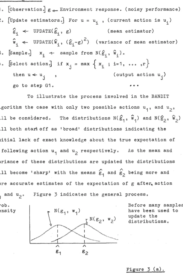
Figure

3

illustrates this process, and shows how the variance of the estimate can be maintained in a similar

manner.

We will use O. to denote the cost of path i, one of

l

the set of possible paths from the start node to a goal

/'.

node. O. will be the estimate of 0.; i.e. the sum of

l l

c ..

for all arcs i-j on path i 0

lJ

2 - 10 ON-LINE ALGORITHM

The on-line algorithm applies an admissible

algor-ithm at each traversal under the on-line conditions 0

A

'" A

If O.

<

O. for all i

I-

j, and for simplicity

J l

OJ

=

OJ' then the on line algorithm will select path j

A

to be traversed. However, if Ok

>

OJ and OJ> Ok for

2 - 16

some k then the on-line algorithm will have converged

onto a non-optimum path since C

k

<

Cjo

2 - 11 CONVERGENCE THEOREM

The on-line algorithm is guaranteed to converge

onto the optimum path under the following conditions:

A

c ..

1J

A

c ..

1J

c .. -7

c ..

1J 1J

for all i-j

as arc i-j is repeatedly

traversedo

The proof of the convergence theorem follows from

contradiction of the hypothesis of convergence onto a

non~optimum or non-convergenceo

If we cannot satisfy the conditions of the

conver-gence theorem we have shown that the use of the on-line

algorithm will not always be successful. The BANDIT

algorithm is proposed to overcome this difficult yo

2 - 12 APPLICATION OF THE BANDIT ALGORITHM

We have shown that the BANDIT algorithm performs

well in comparison to the optimal solution for some

simple two armed bandit problems, which is the basis of

the on-line path finding problem. There is no known

method that is practical for computation of the optimal

solution for the more complex on-line problem. The

BANDIT algorithm (which requires only modest

solution. Instead we must rely on the vreasonablei

nature of the algorithm - as with most heuristic

proced-ureso

We have found proof of convergence for a modified

form of the BANDIT algorithm in terms of the theory of

variable structure automata, [8Jo This is discussed in

the next chapter (Chapter

3).

This chapter however

will rely on an example to support the worth of the

algorithm.

The application of the BANDIT algorithm to the

on-line path finding problem requires:

10

A procedure to maintain and update a distribution

for the mean estimator for each arc cost~ If

advantage is taken of the fact that by the central

limit theorem this distribution will tend to be

normal, then only two parameters (mean and

var-iance) will be required for each arc cost

estimat-iono One possible procedure for updating these

parameters has been outlined in figure

3.

20

A procedure for obtaining a random sample from each of the mean arc cost e~mator distributions 0 There

are many random number generators available

-again the computation is simplified if a normal

distribution is assumed.

30

An admissible algorithm that can be applied to the

2 - 18

a standard minimum-cost past finding program to

hand and this could be used directlyo

The operation of these three procedures is shown

in figure

40

The application of the BANDIT algorithm to

heur-istic search algorithms used in artificial intelligence

research is discussed in Appendix Do However, the

notation for algorithm presentation developed in

Chapter

3

is used,so that a detailed study of Appendix D is best left for the presento

2 - 13 RESULTS

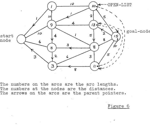
The small network shown in figure

5

was used to

demonstrate the BANDIT algorithm as applied to the

on-line path finding problemo The true mean arc costs for

this example are shown in figure

5

and the true optimal

path is shmn with the dotted lineo The apriori arc

cost estimates were all taken as equal so that the

apriori current optimal path will be either around the

top or around the bottom in figure

50

Two other methods apart from the BANDIT algorithm

were applied to the same example 0 One was the on-line

algorithm which in 'this case will not have the

condit-ions specified in the convergence theorem satisfiedo

The results from this show the trap of applying a

Probability

Unknown

Distribution

~----+---:>~ c .. c· .

lJ

lJ

~ean estimator distribution:

Probability

Approxo Normal Distribution

_ Estimated

--~----A~i---?;>Pmean cost

c ..

lJ

Lgure

3

Each traversal of arc ij lncurs a cost c· · 0

lJ Cost at time t = c .. (t) .

lJ

Estimate of c .. (t) -C . . (t) 0

lJ lJ

Variance of ~ .. (t) = v .. (t).

lJ lJ

S.T.Do of ~ .. (t) d . . (t).

lJ l J ·

Update

~ .. (t)

of mean and variance for the cost of arc ij.

lJ v . . (t)

lJ

d . . (t) lJ

a.~ .. (t-1) lJ

aov . . (t-1) lJ 1

(v . . (t))2

lJ

m

+ (1-a).c .. (t); lJ

+ (1"':'a)o(-C . . (t) lJ

2 - c .. (t))

,lJ

m = the number of samples,

m is limited to (1+a)/(1-a), the moving average sample

the exponential smoothing

that if a=(m-1)/m, and m lS number that is equivalent to

equation, Brown

[7

Jo

Notice

the total number of samples available, then the above

equations reduce to the standard (classical) mean and

variance estimators 0

I~

Mean Arc Cost Estimates _{Random Samples}

Prob 0

-Mean 1

A

~--~---~~ Estimate

prObej,_---'---;

_/f'''.

/

~.

\, Mean 2 : .... ~ ;;. Estimate

I

Probo

THE BANDIT ALGORITHM APPLIED TO ON-LINE

PATH FINDING.

Apply Dynamic Prog. or A* algoritbm

/. Travel Minimum Cost Path

(Any minimum cost path finding algoritbm may be used).

1t

Update Estimates

~ ----~~---~

Figure 4

I~

I

2 - 21

problem. The other method was an algorithm that

selected a path with probability inversely proportional

to the relative cost of the patho

Figure 6 has a graph of the results expressed as

incremental costs (total cost incurred divided by the

number of trials) 0 These graphs can be viewed as a

form of 'learning' curve 0 T.he BANDIT algorithm is the

only one to converge onto the true minimum cost patho

The same results obtained from the BANDIT algorithm

are shown in a different form in figure

70

Here the

probability that each of the possible paths will be

chosen is graphed against the number of trials (plotted

START

Figure

5

SMALL NETWORK EXAMPLE

True Mean Arc Costs

Apriori estimates: All arc costs

50

Std deviation

30

True arc costs: As shown above with

Std deviation

=

10.

GOAL

igure 6

250

200

150

100

50

Incremental Cost Total Cost Number of Runs

Probability of travel inversely proportional

r

to estimated cost.

/

I.

I

Traverse minimum

~

cost path (estimated)

BANDIT Algorithm

-

--

-

-

-

-

- - - -

-

-

-

- -

~

-

-

- - -

- - - - - - -

-Minimum Path Cost

o

+---,---,---r---r----~--_.---_r---~

o

20 40 60 80

Number of Runs

100 120 140

Probo of Traversal 100

'/

0.8

True Minimum Cost Path

r

Apriori Minimum Cost Patho

I

-

2nd to Minimum Cost Path.

004 -\.

I'

i

I

I

002

1

i

BANDIT ALGORITHM

-EXAMPLE RESULTS

I

Figure

7

o

1----~~--- ~~

~~~--_, I~

2 - 14 CONCLUSIONS

A class of path finding problems that involve a

simultaneous maximization of information gain and

minim-ization of incurred cost has been described as the u

on-line' path finding problema A heuristically derived

algorithm - the BANDIT algorithm - is proposed to tackle

these problems a

Simplest form of the on-line path finding problem

is the two armed bandit problemo An optimal solution

for this problem is compared with results from the

BANDIT algorithmo

The application of the BANDIT algorithm to the full

on-line path finding problem is then outlined and some

results given for a small example problemo

The computation of the optimal solution for the two

armed bandit problem is an iterative procedure requiring

considerable computation 0 The extension of this method

to the on-line path finding problem is not practical 0

The BANDIT algorithm on the other hand requires very

little computation if the method outlined is followedo

A convergence theorem with the particular conditions

under which a standard path finding method (such as

dynamic programming) can be successfully applied to the

on-line path finding problem is given 0 The BANDIT

algor-ithm can however be applied to any standard procedure

2 - 26

problems that can be successfully tackledo

No discussion has been given for the case where the

random arc costs have time variable statistics (such as

drift in the mean cost of some arcs)o Preliminary

results show that the BANDIT algorithm is capable of

tackling such problems and the methods suggested leave

this possibility openo There is no known optimal

solut-ion to this class of problem even for the simple

two-armed bandit situation.

A convergence proof for a modified form of the

BANDIT algorithm has been found in terms of the theory of

variable - structure automata

[8]0

This will be

REFERENCES

1 Kaufman, Ao, Graphs Dynamic Programing and Finite

Games, Academic Press, 19670

2 Bellman, Ro,

&

Kalaba, Ro, Dynamic Programing and Modern Control Theory, Academic Press, 19650

3

Slagle, JoRo

&

Dixon, JoKo, Experiments with some Programs that Search Game Trees, JACM Volo116, No02

April 1969; pp 189-2070

4 Bellman, Ro, A Problem in the Sequential Design of

Experiments, SANKHYA Vol0116 pt.

3

&

4, 1956; pp 221-229.

5 Hart, P.E., Nilsson, N.Jo

&

Raphall, B., A Formal Basis for the Heuristic Determination of Minimum Cost

Paths, lEE Trans, on System Science

&

Cybernetics,

SoS,C. 4 Noo 2 July 1968; pp

100-107.

6 Fu, KoSo, Stochastic Automata as Models of Learning

Systems, Computer

&

Information Sciences II, Ed. JoTo

Tou, Academic Press, 1967; pp

177-1920

7 Brown, RoGo, Smoothing forecasting and prediction of

discrete time series, Prentice Hall, 19620

8 Chandrasekaran, Bo

&

Shen, DoW.C" On Expediency and

Convergence in Variable - Structure Automata, IEEE

Trans. on Systems Science

&

Cybernetics, March 1968,

CRAFTER

THREE

3

~ 1

3 - 1

INTRODUCTION

This introduction gives a brief survey of the

development of stochastic learning automata and develops an

algorithmic notation for the concise description of these

schemes. Following this9 a new development called the

BANDIT scheme is described and some of its advantages

considered.

The class of problems considered₉ or the environment

for the stochastic learning automaton9 is then extended to a

much wider problem class that cannot be tackled by the

automata schemes described₉ but has been considered in the

field of 'heuristic programmingQ _{for learning machines as}

robots and game players. The BANDIT automaton is extended

by the development of an iexpectanceQ _{function in order to}

tackle this extended problem classo Illustrative results are

then given"

A more detailed historical development of ~ost of

the material outlined here ~an be found in Fu (1970) [11]

The behaviour of a finite state (deterministic)

automaton operating in a random environment was first studied

, '

by Tsetlin

(1961) [15]

A simple block diagram of the system is shown in figure 10

u €

Random ' U

~

Environment ]

Automaton

"""

Y € Y

3 - 2

The response of the'environment can be y = 19

called a penalty response9 or Y

=

0 called a nonpenalty or

reward responseo Tsetlin characterised the environment by a

vec t or C

=

(C 1 9 00. 9C ) where~

r

C.

=

Pr ( y ( t)

=

1

I

u ( t)

=

u.) j

=

1 I

0..

9 r ( 1 )

J J

u(t)

=

automaton's output or action at time t9

yet)

=

the environments response to this actiono

C.

J

=

the probability of a penalty response for action Ujl

and (1-C.) = the probability of a reward response.

J

A stationary random environment is considered

which means that the C. are all constant values over time,

].

Following Tsetlins approach Varshavskii and

Vorontsova (1963) (16J have used a variable structure automaton

as a model of a learning system operating in a random

environment. Their approach was to modify the state

transition probabilities in such a way as to minimize the

1

probability of a penalty response. If p .. (t) is the

l.J

transition probability from Automaton state qi to state qj

for the environment's response Y=Yl, at time t, then~

r

1

Pij (t)

=

1 for all i and t. ( 2)

j= 1

The idea i~ to minimize the probability of a

penal ty response by a decrease of p .. 1 every time a transition

l.J

from state q1 to qj due to response

Y1'

is followed by a penalty responseo

1 follows9 then Pij

If however a nonpenalty or reward response

3 = 3

state transition probabilities constitutes a transition

probability update procedure. An admissible transition

probability update procedure must be such that (2) applies

after every update.

Fu et al (1965~1966)

[7J

[8]

hav~ extended Varshavskii and VorontsovaVs work

06J

to the more general case where:

1. Instead of updating the transition probabilities, any

convenient probability function is treatedo (The total

state probabilities for example).

20 The performance of the automaton is measured not by a 1

(penalty) or 0 (reward), but by any value between 0 and 1.

The system now looks like figure 20

-\

~ _/ Random

Environment

J

Y E Y

u E U Performance

Evaluation

' - - / '

I

Automaton _'"

Z

, Figure 2.

-Let the probability of the automaton taking the ith

decision, choosing the ith action9 or being in the ith state

be p. 0

~ The index i=19 000 ,r 9 ~here r is the total number of

possible (quantize~ parameter settings, or the number of states

of the automaton.

written as:

A linear reinforcement algorithm to update p. can be

~

1

p. (t+1) ::

1

Where 0 < (,)\ <. 1 ~ 0 ~. z. (t) ~~ 11 and ).

r

i:::1

1

z, (t) ;:: 1.

).

3 ~ 4

p.l(t)

=

the probability of action u. due to input (environment

). J.

response) Y11 at time to

1

z. (t)

=

a performance measure evaluated from the environments ).

response to action u.

Cu.

due to y]) at time t.

) . ) . .

A slightly different viewpoint is to consider the

use of a learning automaton as a hill climber to maximize or

minimize some performance measure. The environment can now

be considered as providing an output that is a performance

measure I(u.) for action or parameter setting U.c

). ). The output

from the environment that is available to the automaton is

denoted g(u.) and this will be a noisy observation or

).

measurement of I(u.).

). The expectation of g(u.) will be the ).

actual performance measure for action u.,

l(u.)Q

). ). The aim of

the automaton is to give an output or parameter setting u _op t

such that I(u t) is an extremumo

op From now on only a maximum

will be considered , in contrast to the minimization of a penalty

probability considered previously.

Shapiro and Narendra (1969) (14J have considered this

use of a learning automaton as a hill climber in situations

where only noisy measurements of performance are available and

the performance hill may be multi-modal. Their scheme is

outlined below because it comes closest to the BANDIT algorithm

that is to be described 1aterl and results from the scheme are

3 - 5

An important point about the scheme proposed by

Shapiro and Narendra is that it can achieve optimal performancej

whereas the schemes previously outlined can₉ in genera1₉ only

achieve expedient performance. Convergence and expediency

have been considered for several learning procedures by

Chandrasekaran and Shen

(1968) [5]

Expediency in the context of hill climbing9 is said to occur when for;

k=1j ••• r 9 klj (4 )

in the limit as t ~. 00 , the probability p.(t) of selecting

J

action j is greater than Pk(t), in either a deterministic or

probabilistic sense as the particular case may apply •

. Optimality is a stronger result than expediency

and it requires that;

1 im p. (t)

=

1

t -cO _J

and

1im Pk(t)

=

0 for k;lj t-+«>

Before giving more details of particular procedures

some notation will be introduced to clarify the presentation.

20 NOTATION.

An algorithmic notation is used because it eliminates

an explicit reference to time which is a particular advantage

for variables that are updated but not necessarily updated

every time interval. More than this it is desirable to give

a clear indication of the uformv _{of a procedure}

j without

restricting the procedure to a particular set of rules. The

3

=

6

work of Knuth (1968)[10J and is introduced belowo

Consider for example the statement:

A 1 0 fUpda te]

Here ~ is an estimate (indicated by the hat) of a variable Xo

Whenever the step A1 is carried out ~ is updated by

replacing its current value by the evaluation of the

expression to the right hand side of the arrow (~)o The phrase in the square brackets at the start of the step~ in

this case [Update] is s brief summary of the principal content

of the stepo There will sometimes be parenthesized comments

at the end of the steps; in A1 the range for alpha is a

commento

Now consider a more detailed procedure:

B 1 [I ni t i al i z e

a

at

+- 0 9 k -+' 1 0

B2 [ObservationJ X <- observationo

B3. [ppdate mean estimatorJ

'i

-1.-Q(~ + (1=c{)xo

B4 [CountJ k <~. k+19 <X «- (k=1)/k9 go to step B20

This B=procedure is simply a method for evaluating

the classical mean of a set of observations (samPles) xJ.

Note that there is no final answer9 the procedure is qon line q

and simply maintains an estimator ~o

k

A 1

~--x = X·

k L... _j::::1 j

( 6)

If however IX is a fixed constant:

3 - 7

C2 [Input.] X +·observationo

C3 [UPdate mean estimate~

x

4-- 0\, ~ + (1- O<)X9 go to C20

The C-procedure is a moving average or exponential

smoothing procedure9 Brown (1962) (2). The procedure may also

be interpreted as a linear reinforcement learning procedurej

Bush and Mosteller (1958) [3].

In a similar manner we can maintain some estimator

of the variance of observations Xg written:

D1 [Variance updateo]

~

-4-

o(~

+ (1-(1{) <£_x)2 0 (0<0(:;;1)0

And for the variance'of the mean estimator:

E1 [Mean variance updateJ A W <+- B .A V

I (p~ 1/number of samples)

Where for a classical estimator of the variance

of the mean, ~ would be 1/(k-1) j k being the number of samples

or observations of Xo

Now the step A1 by itself can be interpreted as

part of a B-procedure or part of a C-procedure or any similar

procedure where 0< may be a more complex function Fu (1967) [9]

However instead of leaving a step like A1 in an

algorithm where ~ is not specified the notation:

~ ~ UPDATE (

x

9 x).~ will be used 0

It is to be understood that any of the procedures

described or referred to above are appropriate for the

UPDATE functiono For that matter it may be any procedure to

do a similar job under the particular circumstances that may

3 - 8

3. MODIFIED LINEAR REINFORCEMENT PROCEDURE.

The modified linear reinforcement scheme developed

by Shapiro and Narendra [14J will now be described in terms

of the notation discussed above. Remember that

g = the environments response to the automaton9s action U ,

u €. _{{ u}

i 9 i= 1 i • 0 0 9r } 9 U is a noisy performance measureo A

the probability that

Pi = the automaton will select action ui9

the hat indicating that these probabilities are estimates

of the probabilities that will give optimum performanceo

F10 [Observation 0] g ~ observed environment responseo

F2. [Reward set up

J

Let g.

=

max {g.

J 1.

. 1 . 1

~ 1.= 9 0 0 0 9 r

f

0

If 000 ,r • (No reward.)

A

Else if g ~ g. I and u = U. 9 (The last action was u.)

J 1. 1.

o (Reward i th action).

F3. [Record performanceJ if u

=

u. (Last action was u.).

1. 1.

then + (1- iT) g

k. ~ k. + 1 ,~4-( k. = 1 ) /k .•

1. 1. 1. 1.

F40 [Update.] if z. := 0, i=1, 0 0 0 9r I then go to F5.

• . 1.

(No update unless reward) 0

A A

Else p. -+-- o{p. + (1= C<)z. , for i=1, 000 ro

1. 1. 1.

(ct.=constant,O<0<.<1).

F50 [Select actionJ Select action u. with probability p. 0

1. 1.

u -+' U. (execute action u.)

1. 1.

go to step F1. • ••

A

In the above procedure g. is a mean estimator for

1.

the performance measure resulting from the use of action u. 0