University of Warwick institutional repository: http://go.warwick.ac.uk/wrap
This paper is made available online in accordance with
publisher policies. Please scroll down to view the document
itself. Please refer to the repository record for this item and our
policy information available from the repository home page for
further information.
To see the final version of this paper please visit the publisher’s website.
Access to the published version may require a subscription.
Author(s): Colm Connaughton, R. Rajesh, Oleg Zaboronski
Article Title: Constant flux relation for aggregation models with
desorption and fragmentation
Year of publication: 2007
Link to published article:
http://link.aps.org/doi/10.1016/j.physa.2007.04.074
arXiv:0708.2139v1 [cond-mat.stat-mech] 16 Aug 2007
Colm Connaughton,1,∗ R. Rajesh,2,† and Oleg Zaboronski3,‡ 1
Center for Nonlinear Studies, Los Alamos National Laboratory, Los Alamos, NM 87545, USA 2
Institute of Mathematical Sciences, CIT Campus, Taramani, Chennai-600013, India 3
Mathematics Institute, University of Warwick, Gibbet Hill Road, Coventry CV4 7AL, UK (Dated: June 2, 2011)
We study mass fluxes in aggregation models where mass transfer to large scales by aggregation occurs alongside desorption or fragmentation. Two models are considered. (1) A system of diffusing, aggregating particles with influx and outflux of particles (in-out model) (2) A system of diffusing aggregating particles with fragmentation (chipping model). Both these models can exist in phases where probability distributions are power laws. In these power law phases, we argue that the two point correlation function should have a certain homogeneity exponent. These arguments are based on the exact constant flux scaling valid for simple aggregation with input. Predictions are compared with Monte Carlo simulations.
PACS numbers: 05.20.-y, 47.27.-i, 47.35.Bb, 61.43.Hv
I. INTRODUCTION
A variety of aggregation–diffusion models have been constructed over the years by defining simple stochastic rules governing the evolution of a set of particles on a discrete lattice. Some of the interest in models of this type comes from the fact that they can be considered as minimal models of physical aggregation diffusion sys-tems which provide a theoretical framework in which to study such phenomena as flocculation and gelation in aerosols and emulsions [1]. In addition, certain aggre-gation models have been shown to be related to models describing seemingly unrelated things such as the geom-etry of river networks [2], the distribution of forces in granular media [3] or the directed abelian sandpile model [4]. In analysing such models, most of the theoretical ef-fort has focussed on determining the average mass den-sity, P(m, t). In situations where a mean-field descrip-tion is appropriate, this can be calculated by solving a Smoluchowski–like kinetic equation [5]. However, many of the applications are in low spatial dimensions where mean-field theory is typically inapplicable [6, 7, 8]. In such situations, diffusive fluctuations dominate, render-ing the determination ofP(m, t) quite non-trivial. Never-theless, much progress has been made for specific models. Despite the fact that fluctuations lead to non-trivial statistics for the mass distribution, very little is known, even numerically, about higher order correlation func-tions [9, 10]. This is the issue which we would like to address here. We consider a subclass of aggregation– diffusion models, specifically those which include depo-sition of monomers. Such models reach a statistically stationary state where the input of small masses is bal-anced by the depletion of small masses to generate larger
∗Electronic address: [email protected] †Electronic address: [email protected] ‡Electronic address: [email protected]
ones by aggregation. In recent work [11, 12] we argued that it is useful to think of this stationary state as anal-ogous to the stationary state of a turbulent system with the mass flux playing the role of the energy flux. One of the most important fruits of this analogy is the reali-sation that aggregation models having a stationary state with constant mass flux must satisfy an analogue of Kol-mogorov’s 4/5 Law [13, 14]. This constraint, which we call the Constant Flux Relation (CFR), fixes exactly the scaling of a special correlation function of the mass dis-tribution, namely the one which carries the mass flux. The power of this result is that it does not require any mean-field assumptions and holds equally well in the fluc-tuation dominated regime. In fact, it determines exactly the scaling of the flux-carrying correlation function for a broad class of homogeneous aggregation kernels even if the scaling of P(m, t) itself is not known. While the determination of a single correlation function is a modest step when faced with the problem of determining the full statistics, it can nevertheless be a powerful marker. For example, knowledge of the CFR exponent allowed us to give a relatively simple proof of the multifractality of the mass distribution for constant kernel aggregation in one dimension [15].
2
driving and dissipation scales are not widely separated as in the MM. We address this question in the context of two models studied earlier in relation to nonequilibrium phase transitions [16]. These models, which we call the in-out model and the chipping model, are generalisations of the MM. In both, the simple transfer of mass in the MM is disrupted all mass scales by evaporation in the former model and by fragmentation in the latter. In addition, the source of small mass scales is generated from within for the chipping model and not controlled from outside. The analysis for the MM was exact. Here we proceed by analogy in cases where an exact approach is yet to be developed, backing up our heuristic arguments with numerical simulations.
The rest of the paper is organised as follows. In Sec. II the two models are defined and known results are briefly reviewed. Sec. III describes the CFR for these models, and predicts the scaling behaviour of the two point joint probability distribution function. Sec. IV contains the results of Monte Carlo simulations. Sec. V contains a summary and conclusions.
II. MODELS AND REVIEW
In this section, the two models- in-out model and chip-ping model - are defined and relevant earlier results are reviewed. The in-out model describes a system of dif-fusing, aggregating particles with influx and outflux of particles. The chipping model describes a closed system of diffusing, aggregating particles with fragmentation.
We define the models on a one dimensional lattice with periodic boundary conditions; generalisations to d-dimensional hyper-cubic lattice is straight forward.
A. In-out model
Each site i of the lattice has a non-negative integer mass variable mi ≥0. Given a certain configuration of
masses at time t, the system evolves in an infinitesimal time dt as follows. A site i is chosen at random (with probabilitydt), and then the following events can occur. (i) Adsorption: with probabilityq/(p+q+ 1), unit mass is adsorbed at sitei; thusmi→mi+ 1. (ii) Desorption:
if the massmiis greater than zero, then with probability
p/(p+q+1), unit mass is desorbed from sitei; thusmi→
mi−1 providedmi≥0. (iii) Diffusion and aggregation:
with probability 1/(p+q+ 1) the massmi moves to a
randomly chosen nearest neighbour; thus mi → 0 and
mi±1 → mi±1+mi. The initial condition is chosen to
be to be one in mi = 0 for all i. The model has two
parameters,p, q. We shall refer to this model as the in-out model.
LetP(m, t) denote probability that a site has massm at timet. The large time limit will be denoted byP(m), i.e.,P(m) = limt→∞P(m, t). When the adsorption rate
qis increased keeping the desorption ratepfixed, the sys-tem undergoes a nonequilibrium phase transition across a critical lineqc(p) from a phase in whichP(m) has an
exponential tail to one in which it has an algebraic tail for large mass; i.e,
P(m)∼
e−m/m∗
when q < qc(p),
m−τc when q=q
c(p),
m−τ when q > q c(p),
(1)
where m∗ is a q dependent cut-off, and τ and τ
c are
exponents characterising the power law decay [16, 17]. The three phases will be called as the exponential phase (q < qc), the critical phase (q = qc) and the growing
phase (q > qc). In addition, it was argued that as a
function of the small deviation ˜q=q−qc, and large time
t,P(m,q, t) displays the scaling form˜
P(m,q, t)˜ ∼m1τcY
m˜qφ,m tα
, (2)
in terms of three unknown exponentsφ, α, τc, and the
two variable scaling function Y. The three exponents were determined in all dimensions [18]. Of interest in this paper is the behaviour in one dimension wherein [18]
P(m, t) ∼ m111/6fc
m
t3/5
, q=qc(p), (3)
P(m, t) ∼ 1
m4/3fg
m
t3/2
, q≫qc(p), (4)
where the scaling functionsfc(x), fg(x)→x0whenx→
0 andfc(x), fg(x)→0 whenx→ ∞.
B. Chipping model
Each site i of the lattice has a non-negative integer mass variable mi ≥ 0. Given a certain configuration
of masses at time t, the system evolves in infinitesimal time dt as follows. A site i is chosen at random (with probabilitydt), and then the following events can occur. (i) Chipping: with probabilityw/(w+ 1), unit mass is chipped out from sitei and added to a neighbour; thus mi→mi−1 andmi±1→mi±1+1. (ii) Diffusion and ag-gregation: with probability 1/(1+w), the massmimoves
to a randomly chosen nearest neighbour; thus mi → 0
andmi±1→mi±1+mi. The initial condition is chosen
to be to be one in which density is uniform. The model has two parameters: ρ, the mean density andw, the ratio of the chipping rate to the hopping rate. We shall refer to this model as the chipping model.
The system undergoes a transition in theρ-wplane[16, 19]. There is a critical lineρc(w) in the ρ-wplane that
separates two types of asymptotic behaviours of P(m). For fixedw, asρis varied across the critical valueρc(w),
the largembehaviour ofP(m) was found to be,
P(m)∼
e−m/m∗
ρ < ρc(w),
m−τ ρ=ρ
c(w),
m−τ+ infinite aggregate ρ > ρ c(w).
Thus, the tail of the mass distribution changes from having an exponential decay to an algebraic decay as ρ approachesρcfrom below. As one increasesρbeyondρc,
this asymptotic algebraic part of the critical distribution remains unchanged but in addition an infinite aggregate forms. This means that all the additional mass (ρ−
ρc)V (where V is the volume of the system) condenses
onto a single site and does not disturb the background critical distribution. This is analogous, in spirit, to the condensation of a macroscopic number of bosons onto the singlek= 0 mode in an ideal Bose gas as the temperature goes below a certain critical value.
The critical densityρc(w) was found to be [20]
ρc(w) = √
w+ 1−1, (6)
in all dimensions. In addition, it was argued that the exponent τ is super-universal and was equal to 5/2 in all dimensions. In particular, it was argued that in one dimension
P(m, t)∼m15/2fch
m
t1/3
, (7)
where the scaling functionsfch(x)→x0whenx→0 and
fch(x)→0 whenx→ ∞.
III. CONSTANT FLUX RELATION
In this section, we summarise the CFR argument specifically for aggregation models. We then apply it to the in-out model and the chipping model in a heuristic way. The heuristic steps to CFR are as follows. First identify the conserved quantity and the space in which it flows. Second, use the equation of motion to write a Boltzmann like continuity equation for the average den-sity of the conserved quantity in this space. This equa-tion identifies a flux-carrying correlaequa-tion funcequa-tion, Π, and a nonlinear coupling,T, controlling the flow among de-grees of freedom. Dimensional analysis may be used to determine the scaling of Π corresponding to constant flux. In Ref.[12], we showed how to make this dimen-sional argument exact. In this paper we will restrict ourselves to aggregation problems where the conserved quantity is mass, or potentially a power of mass. con-tenting ourselves with a dimensional derivation.
Using the methods of Refs.[11, 21], the mass density in the MM is controlled by an equation with the following structure:
∂t(mP(m, t)) = Z
Tm,m1,m2Πm,m1,m2dm1dm2+. . . (8)
where Tm,m1,m2 is the aggregation kernel and Πm,m1,m2 is the flux-carrying correlation function of interest here. In Refs.[11, 15] we showed that Πm,m1,m2 takes the form Πm,m1,m2 = mP(m1, m2, t)δ(m−m1 −m2) where the quantity P(m1, m2, t) should be interpreted physically as the probability of finding particles of massesm1 and
m2on adjacent lattice sites. Of course, when written out properly, Eq.(8) is much more complex, with the “. . .” representing additional integrals of the form shown (but with permuted arguments), a diffusion term, a source term and a noise term. The diffusion term is neglected since it is zero on average for a statistically homogeneous system. Likewise the noise, having mean zero, is ne-glected on average. The source term is zero for large masses. We can then take Eq.(8) to define the flux of mass,J(m, t), in mass space:
∂mJ(m, t)≡ Z
Tm,m1,m2Πm,m1,m2dm1dm2. (9)
Given that the aggregation kernel is homogeneous of de-gree,β, and assuming that the flux-carrying correlation function is homogeneous of degreeh, it follows that the flux itself scales asJ ∼mβ+h+3. The essential observa-tion is that a staobserva-tionary state of Eq.(8) corresponds, from Eq.(9), to a constant flux of mass, i.e. J(m) independent of m. This immediately gives the CFR scaling for the flux-carrying correlation function, Πm,m1,m2:
h=−β−3. (10)
Hence, in the stationary state, we expect that, for large masses,mP(m1, m2)δ(m−m1−m2)∼m−β−3or,
P(m1, m2)∼m−β−3. (11)
Suppose, instead of mass, the conserved quantity was a power of the mass, mγ. Formally, this argument
would lead us to expect that, in the stationary state, mγP(m
1, m2)δ(m−m1−m2) ∼ m−β−3. This would give
P(m1, m2)∼m−γ−β−2, (12)
which will be relevant to the subsequent discussion. In the MM, and the other cases considered in Ref.[12], the conserved quantity was obvious. In the in-out model and the chipping model, it is not clear what is conserved, and whether there is a cascade in some quantity. In both cases, if we look in the mass space, then there is loss of mass at all mass scales either through desorption or through chipping. In addition, the flux in the chipping model is created from within through the fragmentation process. To apply Eq. (11) or Eq. (12)to the two models being considered, we do the following. IdentifyIby using the known behaviour ofP(m, t). Let P(m, t) have the scaling form
P(m, t) = 1 mτF
m
tδ
(13)
where the scaling function F(x) goes to a constant for small x and to zero for large x. We identify I to be I=mγ, whereγ is fixed by the condition that hIi ∼ t.
Thus,
γ= 1
4
For both the models consideredβ = 0. In one dimen-sion, for the in-out modelγ= 5/2 atq=qc(p) andγ= 1
forq≫qc(p). For the chipping model in one dimension
γ= 9/2 atρ=ρc(w). Thus,
P(m1, m2) ∼ (m1m2)−9/4, q=qc(p),in-out, d= 1(15)
P(m1, m2) ∼ (m1m2)3, q≫qc(p), in-out, d= 1(16)
P(m1, m2) ∼ (m1m2)−13/4, ρ=ρc,chipping, d= 1.(17)
IV. MONTE CARLO SIMULATIONS
In this section, we present simulation results for the in-out and chipping models and compare the results with the predictions in Eqs. (15) and (17). We first present results for the in-out model. CFR predicts that the joint distribution function P(mi, mi+1) ∼ (mimi+1)−9/4. In simulations what we will measure is the quantity
π(m) =
Z ∞
m
dm′P(m, m′). (18)
CFR then predicts that
π(m) ∼ m−7/2, q=q
c(p) in-out model, d= 1,(19)
π(m) ∼ m−2, q≫qc(p) in-out model, d= 1. (20)
We did Monte Carlo simulations on a one dimensional lattice of size L= 4096. The desorption rate p is fixed to be one. For p = 1, qc ≈ 0.3072. In Fig. 1, we show
the variation of π(m) with m for q = 0.3072. As can be seen, the exponent−3.5 is a good fit, thus consistent with CFR. Also shown in Fig. 1 is Π(m) forq= 1.0. For this value of q, the system is in the growing phase, and CFR predicts that Π(m) ∼ m−2. Again, this is borne out by simulations (see top curve of Fig. 1).
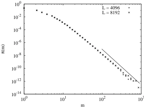
For the chipping model, CFR predicts that at ρ = ρc(w),
π(m)∼m−11/2, chipping model, d= 1. (21)
Monte Carlo simulations were done for lattices of size 4096 and 8192. The chipping rate w = 24.0. ρ was chosen to be ρ = ρc = 4.0. The results are shown in
Fig. 2. The data is consistent with the CFR predictions.
V. SUMMARY AND CONCLUSIONS
In this paper, we examined the consequences of a constant flux on two models where there were no obvi-ous conserved quantities and the dissipation and driving scales were not widely separated. The two models con-sidered were examples of systems undergoing nonequilib-rium phase transitions. CFR holds in the phases where
the probability distributions are power laws. The CFR prediction was borne out by numerical simulations. How-ever, an analytic approach is lacking. For this purpose,
10-14
10-12
10-10
10-8
10-6
10-4
10-2
100
100 101 102 103 104
π
(m)
m
[image:5.612.327.555.92.257.2]q = 0.3072 q = 1.0000
FIG. 1: The variation ofπ(m) withmis shown for differentq’s in the in-out model. The lower straight line has an exponent −3.5 and corresponds toq =qc(p). The upper straight line
has an exponent−2.0 and corresponds to the growing phase q≫qc(p).
10-14
10-12
10-10
10-8
10-6
10-4
10-2
100
100 101 102 103
π
(m)
m
L = 4096 L = 8192
FIG. 2: The variation ofπ(m) withmis shown for two differ-ent lattice sizes in the chipping model. ρ=ρc. The straight
line has an exponent−5.5.
one possibly needs to work with the effective field theories for these models.
[image:5.612.320.559.353.531.2][1] R. Drake, in Topics in Current Aerosol Research (part 2), Vol. 3, edited by G. Hidy and R. Brock (Pergamon Press, New York, 1972), p. 201.
[2] G. Huber, Physica A170, 463 (1991).
[3] S. N. Coppersmith, C. h Liu, S. Majumdar, O. Narayan, and T. A. Witten, Phys. Rev. E53, 4673 (1996). [4] C. h Liu, S. Nagel, D. A. Schecter, S. N. Coppersmith,
S. N. Majumdar, O. Narayan, and T. A. Witten, Science
269, 513 (1995).
[5] F. Leyvraz, Phys. Rep.383, 95 (2003).
[6] K. Kang and S. Redner, Phys. Rev. A30, 2833 (1984). [7] V. Privman, ed., Nonequilibrium Statistical Mechanics
in one dimensions (Cambridge University Press, Cam-bridge, 1997).
[8] S. Krishnamurthy, R. Rajesh, and O. Zaboronski, Phys. Rev. E66, 066118 (2002).
[9] R. Munasinghe, R. Rajesh, and O. Zaboronski, Phys. Rev. E73, 051103 (2006).
[10] R. Munasinghe, R. Rajesh, R. Tribe, and O. Zaboronski, Commun. Math. Phys268, 717 (2006).
[11] C. Connaughton, R. Rajesh, and O. Zaboronski, Physica
D222, 97 (2006).
[12] C. Connaughton, R. Rajesh, and O. Zaboronski, Phys. Rev. Lett98, 080601 (2007).
[13] A. N. Kolmogorov, Dokl. Akad. Nauk SSSR 32, 15 (1941), reprinted in Proc. Roy. Soc. Lond. A, 434, 15-17, (1991).
[14] U. Frisch,Turbulence: The Legacy of A. N. Kolmogorov (Cambridge University Press, Cambridge, 1995). [15] C. Connaughton, R. Rajesh, and O. Zaboronski, Phys.
Rev. Lett94, 194503 (2005).
[16] S. N. Majumdar, S. Krishnamurthy, and M. Barma, Phys. Rev. Lett81, 3691 (1998).
[17] S. N. Majumdar, S. Krishnamurthy, and M. Barma, Phys. Rev. E61, 6337 (2000).
[18] R. Rajesh, Phys. Rev. E69, 036128 (2004).
[19] S. N. Majumdar, S. Krishnamurthy, and M. Barma, J. Stat. Phys.99, 1 (2000).
[20] R. Rajesh and S. N. Majumdar, Phys. Rev. E63, 036114 (2001).