Modelling overdispersion with the normalized tempered stable distribution

University of Warwick institutional repository: http://go.warwick.ac.uk/wrap

This paper is made available online in accordance with

publisher policies. Please scroll down to view the document

itself. Please refer to the repository record for this item and our

policy information available from the repository home page for

further information.

To see the final version of this paper please visit the publisher’s website

.

Access to the published version may require a subscription.

Author(s): M Kolossiatis, JE Griffin and MFJ Steel

Article Title: Modelling overdispersion with the Normalized Tempered

Stable distribution

Year of publication: 2011

Link to published article: http://dx.doi.org/10.1016/j.csda.2011.01.016

Publisher statement: © Elsevier 2011. Kolossiatis, M. et al.

(2011). Modelling overdispersion with the Normalized

Modelling overdispersion with the Normalized

Tempered Stable distribution

M. Kolossiatis

_{, J. E. Griffin}

_{and M. F. J. Steel}

Abstract

This paper discusses a multivariate distribution which generalizes the Dirichlet distri-bution and demonstrates its usefulness for modelling overdispersion in count data. The distribution is constructed by normalizing a vector of independent Tempered Stable ran-dom variables. General formulae for all moments and cross-moments of the distribution are derived and they are found to have similar forms to those for the Dirichlet distribu-tion. The univariate version of the distribution can be used as a mixing distribution for the success probability of a Binomial distribution to define an alternative to the well-studied Beta-Binomial distribution. Examples of fitting this model to simulated and real data are presented.

Keywords: Mice Fetal Mortality; Normalized Random Measures; Overdispersion

1 Introduction

In many experiments we observe data as the number of observations in a sample with some property. The Binomial distribution is a natural model for this type of data. However, the data are often found to be overdispersed relative to that model. This is often explained and modelled through differences in the binomial success probability pfor different units. It is assumed thatxi successes (i.e.observations possessing a certain property) are observed fromn_i observations and thatx_i ∼Bi(n_i, p_i)wherep_i are drawn independent from some

∗_{Department of Statistics, University of Warwick, Coventry, CV4 7AL, U.K. and}† _{School of Mathematics,}

mixing distribution on(0,1). The Beta distribution is a natural choice since the likelihood has an analytic form. However, although analytically convenient, estimates will be biased if the data does not not support this assumption. Many other choices of mixing distribution have been studied including the Logistic-Normal-Binomial model (Williams, 1982) and the Probit-Normal-Binomial model (Ochi and Prentice, 1984). Altham (1978) and Kupper and Haseman (1978) propose a two-parameter distribution, the Correlated-Binomial, which allows for direct interpretation and assignment of the correlation between any two of the underlying Bernoulli observations of a Binomial random variable through one of its two parameters. Paul (1985) proposes a three-parameter generalization of the Beta-Binomial distribution, the Beta-Correlated Binomial distribution. There is also a modified version of the latter in Paul (1987). Brookset al(1997) use finite mixture distributions to provide a flexible specification. However, the introduction of a mixture distribution leads to more complicated inference and harder interpretation of parameters. Kuk (2004) suggests the

q-power distribution which models the joint success probabilities of all orders by a power family of completely monotone functions which extends the folded logistic class of George and Dowman (1995). Pang and Kuk (2005) define a shared response model by allowing each response to be independent of all others with probabilityπ or taking a valueZ with probability 1−π. Therefore more than one observation can take the common valueZ. They argue that this is more interpretable than the q-power distribution of Kuk (2004). Rodriguez-Aviet al(2007) use a Generalized Beta distribution as the mixing distribution.

In this paper, we consider an alternative specification for the distribution ofp_ifor which all cross-moments are available analytically. A random variableXon(0,1)can be defined by considering two independent positive random variablesV1andV2and taking

X = V1

V1+V2.

defined on the unit simplex. Normalized Tempered Stable distributions are indexed by a single additional parameter and can accommodate heavier tails and more skewness than would be possible for the Dirichlet distribution.

The paper is organized as follows: Section 2 discusses some background ideas: the Tempered Stable distribution and some distributions on the unit simplex. Section 3 de-scribes the Normalized Tempered Stable distribution and the form of its moments and cross-moments, Section 4 considers the use of this distribution as a mixing distribution in a Binomial mixture, Section 5 illustrates the use of the model for simulated and real data and compares its fit to other specifications and, finally, Section 6 concludes.

2 Background

This section describes the Tempered Stable distribution and some properties of the Dirichlet and Normalized Inverse-Gaussian distributions.

2.1 Tempered Stable distribution

The Tempered Stable (TS) distribution was introduced by Tweedie (1984).

Definition 1. A random variableXdefined onR+follows a Tempered Stable distribution with parametersκ,δandγ(0< κ <1,δ >0andγ >0) if its L´evy density is

u(x) =δ2κ κ Γ(1−κ)x

−1−κ_exp

½

−1 2γ

1/κ_x

¾ .

We will writeX∼TS(κ, δ, γ).

In general, the probability density function is not available analytically but can be ex-pressed through a series representation due to its relationship to the positive stable distribu-tion (see Feller, 1971)

f(x) =c

∞

X

k=1

(−1)(k−1)sin(kπκ)Γ(kκ+ 1)

k! 2

kκ+1_(xδ−1/κ₎(−kκ−1)_exp

½

−1 2γ

1/κ_x

¾

where c = ₂1_πδ−1/κexp{δγ}. The expectation ofX is 2κδγ(κ−1)/κ and its variance is

4κ(1−κ)δγ(κ−2)/κ_{. The moment generating function will be important for our derivations} and is given by

There are two important subclasses. A TS

³ κ, ν

κψ2κ, ψ2κ

´

will limit in probability asκ→0

to a Gamma distribution which has probability density function

f(x) = (ψ2/2)ν Γ(ν) x

ν−1_exp

½

−1 2ψ

2_x

¾

and the Inverse-Gaussian distribution arises when κ = 1₂ which has probability density function

f(x) = √δ

2π exp{δγ}x

−3/2_exp

½

−1 2(δ

2_x−1_+γ2_x)

¾

The Tempered Stable distribution is infinitely divisible and self-decomposable.

2.2 Dirichlet and Normalized Inverse-Gaussian distribution

The Dirichlet distribution is a commonly used distribution on the unit simplex.

Definition 2. Ann-dimensional random variableW = (W1, W2, . . . , Wn)is said to fol-low a Dirichlet distribution with parametersa1, a2, . . . , an+1 >0, denoted Dir(a1, a2, . . . , an+1), if its density is:

f(w) = Γ(a1+a2+· · ·+an+1) Γ(a₁)Γ(a₂)· · ·Γ(a_n+1)

n

Y

i=1

wai−1 i



₁₋

n

X

j=1

wj





an+1−1

,

wherew= (w1, . . . , wn)is such thatw1, . . . , wn≥0and0<

P_n

k=1wk<1.

The Dirichlet distribution can be generated through an obvious generalization of the normalization idea in Section 1 to a vector of (n+ 1)independent random variables for which thei-th entry has a Ga(ai,1)distribution. Its moments and cross-moments are easy to calculate and are as follows:

Proposition 1. LetW = (W1, . . . , Wn) ∼Dir(a1, a2, . . . , an+1) and letN1, N2, N ∈IN. DefiningS=Pn_i=1+1aiandµj =aj/S, we can state

1. E(WN

i ) = Γ(Γ(SS)Γ(+Na)Γ(i+Nai)) =

Q_N−1

k=0

³

ai+k S+k

´

, i= 1,2, . . . , n.

2. E(WN1

i WjN2) = Γ(Γ(SS)Γ(+Na1i++NN21)Γ()Γ(aai)Γ(j+Na2j)) =

Q_N1−1

k=0

³

ai+k S+k

´ Q_N2−1

l=0

³

aj+l S+N1+l

´

, i, j= 1,2, . . . , n, i6=j.

3. E(Wi) =µi

4. Var(Wi) = µi(1_S+1−µi) 5. Cov(W_i, W_j) =−µiµj

The Inverse-Gaussian distribution is an interesting sub-class of Tempered Stable distri-butions since its probability density function is available analytically. This is also true for the Normalized Inverse-Gaussian distribution (Lijoi et al, 2005) which is constructed by normalizing a vector of(n+ 1)independent random variables for which all entries have Inverse-Gaussian distributions. It is defined in the following way.

Definition 3. We say that ann-dimensional random variableW= (W1, W2, . . . , Wn) fol-lows a Normalised Inverse-Gaussian (N-IG) distribution with parametersν₁, ν₂, . . . , ν_n+1>

0, orW∼N-IG(ν1, ν2, . . . , νn+1),if

f(w) = exp

nP_n+1

i=1 νi

o Q_n+1

i=1 νi 2(n+1)/2−1_π(n+1)/2_A

n+1(w)(n+1)/4

K_−(n+1)/2³pAn+1(w)

´_Yn

i=1

w_i−3/2 

₁₋Xn

j=1

wj





−3/2

(2.2) wherew= (w1, . . . , wn)is such thatw1, . . . , wn≥0and0<

P_n−1

k=1wk<1,An+1(w) = n

X

i=1

ν2 i

wi +

ν_n2₊₁

1−Pm_j=1−1wj

andKis the modified Bessel function of the third type.

The expectation and variance of any componentWi, as well as the covariance structure of any two components,W_iandW_j of a N-IG-distributed random vectorW are given in Lijoiet al(2005):

Proposition 2. LetW = (W1, . . . , Wn)∼N-IG(ν1, ν2, . . . , νn+1). Then, 1. E(W_i) = νi

S =:µi, i= 1,2, . . . , n.

2. Var(Wi) =µi(1−µi)S2exp{S}Γ(−2, S), i= 1,2, . . . , n.

3. Cov(Wi, Wj) =−µiµjS2exp{S}Γ(−2, S), i, j= 1,2, . . . , n, i6=j. whereS =Pn_i=1+1νi and Γ(a, x) =

R_∞

x ta−1 exp{−t}dtis the incomplete Gamma func-tion.

3 Multivariate Normalized Tempered Stable

distri-bution

We define the Multivariate Normalized Tempered Stable (MNTS) distribution in the fol-lowing way.

TS(κ,νi

κ,1)and

Wi = _V Vi

1+V2+. . . Vn+1

thenW = (W₁, W₂, . . . , W_n)follows a Multivariate Normalized Tempered Stable distri-bution with parametersν andκwhich we denote as MNTS(ν1, ν2, . . . , νn+1;κ).

There are two special cases of this distribution. The Dirichlet distribution arises as

κ→0and the Normalized Inverse-Gaussian distribution arises ifκ= 1/2:

MNTS(ν1, ν2, . . . , νn+1;κ)−→κ→0Dir(ν1, ν2, . . . , νn+1)

in probability, and

MNTS(ν₁, ν₂, . . . , ν_n+1; 1/2)≡N-IG(2ν₁,2ν₂, . . . ,2ν_n+1).

All the moments and cross-moments of the n-dimensional MNTS distribution exist (since the distribution is defined on the n dimensional unit simplex) and the following theorem gives their analytic form.

Theorem 1. Suppose thatW= (W1, W2, . . . , Wn) ∼ MNTS(ν1, ν2, . . . , νn+1;κ)and let

N₁, N₂, N ∈IN. Then, definingS = n+1

X

i=1

ν_iandµ_i=ν_i/S, we have that

1. E¡WN i

¢

= N

X

l=1 N_X−1

j=0

bN(l, j) Γ

µ

l−j/κ,S κ

¶

2. E

³ WN1

i WjN2

´

= N1

X

l=1 N2

X

m=1

N1+XN2−1

t=0

cN1,N2(l, m, t) Γ

µ

l+m−t/κ,S κ

¶

where

bN(l, j) =

Ã

N−1

j !

(−1)N+j_(S/κ)j/κ _exp©S κ

ª

dN(κ, l)

Γ(N)l!κ µ

l i,

c_N1,N2(l, m, t) =

Ã

N1+N2−1

t

!

(−1)N1+N2+t_(S/κ)t/κ _exp©S

κ

ª

d_N1(κ, l)d_N2(κ, m) Γ(N1+N2)l!m!κ

µl_iµm_j ,

andd_N(κ, l) = l

X

i=1

à l i

!

(−1)i N_Y−1

c=0

(κi−c).

numbers, or generalized factorial coefficients,G(n, k, σ)(see, for example, Charalambides and Singh (1988) and Charalambides (2005)), through the simple formula

dN(κ, l) = (−1)Nl!G(N, l, k).

The expressions for the moments are weighted sums of incomplete Gamma functions which will have negative arguments. It was necessary to use a symbolic language, such as Mathematica, to accurately evaluate the cross-moments when N₁ andN₂ becomes large (over, say, 10). The corresponding code is freely available from:

http://www.warwick.ac.uk/go/msteel/steel homepage/software.

Corollary 1. IfW= (W1, W2, . . . , Wn)∼MNTS(ν1, ν2, . . . , νn+1;κ)then

E(Wi) =µi,

Var(Wi) = (1−κ)µi(1−µi)

"

1−

µ S κ

¶_1/κ

exp

½ S κ

¾

Γ

µ

1−1/κ,S κ

¶# ,

Cov(Wi, Wj) =µiµj

" κ+κS

κ −κexp ½

S κ

¾ µ S κ

¶_1/κ

Γ

µ

2−1/κ,S κ

¶

−1

#

=µ_iµ_j(1−κ)

"

exp

½ S κ

¾ µ S κ

¶_1/κ

Γ

µ

1−1/κ,S κ

¶

−1

# ,

and

Corr(W_i, W_j) =−

r µi 1−µi

µj 1−µj

.

The expectation of Wi and the correlation between Wi andWj do not depend on κ and have the same form associated with the Dirichlet and the Normalized Inverse-Gaussian distributions. The form of the variance generalizes the form for the Dirichlet and Normal-ized Inverse-Gaussian distributions since the variance ofW_i only depends on ν through

S =Pn_i=1νiand the meanµi =νi/S and we can write Var(Wi) =α(κ, S)µi(1−µi)for some functionα.

Applying the results of Theorem 1 to the special case of the Normalized Inverse-Gaussian distribution allows us to extend the results of Lijoi et al (2005) (as given in Proposition 2) to more general cross-moments:

Corollary 2. LetW= (W1, W2, . . . , Wn)∼N-IG(ν1, ν2, . . . , νn+1)then, forN, N1, N2∈

1. E£WN i

¤

= N

X

l=1 N_X−1

j=0

bN(l, j) Γ (l−2j,2S)

2. E

h WN1

i WjN2

i

= N1

X

l=1 N2

X

m=1

N1+XN2−1

t=0

cN1,N2(l, m, t) Γ (l+m−2t,2S)

where

bN(l, j) =

Ã

N−1

j !

(−1)N+j_S2j₂2j+1 _{exp{2S} d} N(l)

Γ(N)l! µ

l i,

cN1,N2(l, m, t) =

Ã

N1+N2−1

t

!

(−1)N1+N2+t_S2t₂2t+1 _exp{2S}d

N1(l)dN2(m)

Γ(N1+N2)l!m! µ

l iµmj ,

dN(l) = l

X

i=1

à l i

!

(−1)i N_Y−1

c=0

µ i

2−c

¶

,S= n+1

X

i=1

νi andµi = ν_Si.

In the calculation ofd_N(l)above, we only need to calculate the additive terms for odd values ofi, as the other terms will be 0.

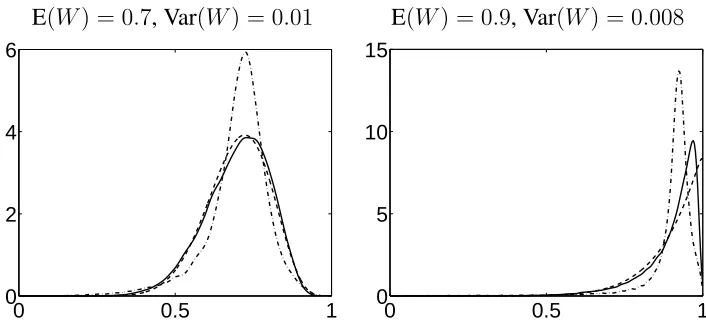
E(W) = 0.7, Var(W) = 0.01 E(W) = 0.9, Var(W) = 0.008

0 0.5 1

0 2 4 6

0 0.5 1

0 5 10 15

Figure 1: The densities of NTS distributions with the same mean and variance but different values ofκ. In each graph the values are: κ= 0(dashed line),κ= 0.5(solid line),κ= 0.9(dot-dashed line)

The univariate MNTS, which we term the Normalized Tempered Stable¡with parame-tersν1, ν2andκ, written NTS(ν1, ν2;κ)

¢

, is an important case and we study its properties in detail. Asκ → 0, the distribution tends to a Beta distribution with parametersν1 and

with heavier tails. The effect is more pronounced when the mean ofW is close to 1 (or 0). Figure 2 shows how the variance changes withκ (left), how the kurtosis changes withκ

(middle) and the relationship between the two, for a NTS(ν, ν;κ)distribution. Kurtosis is defined as the standardized fourth central moment:

Kurt(X) = E(X−E(X))

4

(Var(X))2 .

0 0.5 1

0 0.05 0.1 0.15 0.2 0.25

kappa

variance

0 0.5 1

0 2 4 6 8

kappa

kurtosis

0 0.05 0.1 0.15 0.2 0

2 4 6 8

variance

kurtosis

Figure 2:The Variance and kurtosis of NTS distribution with mean 0.5: (a) showsκversus the variance, (b) showsκversus the kurtosis and (c) shows variance versus kurtosis. In each graph: S = 0.1(solid line),S = 1(dashed line) andS = 10(dot-dashed line).

µ= 0.4 µ= 0.25 µ= 0.1

0 0.5 1

0.2 0.4 0.6 0.8 1

kappa

skewness

0 0.5 1

0.5 1 1.5 2 2.5 3

kappa

skewness

0 0.5 1

1 2 3 4 5 6

kappa

skewness

Figure 3:Skewness againstκfor various values of the mean for some NTS distributions. In each graph:

S = 0.1(solid line),S= 1(dashed line) andS = 10(dot-dashed line).

This graph shows that the variance decreases asκ increases. For other values of the first moment µ = ν1

ν1+ν2 the relationship between the variance andκis the same but the

From the shape of the graph of kurtosis plotted againstκ,one can see that asκincreases, the tails of the underlying TS distributions become heavier. There is a dramatic increase in kurtosis for values ofκgreater than 0.8. The shape of this graph is preserved for all values of the other parameters, ν1 andν2, and we note that the minimum kurtosis is not always achieved for the limiting case asκ → 0, although the value at this limit is very close to the overall minimum. Forµ→0, the value ofκthat gives the minimum value of kurtosis tends to 0.2, whereas for not very small values ofµ, the caseκ ' 0seems to provide the smallest kurtosis. There is also symmetry aroundµ= 1/2.The values of kurtosis increase as|µ−1/2|increases, whereas for large values ofκ, kurtosis decreases as S = ν1+ν2 increases, and for small values ofκkurtosis increases asS increases. In other words, the range of possible kurtosis values decreases withS.

In the right graph in Figure 2 we see the relationship between the variance and the kur-tosis forµ= 0.5.The shape again is the same for other values of the parametersν1andν2 and the graph is exactly the same forµand1−µ. The Beta distribution corresponds to the point at the left end of the graph (i.e. for smallest variance).

Let skewness of a distribution denote its standardized third central moment, i.e.

Skew(X) = E(X−E(X))3 (Var(X))3/2 .

Ifµ = 1/2the skewness is zero for all values ofκ. Figure 3 shows the skewness against

κ for various values of µandS. We only plot the skewness Skew(µ, S, κ) for µ < 0.5

since Skew(µ, S, κ) = −Skew(1−µ, S, κ)(which follows from the construction of the distribution). As the value ofµmoves away from 1/2, the value of skewness also increases in absolute terms. On the other hand, when the value ofS =ν1+ν2 increases, skewness decreases in absolute value. Finally, note that, as for kurtosis, the minimum skewness (maximum, forµ >1/2) is not achieved forκ '0, but (usually) for some value between 0 and 0.6.

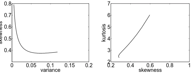
0 0.05 0.1 0.15 0.2 0.4

0.5 0.6 0.7 0.8

variance

skewness

0.22 0.4 0.6 0.8 1 3

4 5 6 7

skewness

kurtosis

Figure 4: Skewness against variance and kurtosis against skewness for some NTS distributions

the same endpoint corresponds to the Beta distribution, but to neither minimum skewness, nor to minimum kurtosis and the graph curls for both those quantities (rather than only for the skewness, as in Figure 4).

4 The NTS-Binomial distributions

In this section, we consider using the Normalized Tempered Stable distribution as a mixing distribution in a Binomial model. This can be written as

Xi∼Bi(ni, Pi), Pi ∼NTS(ν1, ν2;κ).

The NTS(ν1, ν2;κ)mixing distribution represents the heterogeneity in the probability of success across the different observed groups. The response can be written as the sum ofn

Bernoulli random variables,Xi =

P_ni

j=1Zi,jwhereZi,1, Zi,2, . . . , Zi,niare i.i.d. Bernoulli with success probabilityPi. The intra-group correlation is defined as Corr(Zi,k, Zi,j)which in our model has the form

ρ= (1−κ)

"

1−

µ S κ

¶_1/κ

exp

½ S κ

¾

Γ

µ

1−1/κ,S κ

¶#

. (4.3)

whereS =ν1+ν2. The variance ofXi can be written as

Var(Xi) =n2iVar(Pi) +niE[Pi(1−Pi)]

The formulae for the moments derived in Theorem 1 can now be used to derive the likelihood for an observed samplex= (x1, x2, . . . , xn):

f(x) =

Z ₁

0 · · ·

Z ₁

0

f(x|p1, . . . , pN)f(p1, . . . , pN)dp1. . . dpN

= N

Y

i=1

Z ₁

0

f(xi|pi)f(pi)dpi

= N

Y

i=1

à ni

xi

!

Epi

¡ pxi

i (1−pi)ni−xi

¢

where the expectation is given by the result in Theorem 1.

5 Examples

5.1 Simulated data

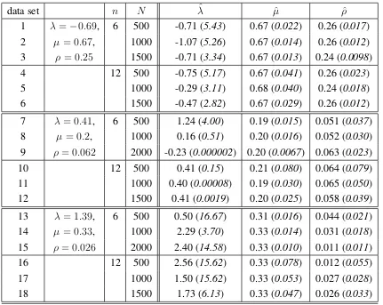
This simulation study considers the effectiveness of Maximum Likelihood estimation for the NTS-Binomial and compares its results with the Beta-Binomial model. We created 18 data sets by simulating from the NTS-Binomial model with different parameter values. The model is parameterized by(λ, µ, ρ)whereλ= logκ−log(1−κ),µ=ν1/(ν1+ν2)and

ρis the intra-group correlation defined in (4.3). The number of observations for each unit

n_i is set equal to a common value n. The NTS-Binomial and the Beta-Binomial models were fitted to each data set. The Beta-Binomial is parameterized asµ=ν1/(ν1+ν2)and

data set n N λˆ µˆ ρˆ

1 λ=−0.69, 6 500 -0.71 (5.43) 0.67 (0.022) 0.26 (0.017) 2 µ= 0.67, 1000 -1.07 (5.26) 0.67 (0.014) 0.26 (0.012) 3 ρ= 0.25 1500 -0.71 (3.34) 0.67 (0.013) 0.24 (0.0098) 4 12 500 -0.75 (5.17) 0.67 (0.041) 0.26 (0.023) 5 1000 -0.29 (3.11) 0.68 (0.040) 0.24 (0.018) 6 1500 -0.47 (2.82) 0.67 (0.029) 0.26 (0.012) 7 λ= 0.41, 6 500 1.24 (4.00) 0.19 (0.015) 0.051 (0.037) 8 µ= 0.2, 1000 0.16 (0.51) 0.20 (0.016) 0.052 (0.030) 9 ρ= 0.062 2000 -0.23 (0.000002) 0.20 (0.0067) 0.063 (0.023) 10 12 500 0.41 (0.15) 0.21 (0.080) 0.064 (0.079) 11 1000 0.40 (0.00008) 0.19 (0.030) 0.065 (0.050) 12 1500 0.41 (0.0019) 0.20 (0.025) 0.058 (0.039) 13 λ= 1.39, 6 500 0.50 (16.67) 0.31 (0.016) 0.044 (0.021) 14 µ= 0.33, 1000 2.29 (3.70) 0.33 (0.014) 0.031 (0.018) 15 ρ= 0.026 2000 2.40 (14.58) 0.33 (0.010) 0.011 (0.011) 16 12 500 2.56 (15.62) 0.33 (0.078) 0.012 (0.055) 17 1000 1.50 (15.62) 0.33 (0.053) 0.027 (0.028) 18 1500 1.73 (6.13) 0.33 (0.047) 0.026 (0.033)

Table 1:Maximum likelihood estimates forλ, µ, andρfor the NTS-Binomial model with the simulated data sets.

the NTS-Biomial model compared with the Beta-Binomial model (results not shown). The

(a) (b)

0 0.5 1

0 1 2 3

0 0.5 1

0 2 4 6 8

Figure 5: Density of the mixing distribution for the NTS-Binomial (solid line) and Beta-Binomial (dashed line) models evaluated at the maximum likelihood estimates for: a) λ = −0.69, µ = 0.67,

True value NTS-Binomial Beta-Binomial

n N Skew Kurt Skew Kurt Skew Kurt

λ=−0.69, 6 500 -0.617 2.39 -0.634 2.38 -0.572 2.38

µ= 0.67, 1000 -0.620 2.43 -0.577 2.51

ρ= 0.25 1500 -0.622 2.41 -0.608 2.46 12 500 -0.643 2.39 -0.591 2.41 1000 -0.692 2.52 -0.587 2.45 1500 -0.643 2.41 -0.567 2.41

λ= 0.41, 6 500 1.07 4.26 1.470 6.04 0.521 3.15

µ= 0.2, 1000 0.922 3.89 0.721 3.38

ρ= 0.062 2000 0.916 3.79 0.707 3.38 12 500 1.040 4.14 0.681 3.32 1000 1.070 4.31 0.676 3.38 1500 1.050 4.21 0.678 3.35

λ= 1.39, 6 500 0.571 3.52 0.516 3.08 0.180 2.96

µ= 0.33, 1000 1.070 6.02 0.249 2.92

ρ= 0.026 2000 0.803 5.19 0.143 2.97 12 500 0.959 6.10 0.152 2.97 1000 0.625 3.71 0.229 2.93 1500 0.698 4.04 0.224 2.92

Table 2:The skewness and kurtosis evaluated at the maximum likelihood estimate for the NTS-Binomial and Beta-Binomial models with the simulated data sets.

5.2 Mice fetal mortality data

Brookset al(1997) analyze six data sets of fetal mortality in mouse litters. The data sets are: E1, E2, HS1, HS2, HS3 and AVSS. E1 and E2 were created by pooling smaller data sets used by James and Smith (1982), HS1, HS2 and HS3 were introduced by Haseman and Soares (1976) and the AVSS data set was first described by Aeschbacheret al (1977). In each data set, the data were more dispersed than under a Binomial distribution. Brookset al(1997) show that finite mixture models fit the data better than the standard Beta-Binomial model in all data sets except AVSS. Here, we fit the NTS-Binomial and its special case whenκ= 1/2, the N-IG-Binomial model, as alternatives. Several other models have been applied to these data including the shared response model of Pang and Kuk (2005) and theq-power distribution of Kuk (2004). We use the data with the correction described in Garrenet al(2001).

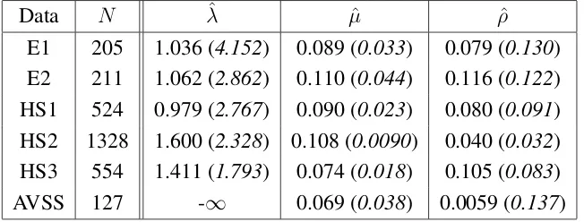
Data N λˆ µˆ ρˆ

E1 205 1.036 (4.152) 0.089 (0.033) 0.079 (0.130) E2 211 1.062 (2.862) 0.110 (0.044) 0.116 (0.122) HS1 524 0.979 (2.767) 0.090 (0.023) 0.080 (0.091) HS2 1328 1.600 (2.328) 0.108 (0.0090) 0.040 (0.032) HS3 554 1.411 (1.793) 0.074 (0.018) 0.105 (0.083) AVSS 127 -∞ 0.069 (0.038) 0.0059 (0.137)

Table 3: Maximum likelihood estimates with standard errors for the parameters in NTS-Binomial model for the six mice fetal mortality data sets.

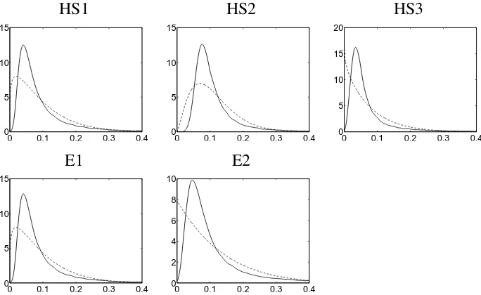
Table 3 shows the maximum likelihood estimates of the parameters of the NTS-Binomial models with their related asymptotic standard errors (shown in parentheses). In all data sets except AVSS the estimate ofλis substantially different fromλ=−∞(which corresponds to the Beta-Binomial case). In the other data setsλis estimated to be between 0.979 and 1.6 which correspond toκvalues between 0.74 and 0.83. This suggests that the estimated mixing distributions are substantially different from a Beta distribution. In fact the tails of the distribution are much heavier than those defined by a Beta distribution with the same mean and variance. The estimated mixing distributions are shown in Figure 6 with the mixing distribution for the Beta-Binomial distribution (the AVSS data set is not included since the estimates for NTS-Binomial and Beta-Binomial models imply the same mixing distribution).

HS1 HS2 HS3

0 0.1 0.2 0.3 0.4 0

5 10 15

0 0.1 0.2 0.3 0.4 0

5 10 15

0 0.1 0.2 0.3 0.4 0

5 10 15 20

E1 E2

0 0.1 0.2 0.3 0.4 0

5 10 15

0 0.1 0.2 0.3 0.4 0

2 4 6 8 10

Figure 6: Density of the mixing distribution for the NTS-Binomial (solid line) and Beta-Binomial (dashed line) models evaluated at the maximum likelihood estimates for the mice fetal mortality data set

NTS-Binomial Beta-Binomial Skew Kurt Skew Kurt E1 2.75 13.26 1.41 2.42 E2 2.66 11.99 1.42 2.25 HS1 2.67 12.62 1.41 2.42 HS2 2.66 13.57 1.00 1.21 HS3 3.89 22.93 1.65 3.46

Table 4: Estimates of the skewness and kurtosis of the mixing distributions for the Beta-Binomial and NTS-Binomial distributions

third and especially fourth moments are much larger for the NTS-Binomial model which confirms the interpretation ofκgiven in Section 3.

Criterion (AIC) and the Bayesian Information Criterion (BIC) are used as measures of fit. IfLis the maximum likelihood value,nis the data size andkis the number of parameters, the AIC=−2 logL+ 2kand the BIC=−2 logL+klogn.

Model E1 E2 AVSS HS1 HS2 HS3

Beta-Binomial +8.3 +6.0 341.9 +9.3 +43.9 +32.8 NTS-Binomial +4.8 +1.1 +2.0 +1.2 +24.1 +3.4 N-IG-Binomial +5.1 +0.6 +0.5 +3.1 +38.9 +18.8 B-B/B mixture +3.5 +0.4 +3.8 1550.3 3274.7 1373.9

2-d binom. mixture +1.7 +0.6 +1.9 +20.6 +20.1 +4.6 3-d binom. mixture +5.1 +1.9 +5.7 +1.1 +4.1 +1.8 Best binom. mixture +5.1 +1.9 +9.7 +4.5 +1.7 +5.5 Shared response 563.1 687.8 +6.1 +20.3 +42.5 +8.9

q-power +6.6 +8.4 +8.0 +6.5 +2.1 +0.5 Correlated-Binomial +26.2 +36.7 +1.2 +57.0 +67.3 +94.5 B-C-B +7.8 +1.3 +2.0 +8.4 +35.7 +24.0 Table 5: AIC values for the competing models for each data set. The smallest value for each data set is shown in bold and other AIC values are shown as differences from that minimum.

Results for each data set are given in Table 5 (for AIC) and Table 6 (for BIC). The best model has the smallest value of the information criterion. In both tables, the smallest value of AIC/BIC for each of the data sets are given in bold and the values for the other models are given as differences from the best model. In the tables, B-B/B mixture is the Beta-Binomial/Binomial mixture (i.e. a mixture consisting of a Beta-Binomial part and a Binomial part), 2-d/3-d correspond to mixtures of two or three Binomials respectively, B-C-B is the Beta-Correlated-Binomial model, and N-IG is the normalised Inverse-Gaussian distribution. Finally, the best Binomial mixture is a mixture of Binomials with the number of components unknown. The number of components to be fitted is derived using the program C.A.MAN, using directional derivative methods (see Bohninget al(1992)). We also found that the log likelihood value given by Pang and Kuk (2005) for E1 was not consistent with their estimates. Their value seems to correspond to the data set given by Brookset al(1997) rather than the corrected version given by Garrenet al(2001).

Model E1 E2 AVSS HS1 HS2 HS3 Beta-Binomial +8.3 +6.0 347.6 +6.2 +41.9 +32.3 NTS-Binomial +8.1 +4.5 +4.9 +2.4 +27.2 +7.2 N-IG-Binomial +5.1 +0.6 +0.5 1561.9 +36.8 +18.3 B-B/B mixture +10.2 +4.6 +9.5 +5.4 +8.3 +8.2 2-d binom. mixture +5.0 +4.0 +4.8 +21.7 +23.2 +8.4 3-d binom. mixture +15.1 +12.0 +14.2 +10.8 +17.5 +14.3 Best binom. mixture +15.1 +12.0 +23.9 +22.7 +25.6 +26.6 Shared response 569.7 694.5 +6.1 +17.2 +40.4 +8.4

q-power +6.6 +7.9 +9.0 +3.4 3287.2 1383.0

Correlated-Binomial +26.2 +36.7 +1.2 +53.9 +65.2 +94.0 B-C-B +11.1 +4.6 +4.9 +9.6 +38.8 +27.8 Table 6:BIC values for the competing models for each data set. The smallest value for each data set are shown in bold and other BIC values are shown as differences from that minimum.

AVSS data, the Beta-Binomial model is the best model with the N-IG-Binomial coming a close second. Considering the HS1-HS3 data sets, the differences between the criterion values of the different models are larger than in the other data sets, due to the much larger data size. For HS1, the N-IG-Binomial model is actually the best in terms of the BIC, whereas the B-B/B mixture performs best in terms of the AIC. The value of AIC for the N-IG-Binomial model and the value of BIC for the B-B/B mixture are, as one would expect, close to the smallest values. The NTS-Binomial model is the second best in terms of BIC and third (but also very close to the second) in terms of AIC. The best model for the HS2 and HS3 data is the B-B/B mixture in terms of AIC and theq-power model in terms of BIC. For HS3, the NTS-Binomial is second best in terms of BIC and fourth in terms of AIC.

6 Discussion

model, which is the Binomial model mixed with an univariate MNTS distribution on the success probability. In our examples the NTS-Binomial outperforms the Beta-Binomial and is competitive with other previously proposed models.

References

Abramowitz, M. and Stegun, I. A. (1964): “Handbook of mathematical functions with for-mulas, graphs, and mathematical tables, Volume 55 of National Bureau of Standards Applied Mathematics Series,”

Aeschbacher, H. U., Vuataz, L., Sotek, J., and Stalder, R. (1977): “The use of the Beta-Binomial distribution in dominant-lethal testing for weak mutagenic activity (Part 1),”Mutation Research, 44, 369-390.

Altham, P. M. E. (1978): “Two generalizations of the Binomial distribution,” Applied Statistics, 27, 162-167.

Billingsley, P. (1995): “Probability and measure,” John Wiley & Sons: New York. Bohning, D., Schlattmann, P. and Lindsay, B. (1992): “Computer-Assisted Analysis of

Mixtures (C.A.MAN): Statistical Algorithms,”Biometrics, 48, 283-303.

Brix, A. (1999): “Generalized Gamma measures and shot-noise Cox processes,”Advances in Applied Probability, 31, 929-953.

Brooks, S. P. (2001): “On Bayesian analyses and finite mixtures for proportions,” Statis-tics and Computing, 11, 179-190.

Brooks, S. P., Morgan, B. J. T., Ridout, M. S. and Pack, S. E. (1997): “Finite Mixture Models for Proportions,”Biometrics, 53, 1097-1115.

Charalambides, Ch. A. (2005): “Combinatorial methods in discrete distributions” John Wiley & Sons: Hoboken, New Jersey.

Charalambides, Ch. A. and Singh, J. (1988): “A review of the Stirling numbers, their gen-eralizations and statistical applications,” Communications in Statistics-Theory and Methods, 17, 2533-2595.

Feller, W. (1971): “An introduction to probability theory and it applications,” John Wiley & Sons: New York.

George, E. O. and Bowman, D. (1995): “A full likelihood procedure for analysing ex-changeable binary data,”Biometrics, 51, 512-523.

Gradshteyn, I. S. and Ryzhik, I. M. (1994): “Table of integrals, series and products,” Academic Press: Boston.

Haseman, J.K . and Soares, E. R. (1976): “The distribution of fetal death in control mice and its implications on statistical tests for dominant lethal effects,” Mutation Research, 41, 272-288.

Hougaard, P. (1986): “Survival models for heterogeneous populations derived from stable distributions,”Biometrika, 73, 387-396.

James, D. A. and Smith, D. M. (1982): “Analysis of results from a collaborative study of the dominant lethal assay,”Mutation Research, 97, 303-314

James, L. F., Lijoi, A. and Pr¨unster, I. (2006): “Conjugacy as a distinctive feature of the Dirichlet process,”Scandinavian Journal of Statistics, 33, 105-120.

Johnson, W. P. (2002): “The curious history of Fa´a di Bruno’s formula,”American Math-metical Monthly, 109, 217-234.

Jorgensen, B. (1987): “Exponential dispersion models (with discussion),”Journal of the Royal Statistical Society B, 49, 127-162.

Kuk, A. Y. C. (2004): “A litter-based approach to risk assessment in developmental tox-icity studies via a power family of completely monotone functions,”Journal of the Royal Statistical Society. Series C., 53, 369-386.

Kupper, L. L. and Haseman, J. K. (1978): “The use of a correlated Binomial model for the analysis of certain toxicological experiments,”Biometrics, 35, 281-293.

Lijoi, A., Mena, R. H. and Pr¨unster, I. (2005): “Hierarchical mixture modeling with nor-malized inverse-Gaussian priors,” Journal of the American Statistical Association, 100, 1278-1291.

Ochi, Y. and Prentice, R. L. (1984): “Likelihood inference in a correlated probit regression models,”Biometrika, 71, 531-543.

Palmer, K. J., Ridout, M. S. and Morgan, B. J. T. (2008a): “Modelling cell generation times using the Tempered Stable distribution,”Journal of the Royal Statistical Society Series C, 57, 379-397.

Palmer, K. J., Ridout, M. S. and Morgan, B. J. T (2008b): R functions for the Tempered Stable distribution (R code). Available from

Pang, Z. and Kuk, A. Y. C. (2005): “A shared response model for clustered binary data in developmental toxicity studies,”Biometrics, 61, 1076-1084.

Paul, S. R. (1985): “A three-parameter generalisation of the Binomial distribution,” Com-munications in Statistics Theory and Methods, 14(6), 1497-1506.

Paul, S. R. (1987): “On the Beta-Correlated Binomial (BCB) distribution in a three pa-rameter generalization of the Binomial distribution,” Communications in Statistics Theory and Methods, 16(5), 1473-1478.

Tweedie, M. (1984): “An index which distinguishes between some important exponential families,” inStatistics: Applications and New Directions: Proceedings of the Indian statistical Institute Golden Jubilee International Conference, Eds: J. Ghosh and J. Roy, 579-604.

Williams, D. A. (1982): “Extra-Binomial variation in logistic linear models,”Journal of the Royal Statistical Society C, 31, 144-148.

A Proofs

A.1 Proof of Theorem 1, part 1

We exploit the representation of the Normalized Tempered Stable distribution through Tem-pered Stable random variables. If W ∼ MNTS(ν1, ν2, . . . , νn+1;κ) then we can write

Wi = V_Vi whereV =

P_n+1

j=1 Vj,V1, V2, . . . , Vn+1 are independent andVj ∼TS(κ, νj

κ,1). Then, we have:

E£W_iN¤=E

· VN i VN ¸ =E · VN i Γ(N)

Z _∞

0

uN−1exp{−uV}du ¸

= 1

Γ(N)

Z _∞

0

uN−1 Y

j6=i

E[exp{−uVj}] E

£

V_iNexp{−uVi}

¤

du (A.4)

= (−1)N Γ(N)

Z _∞

0

uN−1 Y

j6=i

E[exp{−uVj}] E

· ∂N

∂uN exp{−uVi}

¸ du

= (−1)N Γ(N)

Z _∞

0

uN−1 Y

j6=i

E[exp{−uVj}] ∂ N

∂uN E[exp{−uVi}] du (A.5)

= (−1) N Γ(N) exp

½ S κ

¾ Z _∞

0

uN−1 exp

 

− X

j6=i

ν_j

κ(1 + 2u)

κ

 

 ∂N

∂uN exp

n

−νi

κ(1 + 2u)

κo

| {z }

(1)

du

(A.6)

(A.3) is an application of the Fubini Theorem and (A.4) is an application of Theorem (16.8) in Billingsley (1995). Finally, for (A.5) we used the know form for the moment generating function of the Tempered Stable distribution.

The difficulty is to calculate (1), i.e. theN-th derivative of the functionexp©−νi

κ(1 + 2u)κ

ª

. This is possible using Meyer’s formula, which is a variation of Faa di Bruno’s formula (see, for example, Johnsonet al(2002)): iffandgare functions with sufficient derivatives then

∂N

∂uN(g◦f)(x) =

∂N

∂uN [g(f(u))] = N

X

l=0

g(l)(f(u))

l!

½ ∂N

∂hN [f(u+h)−f(u)] l ¯ ¯ ¯ ¯ h=0 ¾

In this case,g(x) = exp{x}andf(x) =−νi

κ(1 + 2x)κ. We first consider:

[f(x+h)−f(x)]l= νil

κl[(1 + 2x)

and the derivative can be seen to be

∂N

∂hN [f(x+h)−f(x)] l₌ νil

κl l X i=0 Ã l i !

(−1)i(1 + 2x)κ(l−i)

· ∂N

∂hN(1 + 2x+ 2h) κi

¸

The derivative can be expressed as

∂N

∂hN(1 + 2x+ 2h)κi= 2Nκi(κi−1)· · ·(κi−N+ 1)(1 + 2x+ 2h)κi−N So, ath= 0, we get:

∂N

∂hN[f(x+h)−f(x)] l ¯ ¯ ¯ ¯ h=0

= 2Nνil

κl l X i=1 Ã l i !

(−1)i(1 + 2x)κ(l−i) N_Y−1

c=0

(κi−c)(1 + 2x+ 2h)κi−N

¯ ¯ ¯ ¯ ¯ h=0

= 2Nν l i κl l X i=1 Ã l i !

(−1)i(1 + 2x)κl−N N_Y−1

c=0

(κi−c)

By plugging the above in Meyer’s formula, and noting that g(k)_{(f(x)) = g(f(x)) =}

exp©−νi

κ(1 + 2x)κ

ª

, we can see that

∂N

∂uN exp

n

−νi

κ(1 + 2u)

κo_{= 2}N N

X

l=1

exp©−νi

κ(1 + 2u)κ

ª l! νl i κl l X j=1 Ã l j !

(−1)j(1 + 2u)κl−N N_Y−1

c=0

(κj−c)

= 2N N

X

l=1

exp©−νi

κ(1 + 2u)κ

ª

l!

ν_il

κl(1 + 2u)κl−NdN(κ, l) (A.7) where

d_N(κ, l) = l X j=1 Ã l j !

(−1)j N_Y−1

c=0

(κj−c) = l X j=1 Ã l j !

(−1)j Γ(κj+ 1) Γ(κj−N + 1)

It is now straightforward to verify that

E¡W_iN¢= (−1)

N₂N_exp©S κ

ª

Γ(N)

N

X

l=1 νl

i

κldN(κ, l)

l!

Z _∞

0

uN−1 exp

½

−S

κ(1 + 2u)

κ

¾

(1+2u)κl−Ndu.

The integral in the last expression can be simplified using the substitutiony = (1 + 2u)κ and the Binomial theorem:

Z _∞

0

uN−1 exp

½

−S

κ(1 + 2u)

κ

¾

(1+2u)κl−Ndu= 1 2N_κSl

κl N_X−1

j=0

à N −1

j !

(−1)jSj/κ

κj/κΓ

µ

l−j/κ,S κ

¶

and therefore

E¡W_iN¢= N

X

l=1 N_X−1

j=0

Ã

N−1

j !

(−1)N+jexp©S_κªdN(κ, l) Γ(N)l!κ

µ S κ

¶_j/κ³ νi

S ´_l

Γ

µ

l−j/κ,S κ

A.2 Proof of Theorem 1, part 2

For the cross-moments of the MNTS distribution, we have:

E

h WN1

i WjN2

i

=E

" VN1

i VjN2

VN

#

, whereN =N1+N2

=E

" VN1

i VjN2 Γ(N)

Z _∞

0

uN−1 exp{−uV}du #

=(−1)N Γ(N)

Z _∞

0

uN−1 E

· ∂N1

∂uN1 exp{−uVi}

¸

E

· ∂N2

∂uN2 exp{−uVj}

¸ Y

t6=i,j

E[exp{−uV_t}]du

=(−1) N Γ(N)

Z _∞

0

uN−1 ∂

N1

∂uN1E[exp{−uVi}]

∂N2

∂uN2E[exp{−uVj}]

Y

t6=i,j

E£exp©−uVt

ª¤ du

=(−1) N Γ(N) exp

½ S κ

¾ Z _∞

0

uN−1 ∂

N1

∂uN1

³

exp

n

−νi

κ(1 + 2u)

κo´

× ∂ N2

∂uN2

³

exp

n

−νj

κ(1 + 2u)

κo´_exp

 

− X

t6=i,j

νt

κ(1 + 2u)

κ

 

du

Using the result for theN−th derivative of the functionexp©−νi

κ(1 + 2u)κ

ª

in (A.6), we find:

E

³ WN1

i WjN2

´

= (−1)N Γ(N) exp

½ S κ ¾ 2N N1 X l=1 N2 X m=1

dN1(κ, l)dN2(κ, m)

l!m!

νl i

κl

ν_jm

κmIl,m∗ (κ) where

I_l,m∗ (κ) =

Z _∞

0

uN−1 exp

½

−S

κ(1 + 2u)

κ

¾

(1 + 2u)κ(l+m)−N du.

Using the same substitution as above,y= (1+2u)κ_{, inI}∗

l,m(κ),together with the Binomial theorem, we find:

E

³ WN1

i WjN2

´ = N1 X l=1 N2 X m=1

N1+XN2−1

t=0

cN1,N2(l, m, t)Γ

µ

l+m−t/κ,S κ

¶

(A.8)

where

cN1,N2(l, m, t) =

Ã

N1+N2−1

t

!

(−1)N1+N2+t_(S/κ)t/κ _exp©S

κ

ª

dN1(κ, l)dN2(κ, m)

Γ(N1+N2)l!m!κ µ

l

iµmj . ¤

A.3 Proof of Corollary 1

For the first moment we have:

b1(1,0) =

Ã

0 0

!

(−1)1exp©S_κªν_i1

Γ(1)1!κ1+0/κ_S1−0/κ(−κ), andd1(κ,1) =−κ⇒b1(1,0) = exp

The result follows from noting that Γ¡1−0/κ,S_κ¢ = Γ¡1,S_κ¢ = RS∞

κ exp{−t}dt =

exp©−S_κª.

The second moment is

E£W_i2¤=−(1−κ)µi(1−µi)S 1/κ

κ1/κ exp

½ S κ ¾ Γ µ

1−1/κ,S κ

¶

+µi(1−κ+µiκ)

sinced2(κ,1) =

Ã

1 1

!

(−1)1_{(κ−0)(κ−1) =κ(1−κ)andd}

2(κ,2) = 2κ2, which im-plies thatb2(1,0) = (1−κ) exp

©_S

κ

ª

µi,b2(1,1) =−(1−κ) exp

©_S

κ

ª µiS

1/κ

κ1/κ,b2(2,0) =

κexp©S_ꪵ2

i andb2(2,1) = −κexp

©_S κ ª µ2 iS 1/κ

κ1/κ. The result follows from noting that

Γ¡1−0/κ,S κ

¢

= exp©−S κ

ª

andΓ¡2−0/κ,S κ

¢

= exp©−S κ

ª ¡

1 +S κ

¢

.

In order to calculate the covariance we only have to calculatec1,1(1,1,0)andc1,1(1,1,1). Noting thatd1(κ,1) =−κit follows that

c_1,1(1,1,0) =

Ã

1 0

!

(−1)2_exp©S κ

ª

(−κ)2ν1i κ1

ν1

j κ Γ(2)1!1!κS1+1−0/κ

κ1+1−0/κ

= exp

½ S κ

¾ κ νiνj

S2 = exp

½ S κ

¾ κµ_iµ_j

c1,1(1,1,1) =

Ã

1 1

!

(−1)3_exp©S κ

ª ν1

iνj1 Γ(2)1!1!κS_κ1+11+1−−11/κ/κ

=−exp

½ S κ

¾ κS1/κ

κ1/κ

νiνj

S2 =−exp

½ S κ

¾

κµiµjS 1/κ

κ1/κ

The fact thatΓ¡1 + 1−0/κ,S_κ¢= Γ¡2,S_κ¢= exp©−S_κª ¡1 +S_κ¢implies that

E[WiWj] =κµiµj

"

1 +S

κ −exp ½ S κ ¾ µ S κ

¶_1/κ

Γ

µ

2−1/κ,S κ

¶# .

Subtracting E(Wi)E(Wj) from the above, we derive the formula for the covariance of