Implementation and Analysis of Real time Object Tracking on the Starburst MPSoC

December 16, 2015

MASTER THESIS

IMPLEMENTATION AND

ANALYSIS OF REAL-TIME

OBJECT TRACKING ON THE

STARBURST MPSOC

VIKTORIO S. EL HAKIM

Electrical Engineering, Mathematics and Computer Science (EEMCS) Computer Architecture for Embedded Systems (CAES)

EXAMINATION COMMITTEE: Prof. dr. ir. M.J.G. Bekooij Ir. J. (Hans) Scholten G. Kuiper, M.Sc.

Documentnumber

University of Twente

MASTER THESIS

Implementation and

Analysis of Real-Time

Object Tracking on the

Starburst MPSoC

Author:

Student number:

Committee:

V.S.e. Hakim

s1415778

Prof. dr. ir. M.J.G. Bekooij

Ir. J. (Hans) Scholten

G. Kuiper, M.Sc.

Computer Architecture for Embedded Systems

(CAES), Department of EEMCS, University of Twente,

Abstract

Computer vision has experienced many advances over the recent years. As such, it started to rapidly find its way into many commercial and industrial applications, with the disciplines of visual object detection and tracking being most prominent. A good example of computer vision being applied in practice, is the social network and website Facebook, where advanced object detection algorithms are utilized to detect and recognize people and in particular – their faces. One of the main reasons for the rapid expansion of computer vision in practice, is the ever emerging new computing platforms, such as the cloud service, capable to handle the complex mathematics involved in analyzing and extracting information from images.

Despite its advances however, computer vision is still in its early stages of establishing a solid foothold in the world of embedded systems. Specifically, systems which are subjected to real-time constraints, with restricted compu-tational resources, are struggling the most. Thus the usage of modern visual object detection and tracking algorithms in safety critical embedded systems is still more or less restricted. Fortunately, this is starting to change with newly developed embedded computer architectures, which employ application specific hardware to perform the task of computer vision more efficiently.

In this thesis, two state-of-the-art computer vision algorithms in the form of HOG-SVM detection and Particle filter tracking, are explored and evaluated on a real-time embedded MPSoC, calledStarburst. Eventually, it can be shown that these two seemingly “difficult” algorithms, not only can satisfy certain real-time constraints, but also achieve a high throughput on an embedded system such as Starburst. To accomplish this, the thesis contributes with a powerful real-time hardware architecture of the HOG object detector, and a software based multiple processor object tracking framework, based on the Particle filter.

Acknowledgements

First and foremost, I would like to thank Prof. Marco Bekooij, for giving me the opportunity to work under his supervision, on this interesting and challenging project. Additionally, I highly appreciate the amount of feedback and motiva-tion he gave me, throughout the course of my master thesis assignment, as well as sparking my interest in real-time multiprocessor development.

Next, I would like to thank all of my colleges in the Pervasive Systems (PS) and CAES groups. Specifically I would like to thank Alex and Vignesh from the PS group, for the amount of time spent together, drinking coffee and discussing various scientific topics, and the additional feedback and suggestions provided about my thesis. Another special thank you goes to O˘guz, who kept me company during my research, and helped me on various occasions with the Xilinx toolchain.

List of Abbreviations

ADC Analog-to-Digital Converter

API Application Program Interface

AR Auto-Regressive

ARMA Auto-Regressive Moving Average

ASIC Application-Specific Integrated Circuit

BRAM Block Random Access Memory

CAES Computer Architectures for Embedded Systems

CDF Cumulative Distribution Function

CLB Configurable Logic Block

CMOS Complementary Metal–Oxide–Semiconductor

CORDIC COordinate Rotation DIgital Computer

CPU Central Processing Unit

CSDF Cyclo-static Data-flow

DMA Direct Memory Access

DSP Digital Signal Processing

EKF Extended Kalman Filter

ES Embedded System

ET Execution Time

FPGA Field-Programmable Gate Array

FPS Frames Per Second

GPS Global Positioning System

GPU Graphics Processing Unit

HMM Hidden Markov Model

HOG Histogram of Oriented Gradients

INRIA Institute for Research in Computer Science and Automation

LIDAR LIght Detection And Ranging

MB Microblaze

MC Monte Carlo

MPSoC MultiProcessor System-on-Chip

MSB Most Significant Bits

PCA Principle Component Analysis

PDF Probability Density Function

PDP Dot Product

PF Particle Filter

PPF Parallel Particle Filter

RGB Red Green Blue

RMS Root Mean Square

RMSE Root Mean Squared Error

RNG Random Number Generator

RT Real-Time

RTOS Real-Time Operating System

RTS Real-Time System

SDF Synchronous Data-flow

SIR Sequential Importance Resampling

SMC Sequential Monte Carlo

TDM Time Division Multiplexing

TP Throughput

UAV Unmanned Aerial Vehicle

VGA Video Graphics Array

List of Figures

2.1 Division hierarchy from image to window, to blocks and finally -cells. . . 9

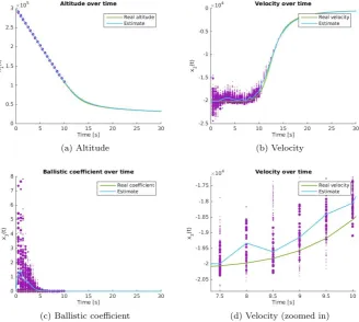
3.1 Sketch of the system; the blue box represents the distance sensor, while the orange sphere represents the falling object . . . 24

3.2 System simulation plots; the purple dots represent the particles set for each state variable before resampling, with their respective sizes proportional to the weights . . . 24

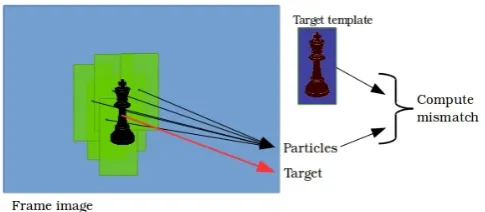
3.3 Graphical illustration of the particle weighting process for the Visual PF . . . 28

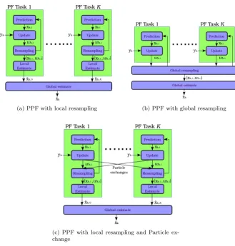
3.4 Three prominent PPF implementation schemes. The edges rep-resent deterministic data transfer channels. . . 34

4.1 Block diagram of a typical, processor onlyStarburst configuration 40

4.2 Structural diagram of the HOG-SVM detector. . . 42

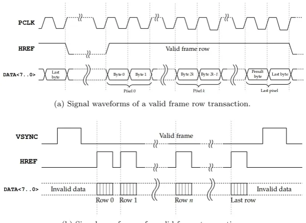
4.3 Signal descriptions and waveforms of a typical CMOS image sen-sor’s parallel data interface . . . 43

4.4 Signal descriptions and waveforms of a typical CMOS image sen-sor’s parallel data interface . . . 44

4.5 Block diagram of the image gradient filter . . . 45

4.6 Hardware implementation modules of fully unrolled CORDIC al-gorithm in vectoring mode. . . 47

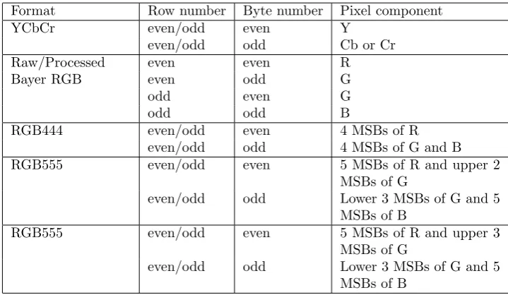
4.7 Illustration of a “sliding” 2-by-2 block of 8-by-8 pixel cells, along the widthW of the gradient magnitude and orientation images. The red pixel refers to gm[k] andgo[k], while the green pixels refer togm[k−W l] andgo[k−W l]; 0< l≤15 . . . 48

4.8 A situation, where the block is split across the image due to buffering. . . 49

4.9 A buffering topology for the gradient magnitude and quantized orientation streams. . . 49

4.10 Bin accumulation hardware for one 8×8 cellj, with histogram length ofL= 8.. . . 50

4.11 Adder tree with selective input. The dashed lines indicate poten-tial pipe-lining. . . 50

4.12 Block diagram of the HOG block vector normalizer. The dotted lines indicate the linear interpolation block for the division. . . . 51

4.15 Sharing of a block (indicated in red) by four overlapping detection windows at the top-left corner of the image frame. The brighter the color, the more overlap introduced. . . 54

4.16 Parallel Particle filter task graph and communication topology . 55

4.17 Different exchange strategies. Here, the blue block represents the old local set of particles, while the green blocks - the sets of particles, received from neighboring processors. . . 57

4.18 Particle exchanging by passing particles around the ring topol-ogy. The purple boxes represent the top D particles of task

τi, i= 1, ..., P, while the green boxes – exchanged particles from a neighbor. . . 58

5.1 Input image at different down-scale factors, with the detection output images superimposed on top. . . 63

5.2 RMSE of each state variable. . . 67

5.3 RMSE of each state variable vs. number of particles per task amount. . . 68

5.4 RMSE of each state variable vs. number of exchanged particles per task amount and number of exchanges. . . 69

5.5 RMSE and WCET vs. number of particles per processor amount. 70

5.6 Execution time of the exchange step, vs . . . 71

5.7 WCET and TP vs. number of processors . . . 71

5.8 Typical measured execution time of the exchange step. . . 72

5.9 WCET of a PPF iteration vs. exchanged particle and neighbor amount. . . 73

5.10 Some example frames of the PF object tracking process and the reference frame image. . . 74

5.11 The real and estimatedxandytrajectories of the orange, over a 80 of iterations. . . 75

6.1 Parallel Particle filter task graph and communication topology . 79

6.2 HOG detector RT CSDF model. . . 80

6.3 Parallel Particle filter SDF model. . . 81

List of Tables

3.1 Parameters values for falling body PF tracking example . . . 25

4.1 Pixel byte interpretation per format . . . 44

5.1 Optimal configuration parameters of the HOG detector, given a 320x240 frame image resolution . . . 64

Contents

1 Introduction 1

1.1 Problem definition . . . 2

1.2 Contributions . . . 4

1.3 Thesis outline . . . 4

2 The HOG-SVM object detector 7 2.1 HOG features . . . 8

2.1.1 Gradient calculation . . . 8

2.1.2 Window and cell formation . . . 9

2.1.3 Block formation and histogram normalization . . . 10

2.1.4 Feature vector . . . 11

2.1.5 Classification using linear SVMs . . . 11

2.2 Algorithm analysis and bottlenecks . . . 11

2.2.1 Gradient calculation . . . 11

2.2.2 Window extraction and cell formation . . . 12

2.2.3 Cell HOG binning . . . 12

2.2.4 Block formation and normalization . . . 13

2.2.5 SVM dot product. . . 13

2.2.6 Summary . . . 14

2.3 Design considerations and trade-offs . . . 14

2.3.1 Cell and block size . . . 14

2.3.2 Choice of histogram length . . . 15

2.3.3 Block normalization . . . 15

3 Tracking using Particle Filters 17 3.1 Algorithm definition . . . 18

3.1.1 Bayesian state estimation . . . 18

3.1.2 Sequential Importance Sampling . . . 19

3.1.3 The Resampling Step . . . 21

3.1.4 SIR example . . . 22

3.2 Visual Tracking . . . 25

3.2.1 Motion Model. . . 26

3.2.2 Measurement Model . . . 28

3.3 Computational complexity and bottlenecks . . . 30

3.3.1 Prediction step analysis . . . 31

3.3.2 Update step analysis . . . 32

3.3.3 Resampling step . . . 32

3.4.1 Parallel Software Implementation. . . 33

3.4.2 Hardware acceleration . . . 35

3.5 Design considerations . . . 36

3.5.1 Number of Particles . . . 36

3.5.2 Resampling Algorithm . . . 37

3.5.3 Motion model. . . 37

3.5.4 Observation model and features. . . 37

4 System implementation 39 4.1 Starburst MPSoC. . . 39

4.2 HOG-SVM detector . . . 41

4.2.1 Overview . . . 41

4.2.2 CMOS Camera peripheral . . . 42

4.2.3 Gradient filter module . . . 45

4.2.4 CORDIC module . . . 45

4.2.5 Block extraction module . . . 47

4.2.6 Normalization module . . . 51

4.2.7 SVM classification module. . . 52

4.3 Multicore Parallel PF . . . 54

4.3.1 PPF topology. . . 54

4.3.2 Particle exchange . . . 57

5 Analysis and experimental results 61 5.1 HOG-SVM detector evaluation . . . 61

5.1.1 Test setup and parameters. . . 61

5.1.2 Simulation results . . . 62

5.1.3 Optimal parameters . . . 62

5.1.4 Hardware resource usage. . . 64

5.2 PPF evaluation . . . 64

5.2.1 Test setup and parameters. . . 64

5.2.2 PC evaluation results . . . 65

5.2.3 Starburst evaluation results . . . 66

5.2.4 Visual tracking performance. . . 71

6 Conclusions 77 6.1 HOG detector. . . 77

6.2 Parallel particle filters . . . 78

6.3 Future Work . . . 78

6.3.1 HOG detector. . . 79

6.3.2 Parallel Particle Filter . . . 79

6.3.3 Real-time Analysis . . . 80

Appendices 83 A Function definitions 85 A.1 atan2 function . . . 85

A.2 mod function . . . 85

Chapter 1

Introduction

Computer vision is an emerging discipline in computer science and electronic engineering, which strives at giving computers and machines the ability to per-ceive the environment in a similar way as humans do with the eyes. It covers a wide range of topics, such as machine learning, image and signal processing, video processing and control engineering. This invaluable ability allows ma-chines to perform more intelligent tasks and thus provide a better service to their human operators. Computer vision has easily found its way into commer-cial applications, such as medical imaging, image search, medical robotics and others.

Nowadays, two of the major topics in computer vision are object recogni-tion and tracking. Objects and features being extracted are used directly in the control systems of robots, smart vehicles, UAV’s, smart traffic monitoring, etc, allowing intelligent control and decision making. Up until recently, the main means of object detection has mostly relied on other technologies such as LIDAR, since the incoming data is much easier to process in real-time. With the recent discoveries of new feature extractors and robust tracking algorithms, modern computer vision systems have shown perfomance comparable to that of traditional object detection systems, if not even better. One of the main rea-sons is the fact that vision also provides information about the appearance of the object(s) and the surroundings. This is particularly attractive in the area of personal assistance devices, where LIDAR systems for example are not appro-priate due to their size. Nevertheless it is not uncommon to see combinations of traditional and vision based sensors, such as Google’s self driving car project.

To complement this trend even further, recent decline in costs of CMOS im-age sensors made computer vision even more accessible to the world of embedded systems. Cheap camera modules can provide mobile platforms with a constant stream of rich visual information about the environment, at a relatively small cost and scale. This is particularly important in the area of portable electronics. To satisfy the growing need of long lasting and comfortable to carry electronics, portables rely heavily on embedded systems, due to their small factor, low-power usage and low-cost.

of the underlying algorithms. These embedded systems simply cannot guaran-tee that the needed information arrives on time and is indeed reliable. To make it more clear it is the vast amount of incoming raw data needed to be processed, that makes it challenging for an embedded system to extract useful information in real-time.

Standard personal computers equipped with powerful processors and GPU’s can easily handle modern computer vision algorithms. But due to the power and cost restrictions, it is not feasible to install conventional computers on mobile platforms. Instead, a common technique is to perform vision on a remote computer or cluster, and receive control commands from there. But for mobile safety critical applications, the latency introduced is unacceptable.

Nowadays, there has been a huge surge of systems on chip incorporating multiple processing cores and hardware acceleration, dedicated for a specific task. The synergy between software and hardware allows the system to be both flexible and keep up with high throughput constraints. Indeed the intermediate usage of hardware, allows embedded systems to easily achieve throughputs, comparable to a pure software implementation on a high-end PC.

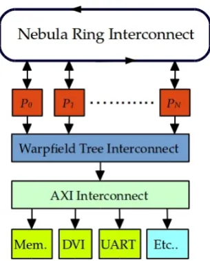
One such system is theStarburstMPSoC, actively developed at the chair of Computer Architectures for Embedded Systems (CAES), University of Twente, and the main development platform of this thesis. At the moment, the system is deployed on a Xilinx ML605 development board, featuring a high-capacity Virtex-6 FPGA, allowing plenty of room to study and evaluate embedded com-puter vision. It consists of multiple ring interconnected processors, which exe-cute a RTOS known as Helix. Multi-processor software can be easily analyzed using real-time tools and eventually deployed on the cores, guaranteeing fair and deterministic behavior. Unfortunately it still lacks the hardware capabilities to handle computer vision effectively.

Therefore the focus of this thesis is to implement and evaluate a state-of-the-art object recognition and a tracking system, both in hardware and software, on theStarburstMPSoC. This technical report summarizes and describes the whole design process and decisions involved during the development of the system. In this chapter, the reader is introduced to the research problem. Section one defines the problem in more detail and raises the appropriate research objectives. Section two states the contributions made by this thesis. Finally section three describes the outline of this report.

1.1

Problem definition

need to work at a much higher frequency, resulting in higher power consumption. Although one can opt to incorporate a big amount of low-frequency cores in the system instead, this scheme brings a lot of other problems to the table, such as memory contention. To ensure fair sharing of resources between cores, a system usually assigns time slices to each of them for using a particular resource. This introduces be a big bottleneck, making parallel execution of computer vision algorithms that rely on big amounts of memory very difficult. These and other similar restrictions are very common to embedded devices, which try to maintain a low-power profile and small form factor. A big advantage of software implementations however are their flexibility and reconfigurability.

In contrast, a pure hardware implementation is not limited by the amount of processing available, but the amount of resources. In ASIC terms, this refers to the area on a chip and the chip process. In FPGA terms, hardware resources take form of BRAM, DSP slices and general purpose CLBs. Hardware gives a designer the power to more easily take advantage of inherent parallelism in an algorithm. Thus it is quite common that hardware implementations often exhibit per-pixel execution for each of the steps in an object detection and tracking processing pipeline. This results in drastic reduction of memory usage, as the need to store most of the data is eliminated, and lower power usage since the processing is done at a relatively low frequency. A big disadvantage however of purely hardware based solutions is the limited flexibility and configuration options. This is problematic because of the dynamic nature of most computer vision systems. The ability to change the parameters on the fly is very important in safety applications.

Taking both advantages and disadvantages of hardware and software into consideration, this thesis puts forward the following objectives:

1. Extend theStarburstMPSoC with hardware and software, that can handle generic video input from standard CMOS camera sensors.

2. Research and evaluate the state-of-the-art HOG-SVM object detection and Particle Filter tracking algorithms –

(a) Determine the trade-offs between efficiency and robustness, of differ-ent implemdiffer-entations;

(b) Identify their respective bottlenecks, and how to optimally mitigate their effect on an implementation, both in hardware and software; (c) Evaluate an optimal solution in software.

3. Realize a robust, visual object detection and tracking system based on

Starburst, capable of achieving real-time performance with high through-put –

(a) Develop an efficient and capable hardware design of the HOG-SVM object detection framework;

(b) Implement a Particle Filter based object tracker in software, comple-mented with appropriate hardware accelerators;

(c) Integrate the detector and tracker subsystems, while maintaining good balance between software and hardware.

(a) Find and reduce any combinatorial paths in the hardware design; (b) Estimate the resource usage in software and optimize appropriately.

(c) Make use of real-time analysis tools to determine the limits of the system and identify more bottlenecks

5. Test the system in a real-world setup. The research question put forward is as follows:

Is the Starburst architecture suitable for computer vision algorithms? More precisely is it suitable for modern object detection and tracking algorithms that must satisfy real-time constraints? If not, then what should be incorporated in the architecture to make it suitable?

1.2

Contributions

There are four major contributions of this research. First, this thesis contributes with a unique and highly-configurable hardware implementation of the famous HOG feature person detector[1]. The algorithm has been presented during the 2013 Embedded Vision Summit, generating a lot of interest among computer vision practitioners and embedded system engineers. Its simplicity and effectiveness for the problem of general object class detection, and in particular -people, is the main motivation for its consideration in this thesis.

Second, a parallel particle filter based object tracking framework is designed to run on multiple cores, utilizing the Helix RTOS on Starburst. Since the PPF is implemented purely in software, it can be easily adapted for any track-ing process. Additionally, it takes full advantage of the underlytrack-ing Starburst

architecture to achieve maximum potential.

Third, evaluation and analysis results are provided, to determine the tem-poral and functional performance of each algorithm. From a RTS perspective, this analysis gives insight into the reliability of the total system. From an ES perspective - insight about the efficiency.

Finally, a direct contribution is made for theStarburstMPSoC. By extending its hardware capabilities to handle embedded vision applications, this thesis provides means to further study algorithms in the area of computer vision on the MPSoC, and evaluate their real-time performance.

What this thesis does NOT contribute to is new ideas and algorithms in the field of computer vision. The focus is purely on evaluation and implementation of modern feature extraction and tracking techniques, therefore it heavily relies on available and proven research.

1.3

Thesis outline

So far, the first chapter introduced the reader to the topic of this thesis and the associated research questions. This section describes how the report is organized and a description of each chapter.

its components. It is then concluded with a small analysis and design consider-ations, which are used further in the actual hardware implementation.

Chapter three deals with object tracking. In particular, it focuses on the particle filter and its effective use in visual object tracking. First, important notions which are part of the PF framework, such as the SMC simulation, are introduced. Afterwards the notion of parallel particle filters is discussed. The focus is then directed on the usage of PFs for the problem of visual object tracking and how image features are used for particle weight calculation. Finally, the chapter is concluded again with a discussion on design considerations and particular bottlenecks associated with the particle filter, which will come in play later on.

Chapter four describes the implementation of the system. First an overview of the whole system is provided, while subsequent sections describe each part. Starting with hardware based feature extraction, to software implementation of tracking.

Chapter five presents the results. First, results related to the HOG detec-tor are presented, such as hardware resources usage, simulation and parameter optimization.

Chapter 2

The HOG-SVM object

detector

HOG features have proven on many occasions to be very effective for the task of object description and detection. Especially when combined with a linear SVM classifier. They were first discovered and used by researchers Dalal and Triggs, and described in their prominent paper[1], which has been considered by many as a state-of-the-art work. Subsequently, it has spawned many applications and extenstions, with one of the most prominent examples being the discriminative parts-based object detector by Felzenszwalb et. al.[2,3]. A comprehensive study on the performance of HOG-SVM based detectors and reasoning behind their success can be found in [4].

HOG stands for “Histograms of Oriented Gradients” and as the name sug-gests, the descriptor consists of image gradient orientation histograms, extracted from image patches representing the object(s) of interest. Another descriptor based on a similar principle and also sharing a big amount of success in the field of object detection is Lowe’s SIFT[5]. The work by Lowe certainly motivated the creation of the HOG descriptor. However it is important to note that SIFT was designed with a different purpose in mind. It is used to describe rotation and scaled invariant regions, local to the object(s) of interest. This usually results into a lot of descriptors extracted offline from an object template, which are subsequently stored in a data-base for matching purposes. It is therefore very suitable for image or video frame matching, but not for object classification. In contrast, HOG features are typically extracted from a dense grid of “cells”, as part of a detection window. Hence they describe an object in its entirety and shape, and are not restricted to the appearance of the object. This makes them very suitable and effective for classification using SVMs. One major drawback is their inability to detect objects in different poses, thus prompting the use of multi-class SVMs, as in [3].

2.1

HOG features

Histograms of Oriented Gradients are high-level features, which make use of the image gradient to describe an image patch. The constructed feature vector is subsequently used to detect objects of interest using a classifier. Feature vectors are also used to train the classifier. A general sequence of image processing steps are undertaken to extract the HOG features, summarized as follows:

1. Compute the image gradient approximations using horizontal and vertical kernels [−1,0,1] and [−1,0,1]T _{respectively.}

2. Compute the gradient magnitude and orientation images. This step trans-forms the gradient from rectangular to polar form.

3. Given a fixed window size, select a location on the gradient magnitude and orientation images, and extract an image patch within the window boundaries.

4. The patch is then divided into cells of equal size, along the width and height of the window. It is recommended to choose window size, such that it is a perfect multiple of the cell size.

5. For each cell, a histogram of some length L is constructed, where each bin represents quantized gradient orientations. Each gradient pixel from the cell casts a vote proportional to the magnitude into the bin where the pixel’s orientation belongs.

6. To improve the descriptor’s invariance to brightness and intensity fluc-tuations, cells are grouped into overlapping blocks. For each block, the cells’ histograms are concatenated together to form a vector, which is then normalized. There is a wide choice of normalization functions.

7. Once all block vectors are generated, they are all concatenated to form the final descriptor.

8. The descriptor can now be fed into an SVM classifier, to determine whether the object of interest is present or not in the current window. Multiple descriptors are used to train the classifier.

9. Detections across all scales and positions are interpolated, to find the exact position and scale, based on the score of the SVM decision function.

2.1.1

Gradient calculation

It is important to note that contrary to popular belief, applying a Gaussian filter or similar to the image before computing the gradient, is actually not recom-mended, as found by Dalal and Triggs. They also found that any other kernel used to compute the gradients, like the Sobel filter, also reduces performance. Conveniently, this makes the task of gradient calculation quite easy, especially in hardware. Generally, the gradients are computed from an image’s intensity, but it is possible to use all three RGB channels for more discriminative detection. The gradient is computed using the following equation:

∇I(x, y) =

Ix(x, y) Iy(x, y) ≈

I(x+ 1, y)−I(x−1, y) I(x, y+ 1)−I(x, y−1)

whereI(x, y) is the image intensity at discrete coordinatesxandy. The gradient is then converted into polar form with the relations1

k∇I(x, y)k₂=

q

Ix2+Iy2 (2.2)

θ∇I(x,y)= atan2(Iy, Ix) ∈ (−π, π] (2.3)

2.1.2

Window and cell formation

After the gradient is computed and transformed into polar form, the resulting magnitude and orientation images are “scanned” using a sliding window for detection purposes. For training purposes, specific window patches containing the object of interest are extracted by hand from training images. The window size used for people detection is usually 64×128. The window is then divided into cells of some size. Dalal and Triggs found that the algorithm performs best with cell sizes of 6×6 pixels and 8×8 pixels. Due to the obvious mathematical properties however, a 8×8 cell is used throughout this thesis. The hiearchy of the divisions (including blocks) is demonstrated in Fig. 2.1.

Figure 2.1: Division hierarchy from image to window, to blocks and finally -cells.

Next, gradient orientation histograms can be computed for each cell. The choice of histogram length is important and it depends on the orientation range. It is shown, that 9 and 18 bins is the optimal amount to achieve good detection rate for unsigned and signed orientation respectively. Lower amounts tend to reduce the performance. Furthermore the use of unsigned gradient orientation, i.e. |atan2(Iy, Ix)| ∈ [0, π], leads to better detection rate. Typically, the bin index is computed by quantizing the histogram orientation, given the histogram length and the orientation range, but this can cause magnitude votes to be casted in the “furthest” bin, even though they are much closer to its left or right neighbor (depending on the quantization method). To reduce this ambiguity, the

vote casted by each magnitude pixel can be split between the two neighboring bins, proportionally to the differences of the corresponding orientation and the orientations represented by the bins. Nevertheless the histogram in its simplest form is defined by the equation

H(i) =X x,y

M(x, y, i) 0≤i < L;i, L∈N (2.4)

where

M(x, y, i) =

(

k∇I(x, y)k₂, ifh(atan2(Iy, Ix)) =i

0, otherwise

andhis a quantization function, typically represented as

h(x) = _x 2π + 1 2

×L, (2.5)

if the orientation is signed and

h(x) =jx π

k

×L (2.6)

otherwise.

2.1.3

Block formation and histogram normalization

Once histograms are computed, cells are grouped into overlapping blocks, such that each block shares the majority with its neighbors, but excludes at least one row or column of cells. The order of cells doesn’t matter, as long as it is the same during training and detection. This process not only introduces redundancy, but also allows the histograms to be normalized around a whole region, reducing the influence of intensity and brightness fluctuations significantly and therefore - improving the detection rate. Dalal and Triggs found block sizes of 2×2 and 3×3 cells to be the most optimal with respect to cell size, with the latter giving the best results. In this thesis, a block size of 2×2 is used.

During the grouping process, histograms of the corresponding cells are con-catenated together to form a row vector of features. The vector is then normal-ized using one of the following relations

L2-norm: x = _q v

kvk2₂+e2

(2.7)

L1-norm: x = v

kvk₁+e (2.8)

L1-sqrt: x =

r _v

kvk₁+e (2.9)

wherev is the block histogram vector andx is the resulting normalized vector. The constante should be small, but its exact value is not specified.

2.1.4

Feature vector

Finally, the normalized block histogram vectors are all concatenated to form the feature vector. This vector has a very high dimensionality. For instance, a 64×128 window, divided by 8×8 cells, results into 105 2×2 blocks. If the histogram length per cellL= 8, the dimensionality of the feature vector is 3,360. This is perhaps the biggest bottleneck of the algorithm, resulting in a lot of memory usage and complex mathematical operations. Of course for smaller objects(which don’t require a big detection window) the dimensionality would reduce, but not substantially.

2.1.5

Classification using linear SVMs

Once the feature vector is acquired by the steps described above, it can be directly fed into a linear SVM classifier. The linear SVM is a binary decision classifier, governed by the score function

y(x) =w·x+b (2.10)

wherex is the input feature vector, andw andb are a vector of weights and a bias constant respectively, estimated during the training process. The decision function used to determine whether a windowk contains the object of interest or not is defined as

f(xk) =

(

1, ify(xk)>0

0, otherwise (2.11)

2.2

Algorithm analysis and bottlenecks

By now, the reader should be able to understand the steps undertaken to per-form object detection, by means of HOG features and a linear SVM classifier. However it hasn’t yet been clarified, what is the efficiency of the method, with respect to different implementations and parameters. This section tries to sum-marize various bottlenecks of the algorithm and the expected resource usage and computational complexity on standard sequential machines. It does so with hopes to give a clear picture of the inner workings of the method and simplify the design process further in this thesis.

2.2.1

Gradient calculation

The gradient component images are computed using kernels [−1,0,1] and [−1,0,1]T_. This is perhaps the least computationally intensive method, involving only two subtractions per pixel. If the convolution is implemented to directly process the image in a raster scan-like fashion, it requires only two memory locations for the horizontal kernel and two line buffers for the vertical. Conveniently, these kernels give the best detection results, as pointed out by Dalal and Triggs.

using an iterative method, with Newton-Raphson being the most prominent. This method can either be implemented in software or in hardware, as part of a floating-point accelerator, such as the ARM NEON™[6] engine or Intel®’s SSE[7]. Regardless, each of these operations require a lot of instruction cycles per pixel, especially if no floating-point accelerator is present on the underlying architecture. The exact number is largely architecture and method dependent. This bottleneck becomes a big problem on embedded architectures and there-fore cannot be remedied, without sacrificing accuracy, such as using fixed-point arithmetic instead of floating point. In some methods, ROM memory is also used for look-up tables, such as linear interpolation. However, this bottleneck affects only the throughput of the algorithm and not its potential real-time performance, as most approximation methods are deterministic.

2.2.2

Window extraction and cell formation

During the detection process, a patch of the image encompassed by a window is extracted at each possible position(defined by the top-left pixel coordinate of the patch), where the window can fit. This act of “sliding” the window and extracting the pixels is followed by forming cells. The whole process involves a lot of memory reads and writes, thus resulting in yet another bottleneck.

Why is it a bottleneck? A typical implementation of the extraction process would result into (W−Ww+ 1)×(H−Hw+ 1) windows being extracted, where

W and Ww are the image and window widths respectively, and H and Hw -the heights. Then per each window, a total of W ×Hw pixels are accessed from the frame buffers, storing the image gradient magnitude and orientation, for cell formation and histogram binning. This involves a lot of read and write operations and can significantly reduce the through-put of the detection system. Also the amount of memory used is unacceptable for embedded operations. The effect of data transportation is not evident in high-end processing systems, but becomes in embedded systems. Caching and/or sharing the data also introduces non-determinism in the system - highly undesirable for real-time operation. Keep in mind however, that one does not need to store the whole image in the frame buffers, but only enough to hold a window.

There isn’t a direct solution to reduce the memory usage and data trans-portation. The only solution is to exploit how the raw pixel data arrives and compute the histograms as pixels arrive from the input video device, after being processed by the steps earlier. This solution will further be explored in this thesis, when discussing the hardware implementation.

2.2.3

Cell HOG binning

Histogram binning involves accumulation of gradient magnitude pixel values into bins, based on the orientation value at the same pixel locations. Besides the memory bottleneck introduced earlier, there are others during the summation and quantization processes themselves.

That is why, the orientation should first be quantized, before feeding each pixel to the orientation frame buffer. This avoids the need to compute the bin index during the binning process.

Second, a total amount of 64 additions are required to fill each bin. If interpolation is used, the computational complexity is even bigger. However keeping track of the histograms, by adding only “newly” arrived pixels and throwing away “old” pixels in a raster-scan fashion can significantly improve bin accumulation in that regard. To elaborate further, suppose that A is a matrix of gradient magnitude pixels representing a cell, as part of the frame buffer. Assuming that pixels arrive along the width of an image, the histogram can be updated by subtracting the values from the last column ofAand adding the column of pixels next to the cell from the frame buffer. A is updated accordingly as well, since new data is shifted in the frame buffer. This results into 17 additions and one subtraction per cell - a great improvement! This method is also explored later in this thesis.

Another very powerful approach is to use the so called integral histogram[9], based on integral images. An example, where HOG-like features are extracted using this approach for PF based tracking is described by Yang et al[10]. Instead of performing accumulation “on-the-fly”, integral images are first computed for each bin. Computing the histograms for each cell then amounts to two additions and one subtraction per bin/integral image. In total however, the amount of additions stays relatively the same as the previously described method. However it makes histogram extraction quite easy on a sequential machine. The obvious disadvantage is the additional frame buffers required for each bin, added to the fact that this method doesn’t map well in hardware.

2.2.4

Block formation and normalization

To form blocks, one has to first compute the cell histograms. Subsequently, histograms are concatenated together to form a block vector and eventually normalized using of the norms, defined by Eq. 2.7,2.8 or 2.9. The act of con-catenation itself involves copying the histograms of the cells involved into a new memory locations and then normalizing.

The most prominent computation hurdle is the amount divisions involved during normalization. It can be reduced to one, by first computing the reciprocal of the norm and then multiplying each of the vector components. The amount of multiplications can be also reduced to one, by exploiting the dot product in the SVM score function. This is discussed later. As for the actual norm function, the complexity depends on the design choice. The L2-norm and L1-sqrt are the most computationally expensive, but the miss rate of the detector is significantly reduced. L1-norm increases the miss rate slightly, compared to the other norms, but it is computationally light since it involves only additions. One must thus accept these trade-offs and decide if accuracy is important, compared to algorithmic efficiency.

2.2.5

SVM dot product

number of multiplications is governed by the following relation, assuming an 8×8 cell size and window sizeWw×Hw:

M =

_H

w 8 −1

·

_W

w 8 −1

·p2·L mod(Hw,8) = 0 ∧ mod(Ww,8) = 0 (2.12) whereM is the total multiplications amount,p- block width and height in cells,

L - histogram length and mod(a, b) is the modulus function of two integers1_.

The number of additions is the same, including the SVM bias constant. This step can only be accelerated by splitting the dot product into smaller dot products of block vectors and performing multiplications in parallel. The results of these products are gradually accumulated, until the final block of the window is “filled” in. A simple comparison operation is then needed to deter-mine whether an object is detected or not. Afterwards, the memory location which holds the sum can be reused for a new window. Most of these small dot products can be calculated efficiently on a processor with DSP capabilities, possibly reaching single clock cycle execution. This is the exact approach used by Hahnle et al.[11] and the implementation described by this report.

2.2.6

Summary

The HOG-SVM detector is a very complex and computationally heavy algo-rithm. Memory storage, data transportation and non-linearity of operations are the most dominant sources of bottlenecks. Yet a lot of its features can be exploited, such as parameter tweaking and the way data is acquired, to increase the efficiency of the algorithm. A lot of the non-linear operations can be ap-proximated and efficiently implemented in hardware to achieve single clock cycle performance, which is the major advantage of hardware vs. software implemen-tations. Most memory locations can be reused for newer data, with the old one safely thrown away.

2.3

Design considerations and trade-offs

This section summarizes some parameter considerations of the algorithm and their associated trade-offs. It provides a small discussion for each step, to explain the reasoning behind these design decisions. Since the associated design choices affected the out-come of the final implementation, it is beneficial in case that reader is interested in the though process behind those decisions.

2.3.1

Cell and block size

In [1], the authors experimented with various cell and block sizes and found that any combination of 8×8 or 6×6 cells with 2×2 or 3×3 blocks give the most optimal results. A cell size of 6 and block size of 3 give the best result. Cells sizes of 6 and 8 share the same performance for block size of 2.

The soon to be discussed hardware implementation however uses a cell size of 8 and block size of 2, since both integers are a power of two. This allows easy multiplication and division by means of simple shifts, which becomes useful

in counting processes later on. Additionally as it will be seen later, this allows design of “perfect” binary adder trees, which is more than welcome in the design. All of this will come at the cost of slight performance drop.

2.3.2

Choice of histogram length

In their research, Dalal and Triggs found that increasing the length of the gra-dient orientation histogram increases performance significantly, by minimizing miss rate. However, they also show that using unsigned orientation as opposed to signed, cuts the length by a factor of two, while giving similar results. This means for example, that choosing a length of 18 for the full range of 0°to 360°, gives equivalent results for a length of 9.

In this thesis, a histogram length of 8 is used. Again the main reason is the fact that 8 is a power of two and therefore maps very well in hardware. Combined with a block size of 2, the resulting block vector will have a length of 32. Any multiplications or divisions by 8 or 32 can be substituted with a simple shift operation. Signed orientation is used to accommodate the small length. As seen in the results section in[1], this configuration gives close to optimal performance.

2.3.3

Block normalization

Normalization is a very important step during the HOG extraction process and therefore cannot be skipped. It is shown that any normalization function significantly improves the detection accuracy. However with greater accuracy, comes higher computational cost which translates into more hardware resources when implementing the detector on an FPGA.

Chapter 3

Tracking using Particle

Filters

The Particle Filter(PF) is a general name for a class of approximate Bayesian state estimation techniques, which rely on successive Monte Carlo simulations to solve the filtering problem. One of its earliest versions is the Sequential Importance Resampling(SIR) filter, or “the bootstrap algorithm” as introduced by Gordon et al.[12]. As demonstrated in the paper, the Particle Filter proves to be an extremely effective state estimation technique for general non-linear problems, as it greatly outperforms EKF at determining the state of a highly non-linear system through a highly non-linear observation function.

However the accuracy and effectiveness of the filter is mostly dependent on the amount of particles generated by each Monte-Carlo simulation. To be effective, the particle filter requires large number of particles. This number rises exponentially with the dimensionality of the system and is also affected by the non-linearity of the system. Thus, the main drawback of the PF is its computational cost.

3.1

Algorithm definition

3.1.1

Bayesian state estimation

Given is a general stochastic system, governed by the following discrete-time equations[13,14]

xk=fk(xk−1,wk−1) (3.1)

y_k=hk(xk,vk) k∈N, (3.2)

wherexk andxk−1are the current and old state vectors of the system at some

time stamptk andtk−1respectively, whileykis a state observation vector. Ad-ditionally{wk−1}k∈N>0 and{vk}k∈N are independent process and observation

noise sequences. fk :Rnx×Rnw →Rnx is the state-transition function, based

on an analytical or purely statistical system model (possibly non-linear), which is used to derive the current state from the old state, where nx and nw are the dimensions of the state and process noise vectors, respectively. The state vectors are usually hidden or not directly observable. The only means to ob-serve the current state is through the observation (or measurement) function

hk :Rnx_×

Rnv _→

Rny_{, which transforms the current state vector into the} ob-servation vectory_k, whereny andnvare the dimensions of the observation and measurement noise vectors, respectively.

The objective of optimal filtering is to derive an estimate ˆxk of the current state vector, using past and recent observations. From a Bayesian stand point, this amounts to building up sufficient confidence in the state xk at time tk, by recursively deriving the conditional posterior PDFp(xk|y1:k), wherey1:kis a set of all observation vectors from timet1up untiltk. It is assumed that the initial

PDFp(x0|y0) =p(x0) is known, with y0being an empty set of measurements.

It is then possible to construct p(xk|y1:k) recursively in two steps: prediction and update; which is then used to estimateˆxk.

The prediction step involves solving the Chapman-Kolmogorov equation to obtain the prior PDF

p(xk|y1:k−1) =

Z

p(xk|xk−1)p(xk−1|y1:k−1)dxk−1, (3.3)

where p(xk|xk−1) is defined by the system model equation 3.1and the known

statistics ofwk−1, assuming that the model is a first order Markov process[14].

The idea of the prediction step is to gain some “trustfully” prior knowledge of the state, based on the system dynamics and control input (if present).

During the update step, the posterior PDF of the state is obtained using Bayes’ rule and the newly acquired measurementy_k, such that

p(xk|y1:k) =

p(y_k|xk)p(xk|y1:k−1)

p(y_k|y_1:k−1) =

p(y_k|xk)p(xk|y1:k−1)

R

p(yk|xk)p(xk|y1:k−1)dxk

, (3.4) where p(y_k|xk) is the likelihood function, defined by the system observation equation 3.2 and the known statistics of vk. The likelihood PDF is based on a similarity measure between the most recent observation and the prior, after “propagating” it through the observation model.

1. Start with an idea of what the initial state might be, by defining the initial PDF p(x0).

2. Predict a future state using3.3and deriving the prior distributionp(xk|y1:k−1).

3. Obtain a new measurementy_k, from a sensor or other sources.

4. Use the prediction and new measurement in the update step, to obtain the posterior distributionp(xk|y1:k).

5. Use the posterior to acquire an estimatexˆk of the current state. 6. Repeat steps2to 5, until system shut down or failure.

3.1.2

Sequential Importance Sampling

The above definition forms the basis for the so-called optimal Bayesian filter solution. In general however, it cannot be obtained analytically for non-linear and/or non-Gaussian noise systems. The only analytical solution that exists, is the so called Kalman filter and is restricted to linear, Gaussian noise systems. For the non-linear and/or non-Gaussian case, approximate methods are used such as PFs.

Particle filtering comes in a lot of flavors, but in its most general form, it is known as the Sequential Importance Sampling algorithm. It is a Monte Carlo (MC) based method, which implements the Bayesian filter by approximating the prior and posterior density functions, with a set of discrete samples. An estimate of the state and/or its variance is subsequently obtained from the ap-proximated posterior. As the number points increases, the SIS filter approaches the optimal Bayesian filter. In addition, a resampling step is introduced at the end of each PF iteration, resulting in the so-called Sequential Importance Resampling algorithm.

Without going in too much detail, a general iteration of the algorithm begins by generating a set of random samples,{xi}i=1,...,N, from a proposal importance density distribution q(xk|yk), such that xi ∼ q(xk|yk). Here N denotes the total number of samples used by the algorithm, while the ∼symbol indicates the probabilities of the samples on the left side, are proportional to the PDF on the right side. Then these samples are weighted, based on the likelihood PDF,p(y_k|xk), and the importance sampling principle. Together these samples and weights form a set of tuples, called “particles”. The importance density, q(xk|yk), is chosen, so that it has the same support as the posterior distribution p(xk|yk). There is a wide choice of candidate distributions, but most commonly it is selected to be the distributionp(xk|xk−1), because of its simplicity and ease

of implementation. This choice is also adopted throughout this thesis, and the particular implementation as a result of this choice is detailed below.

Just like the analytical Bayesian filter, the PF has its own prediction and update steps. The prediction step involves the relations

x0,i∼p(x0)

where wk−1 is randomly generated noise sample from the process PDF, and

{xk,i}i=1,...,N are proposal samples of the future state. The procedure is similar to the Bayesian filter. The main difference is that instead of analytically deriving the prior state PDF (by evaluating the integral in Eq. 3.3), it is iteratively approximated, by randomly sampling the process noise PDF and using the state-transition relations. Hence why generating more random samples increases the similarity between the analytical solution and the discrete version.

Once a set of sample predictions are generated, each is assigned a weight wk,i during the update step, such that

w0,i= 1

N i= 1, ..., N

wk,i=wk−1,i p(yk|xk,i). (3.6) Similarly to the Bayesian case, the update step of the PF makes use of a newly acquired measurement,yk, to calculate the likelihoods of the prediction samples generated earlier, through the likelihood PDF,p(yk|xk,i)i=1,...,N. This is done by propagating the samples through the observation model defined in Eq. 3.2

(without the noise factor), using a distance measure to calculate the measure-ment mismatch error, and finally calculating the likelihoods using the PDF of the measurement noise. If the measurement noise,vk, is additive and its PDF is Gaussian with zero mean and covariance matrixΣ, then3.6can be simplified to

wk,i=wk−1,i 1

p

2π|Σ|exp −kyk−hk(xk,i,0)k

2 Σ

i= 1, ..., N, (3.7)

[15, Chapter 15], wherekvk2

A=v>Avdenotes a weighted norm of some vector

v, and|A| – the determinant of a matrixA.

Note that the above-defined relations describe the special case, when the proposal importance density function,q(xk|yk), is chosen to be the state PDF p(xk|xk−1). For a definition of the more general case and a derivation for this

particular case, please refer to [14].

The calculated tuples {xk,i, wk,i}i=1,...,N form the resulting particle set, which can now be used to approximate the posterior PDF using a sequence of delta functions, such that

p(xk|yk)≈p(ˆxk|yk) =A

−1

k N

X

i=1

wk,iδ(xk−xk,i) (3.8)

whereAk=PN

i=1w

i

k is a weight normalization constant. An estimate, ˆxk, can be calculated using

E(xk|yk)≈ˆxk=A−k1 N

X

i=1

wk,ixk,i, (3.9)

which is just a weighted average of the discrete posterior; or using

ˆ

xk=xk,j j= arg max

i wk,i, (3.10)

The overall operation of the SIS Particle filter is compactly described in Alg. 1. This description assumes that the algorithm is executed on a sequen-tial machine, which periodically acquires sensor measurements (as part of some sort of control system or filtering process), such as GPS location, ADC voltage measurements, radar or laser scanner range measurements, etc.

Algorithm 1SIS Particle Filter Algorithm 1: fori= 1 :N do

2: Initialize{x0,i, w0,i}, such thatx0,i∼p(x0) andw0,i=_N1. 3: end for

4: foreach system iterationk∈N>0do

5: Acquire new measurementyk from sensors (GPS, Camera, ADC, etc..) 6: fori= 1 :N do

7: Draw a sample xk,i∼p(xk|xk−1) using Eq. 3.5

8: Assign a particle weight,wk,i, using Eq. 3.7 9: end for

10: Approximateˆxk using3.9or 3.10 11: end for

3.1.3

The Resampling Step

The SIS approach suffers from a fundamental issue, where the weights of all but one particle become negligible after a few iterations. This is the so-calledsample degeneracy problem, and it proves to be very problematic for the operation of the PF. There are ways to counteract this issue, such as choosing a very large amount of particles,N, or a better importance density PDF,q(xk|yk), but the most common is the introduction of the Resampling step at the end of each PF iteration.

During this step, particles are resampled from the discrete approximated posterior distribution, ˆp(xk|yk), so that their respective weights are set back towk,i= _N1, i= 1, ..., N, and the state samples,{xk,i}i=1,...,N, are “relocated” to state space regions with high-valued weights. The new set of particles now represents the approximated posterior as a discrete uniform distribution. There are many genetic algorithms which accomplish this task, but the most common

naive method is described in Alg. 2 (also known as the Roulette Wheel Sam-pling algorithm). Note that the weights are assumed to be normalized before resampling, such thatPN

i=1wk,i= 1.

Since at the end of each iteration (and initially) all of the weights have a valueN−1_{, Eq. 3.7simplifies to}

wk,i= 1

Np2π|Σ|exp −kyk−hk(xk,i,0)k

2 Σ

i= 1, ..., N, (3.11) while Eq. 3.9to

ˆ

xk =N−1 N

X

i=1

xk,i. (3.12)

Algorithm 2Roulette Wheel Resampling

function{x∗_k,i, w∗_k,i}i=1,...,N = Resample({xk,i, wk,i}i=1,...,N)

Input: Old particle set of the current iteration

Output: New set of particles

1: Initialize cumulative sum of weights: c1=wk,1

2: forj = 2 :N do

3: Build the rest of the sum: cj=cj−1+wk,j

4: end for

5: fori= 1 :N do

6: Generate a uniformly distributed random number: u∼U[0,1]

7: Initialize index: j= 1 8: whilecj< udo 9: j=j+ 1 10: end while

11: Assign new particle: {x∗_k,i, w_k,i∗ }={xk,j,_N1} 12: end for

Algorithm 3SIR Particle Filter Algorithm 1: fori= 1 :N do

2: Initialize{x0,i, w0,i}, such thatx0i ∼p(x0) andw0,i= _N1. 3: end for

4: foreach system iterationk >0 ; k∈Ndo

5: Acquire new measurementyk from sensors (GPS, Camera, ADC, etc..) 6: fori= 1 :N do

7: Draw a sample xk,i∼p(xk|xk−1) using Eq. 3.5

8: Assign a particle weight,wk,i, using Eq. 3.11 9: end for

10: Resample particles: {xk,i, wk,i}= Resample({xk,i, wk,i}) i= 1, ..., N 11: Approximateˆxk using 3.12

12: end for

Resampling is a typical genetic approach, where parent particles produce a new “evolved” off-spring. It thus increases the chances of particles with high-valued weights to grow even bigger and produce more accurate results. But it also introduces a problem, where particles with high weights are statistically selected multiple times, leading to a loss of diversity [14]. This issue is known assample impoverishment and is particularly dominant, when the process noise has small variance. Therefore particles are usually “roughened [15,12], by either increasing the variance of the system model’s process noise, or just adding arti-ficial noise to the resampled particles. More roughening methods are discussed in [16].

3.1.4

SIR example

PF, is a modified version of the one provided in [17,15].

The state of the system consists of three variables – the altitude of the object, its velocity and constant ballistic coefficient. The continuous state-space equations of the system are defined as

˙

x1(t) = x2(t) + w1

˙ x2(t) =

ρ0

2 exp

−x1(t)

α

x2₂(t)x3(t)−g+ w2

˙

x3(t) = w3, (3.13)

where g ≈9.832 [m/s2_{] is the gravitational acceleration constant, ρ}

0 – the air

density at sea level andαdefines the relationship between air density and alti-tude. w= (w1w2 w3)> is white process noise with zero mean and covariance

matrixS, such thatw∼ N(0,S).

The object is being observed from a sensor, which measures the range y between the falling object and the device. This can be a radar system, a “smart” camera sensor, a laser range finder, or others. The sensor is located at an altitudea, while the distance between it and the object’s vertical line of fall is M. Measurements are taken periodically at discrete time stampstk, such that

yk =hk(xk, vk) =pM2_{+ (x}

1(tk)−a)2+vk, (3.14)

wherevk is measurement white noise with zero mean and varianceR, such that vk ∼ N(0, R). This setup is illustrated in Fig. 3.1.

Since the state-space equations are continuous, a classical 4th order Runge– Kutta method is used to derive a discrete state-transition model. LetTsbe the time between successive measurements, such thattk =kTs, k ∈ N, while the

step-size τ = Ts/L, with L being the number of Runge–Kutta iterations per measurement. If ˙x(t) = ( ˙x1 x˙2 x˙3)> = f(t,x) as defined by Eq. 3.13, then a

Runge–Kutta iteration is

z0(k) =xk

zi(k) =zi−1(k) +

τ

6 g(tk+ (i−1)τ,zi−1(k)) +wiτ; 1≤i≤L∈N>0, withwi∼ N(0, τS) and

g(t,x) =k1+ 2k2+ 2k3+k4

k1=f(t,x)

k2=f(t+

τ 2,x+

τ 2k1)

k2=f(t+

τ 2,x+

τ 2k2)

k2=f(t+τ,x+τk3).

Now one can define the discrete state-transition equation as

xk=fk−1(xk−1,wk−1)

Figure 3.1: Sketch of the system; the blue box represents the distance sensor, while the orange sphere represents the falling object

(a) Altitude (b) Velocity

(c) Ballistic coefficient (d) Velocity (zoomed in)

Figure 3.2: System simulation plots; the purple dots represent the particles set for each state variable before resampling, with their respective sizes proportional to the weights

Parameter Value N 100

L 12 Ts 0.5 s

α 6096 [m]

ρ0 0.411492076 [kg2/m4]

a 30,480 [m] M 30,480 [m]

x0 [91440[m] −6096[m2/s] 3.048·10−4[kg/m2]]>

Table 3.1: Parameters values for falling body PF tracking example

on the velocity plot, where the particles per iteration are more clearly visible. It is worthwhile noticing, that the particles further from the real state have much smaller weights, while the closer ones have bigger weights. One can also see that the estimated velocity follows a trajectory, close to the particles with high weights. This is because after resampling, the new set of particles for the current iteration are more densely concentrated around these regions.

3.2

Visual Tracking

Visual tracking is a specific case of the filtering problem, where the location of a target object is estimated in each successive frame of a periodic video sequence. In this sense, system observations are usually acquired in the form of raw, discrete images, which potentially contain the object. The objective is to filter out all of the background “clutter” andother objects, by using past estimations and specific features that represent the appearance of the target. Optionally, one can also estimate other state variables, such as scale and pose. In fact, it is possible to estimate an object’s affine transformation, as is done in [18]. Although one may argue, that the same effect is achieved via a detection algorithm, there is one subtle difference. A detector by itself, doesn’t necessarily guarantee that a recognized object, similar to the target, is indeed the same object. By relying on the state history, a tracking algorithm has the potential to “lock” on the target, therefore increasing the probability of locating it again in future frames, provided that it is still observable. Even if the object of interest is lost, due to occlusions or other interferences, a tracking algorithm still “remembers” its past state, preserving the potential of tracking. This gives the system an ability to record an object’s trajectory, and make decisions based on how it evolves over time. The situation becomes even more interesting, when multiple targets are tracked simultaneously.

a setup where the targets are dynamically “cherry picked” from the incoming frames, based on their class and/or desired visual signatures, an object detection and recognition algorithm is used to initialize the tracker for each new target. The outputs of the detector can also be used as an extra prediction of the state, to further improve the estimation process, provided that they do not represent a new target [19]. This becomes particularly useful, if only one object is being tracked.

From a PF perspective, the particles represent 2-D locations on the frame image, which potentially belong to the object of interest, as well as additional state parameters, such as scale, rotation, etc. In the context of visual tracking, these “predicted” locations are generated using an object motion model, which is just a system model based on the motion behavior of the object. However, their likelihoods are not calculated in the conventional way defined by e.g. Eq.

3.11, using a generalized observation model. Such a model that incorporates the complete process of transforming observed light reflected from the object into an image, as well as the quantization and distortion effects of the camera sensor, would be too difficult and computationally intensive to implement. In-stead, a more simple, approximate method is to sample regions from the current frame image, centered around the particles’ locations. These extracted image “patches” are then compared to a template (which contains the target’s visual signatures), using some sort of a matching technique. The score of the match-ing process is then used as a distance measure, which is “fed” in the function defined by e.g. Eq. 3.11 to compute the weights. The boundaries of the re-gions encompassing the patches, depend on the expected scale of the object, which can be static (plus some variance) if it is not incorporated in the state space, or dynamic otherwise. Their contours may also have different shapes, but most commonly a rectangular shape is assumed. A visual representation of this process can be seen in Fig. 3.3.

In the text to follow, the motion model is discussed in detail, as well as some visual observation models, encountered in modern Particle filter tracking systems. However the reader is encouraged to check [20] for a more detailed overview of various techniques for visual PF based tracking.

3.2.1

Motion Model

As mentioned earlier, the motion model is a specific formulation of the system model (as defined in a generic system state estimation framework), where the state-space of a tracked object incorporates its position in space, its velocity, acceleration and possibly other variables related to the object’s appearance. Here, the state-transition equations typically describe the dynamical behavior of the position, as it evolves over time.

There are generally two cases of an object’s motion behavior: a) when the motion is well defined and b) – when it is stochastic. The first case applies to problems, where the object(s) being tracked follow a deterministic pattern. In this case, it is possible to define the state-transition equations, based on the principles of classical mechanics. An example of this case is vehicle tracking, where cars usually exhibit approximate linear motion on roads, or angular mo-tion when making a turn. Long-range ballistics is another example, where the motion of a projectile is well defined.

a dynamic behavior of the position, governed by a stochastic process. There-fore, the models used to describe the motion of “randomly” moving objects, are statistical, such as Hidden Markov Models (HMMs), Bayesian networks, Auto-Regressive Moving Average (ARMA), etc. Since one of the objectives put forward by this research, is to implement a generic object tracking system, the focus of this thesis will be primarily on such models, and in particular – the ARMA process, because of its simplicity in implementation.

The most commonly used and easy to implement stochastic motion model (also the model assumed throughout this thesis), is a special case of the ARMA process, or namely ap-order linear AR system model, defined by the relation

xk=fk(xk−1,wk−1) = (3.16)

= p

X

i=1

Aixk−i+wk−1= (3.17)

=x0_k+wk−1 (3.18)

where {wk−1}k∈N>0 is an artificially generated, independent noise sequence,

Ai=1,...,p are coefficient matrices and xk is an object’s state at time tk. The state variable is usually defined as the discrete 2-D position in an image, such that xk = xk yk ∆xk ∆yk

>

, where xk andyk are discrete coordinates on an image, and ∆xk and ∆yk – discrete velocities. If the noise is zero-mean Gaussian with a co-variance matrixΣ, then Eq. 3.16can be also formulated as

xk ∼ N(x0k,Σ). (3.19) which amounts to generating random samples from normal distributions, cen-tered around the sum of “old” states. As seen in the relation above, the AR process is quite simple and straightforward to implement, but it has its limita-tions in terms of accuracy.

First, because it is purely statistical, it relies a lot on the random number generation procedure. It is therefore important that the Random Number Gen-erator (RNG) is statistically diverse and non-biased. Fortunately, there are a lot of statistically diverse pseudo-random number generators, such as the recently developed PCG[21].

Second, the accuracy and computational complexity of the model depends largely on the amount of particles. If the variance of an object’s movement is high, then the amount of particles needed to produce accurate results increases significantly. On the other hand, if the variance is small, using too much par-ticles can result into repeated generation of the same samples and a waste of computational resources. Since the variance is largely dependent on the velocity and acceleration of the target, there isn’t a specific amount of particles suitable for all situations.

3.2.2

Measurement Model

Figure 3.3: Graphical illustration of the particle weighting process for the Visual PF

The measurement model of a typical visual PF tracker, is not directly used in the form of a observation function, as defined earlier in the beginning of this chapter. One can recall, that the purpose of this measurement model is to eventually compute the likelihoods for each of the generated state samples during the prediction step, thus forming the particle set of the current iteration. However, as noted earlier, incorporating a complete visual measurement model is nearly impossible, so the general method to compute the likelihoods, is to extract regions of pixels from the current frame, centered around the discrete locations of the particles on the image, as seen in Fig. 3.3. Then these “patch” images are matched with an object signature template, which contains all rel-evant information about the appearance of the tracked target. The matching scores, which represent the similarity between the object and the patches, are then used to compute the likelihoods for each particle. The means of computing these scores, is usually through the process of feature extraction and matching, a common procedure in the field of computer vision and image processing. Fea-tures like HOG, Haar wavelet responses, edges, pixels’ color, etc, are extracted from the sample patches and compared to the template, using some sort of a distance measure. The template is also generated in a similar way, by extract-ing the same features off-line from an image that fully encompasses the interest object in a still pose. If the pixels themselves are used as signatures during the matching process, then the template represents an image, capturing the target’s appearance.

A very common technique to calculate the matching scores of each patch, is by using cross-correlation, as is done in e.g. [18, 22]. Matching using cross-correlation can lead to very good results, even if the number of particles is not very big. As a trade-off, it is a very computationally “heavy” approach, because of the amount of non-linear operations involved per pixel, for each particle. A standard normalized cross-correlation filter is defined by

γ(fi, T) =M−1

P

x,y fi(x, y)−f¯i

T(x, y)−T¯ q

P

x,y fi(x, y)−f¯i

2

T(x, y)−T¯2

; 0< i≤N, (3.20)