Modelling the FRTB’s Default Risk Charge with a factor copula setup

(1)

Master Thesis

Modelling the FRTB’s

Default Risk Charge with a

factor copula setup

Author:

T.C.

Wisse

Supervisors:

Dr. B.

Roorda

(UT)

Dr. R.A.M.G.

Joosten

(UT)

S. _Mellet

(KPMG)

(2)

Acknowledgements

This thesis represents the finish line of my master in Industrial Engineering and Management. Over the last six years I have had the great opportunity of studying at the University of Twente, it represents a period I will never forget. I would like to thank my master thesis supervisors Berend Roorda and Reinoud Joosten. Thank you for the feedback and discussions throughout the complete master program, and especially the last six months.

I am grateful to KPMG for hosting me for a thesis internship at Financial Risk Management. I am very thankful to Sarah Mellet. A big thank you for your time dedicated to discussions on the topic and for your countless suggestions and ideas for the research.

Tim Wisse

(3)

Abstract

(4)

1

Research Design

1.1 Introduction

The great global financial crisis of 2008 stressed the full spectrum of the financial system, all around the world. Interwoven financial products, complex models and especially inter-dependencies in the system have been identified as sources of the crisis the world experienced. The general view of the public was that such a crisis should never occur again, so the system had to change. As a response, more effort than ever before has been focused on proper financial risk management. After the 2008 financial crisis, the Basel Committee on Banking Supervision (BCBS) overhauled large parts of the regulations for financial markets. The biggest change in decades for market risk is planned: the Fundamental Review of the Trading Book.

Fundamental Review of the Trading Book

(7)

1.2. Research introduction

Figure 1.1: Calculation of capital charges under FRTB.

The main goal of the FRTB is to put appropriate capital charges on risks in the trading book. Previous regulation gave the opportunity to gain regulatory arbi-trage by shifting credit related products from the banking book to the trading book and vice versa. The FRTB requires a different treatment of credit, and a sharper defined boundary between the trading and banking books. The FRTB regulation has not only consequences for capital calculation, but as well effects the granularity of reporting. Previously, reporting took place at company-level, under FRTB it has to be done at trading-desk level. The BCBS also sets new regulations on the calculation of capital resulting from the risk of default: the Default Risk Charge (DRC).

1.2 Research introduction

The thesis focuses on the Default Risk Charge. The DRC intends to capture the risk of an issuer of equity or bond to default. One of the key challenges for banks is the requirement to model defaults using two systematic factors, instead of the single systematic factor used before.

Historically the Asymptotic Single Factor (ASRF) model described by Gordy (2003) has been used for determining capital charges for credit risk. This single factor model has been built on the foundations of the work by Merton (1974) and Vaˇs´ıˇcek (1987), and by modifying the model it can also be applied to de-fault risk in trading portfolios. The use of factor models is a popular tool to model correlations in large portfolios. Research has been done by Pykhtin (2004) and Sch¨onbucher (2002) on modelling with multiple systematic factors, using a Merton-type model.

(8)

1.3. Research objective, questions and model

the correlation of defaults. This led to a widespread application of the Gaussian copula in the world of finance. However, after the 2008 global financial crisis the bivariate Gaussian copula received heavy criticism. The main critique was on the lack of tail dependence implied by the Gaussian copula. Other copulas like the Student-t copula and the Clayton copula exist, which are known to imply fatter tails. The BCBS, 2016a does give financial institutions the free-dom of developing their own default models, as long as they are compliant to the BCBS’ requirements for internal models on market risk. This in combi-nation with the global introduction of FRTB regulation brings momentum to (re-)develop default models.

1.3 Research objective, questions and model

From the introduction of the research the followingobjectivearises:

Develop a model to calculate the capital charge for default risk, using copulas for default dependence, compliant to the BCBS regulation on the Fundamental

Review of the Trading Book.

To reach this objective, we define the following main research question:

Main RQ: How to develop a model to calculate the FRTB’s capital charge for default risk, using a factor copula model with two systematic factors?

To answer the main research question and reach the research objective, we define the following sub-questions:

RQ 1: How does the BCBS’ FRTB regulation change the capital charge calcu-lation for default risk?

1. How did market risk capital requirements change over time? 2. What are the FRTB requirements for default risk modelling?

RQ 2: How can we model (correlated) defaults?

1. How can we model correlation between companies?

2. What is the relationship between probability of default and loss given default?

3. How does the choice of a copula affect the default correlation?

RQ 3: Why did default models not suffice in the 2008 financial crisis?

1. What went wrong with default models during the 2008 financial crisis?

(9)

1.3. Research objective, questions and model

RQ 4: How can we use the Large Homogeneous Pool model for default mod-elling under FRTB regulation?

1. How can we calibrate copulas according to the LHP?

2. How do different copulas fit to historically observed default rates? 3. How can we use the calibrated copula models for a FRTB compliant

model?

RQ 5: How do FRTB’s capital charges on default risk relate?

1. How does capitalization take place under the standardised ap-proach for default risk?

2. What is the difference between the capital charges from the stan-dardised approach with the capital charges from an internal model?

Research model

To give a proper overview of the thesis project, we visualise the working process in a phase model. This is depicted in Figure 1.2.

Figure 1.2: Research model.

(10)

1.4. Methodology

1.4 Methodology

We supply the reader with some guidance on how this thesis is structured.

(11)

(12)

2

Fundamental Review of the

Trading Book

In this chapter, we introduce the BCBS and the Basel Accords, whereafter we specify the Fundamental Review of the Trading Book in greater detail. This chapter answersResearch Question 1.

2.1 Introduction to the Basel Accords

The Basel Committee on Banking Supervision (BCBS) sets guidelines for world-wide regulation on the conduct of banking. The BCBS was established in 1974 in the aftermath of serious disturbances in international currency and banking markets (Goodhart, 2011). The main reason for the foundation of the BCBS arose from globalisation of financial intermediation (Goodhart, 2011). The G10 decided to establish the BCBS to improve financial stability by enhancements to the quality of banking supervision worldwide. Since inception, the BCBS expanded from 10 to 45 institutions from 28 jurisdictions (BCBS, 2018).

(13)

2.1. Introduction to the Basel Accords

Basel I

In 1988 the BCBS published a set of minimum capital requirements for banks. This became known as Basel I, with the primary focus on credit risks and aimed to ensure that measurement practices of different countries converged. Risk-weighting of assets was done on all categories of credit risk, expressing the risk involved in certain asset categories. The Accord required banks to keep capital to at least a level of 8% of risk-weighted assets (RWA).

Basel II

In 2004, a new capital adequacy framework was published to replace the Basel I Accord. This because the 1988 Accord had been criticised as being too simple (BCBS, 2018). Basel II brought a key conceptual change, by the introduction of a three-pillar concept. The three pillars were introduced to achieve a more holistic approach to risk management (McNeil et al., 2005), the pillars are:

• Minimum Capital Requirements

• Supervisory Review Process

• Market Discipline

The framework was designed to better reflect the underlying risks to which banks are exposed. A focus was put on the disclosure requirements, which gives other market participants more information about the capital adequacy of fi-nancial institutions.

Even before the 2008 financial crisis, the need for improvements on Basel II became apparent (BCBS, 2018). The main limitation of the Basel II regulation were inadequate liquidity buffers and too much leverage in the banking sector. The collapse of Lehman Brother in September 2008 brought this all to light (Akkizidis and Kalyvas, 2018). The high leverage in combination with poor governance and perverse incentive structures led to the need for a revised reg-ulatory framework.

Basel III

(14)

2.2. Introduction to FRTB’s Default Risk Charge

2.2 Introduction to FRTB’s Default Risk Charge

In this section we describe the FRTB DRC regulation. We do this by shortly introducing the goals of the FRTB regulation in general whereafter we describe the development of capital charges for market risk and stating the DRC model requirements.

The FRTB in general aims to minimise regulatory arbitrage, improve both the standardised approach and internal modal approach, introduce a more granular framework, and increase transparency. Appendix A.1 explains the general focus of the FRTB regulation in greater detail.

2.2.1 Capital charges for market risk

To introduce capital charges for market risk, we concisely describe development of market default risk regulation over the last decade. In 2005, the Basel Com-mittee became concerned about the distinction between the trading book and the banking book. The BCBS noticed that similar positions in both books re-sulted in lower capital charges in the trading book. This gave the opportunity to profit from a regulatory arbitrage strategy. Next to this, in 2005 the regula-tory framework assumed that trading book positions were liquid over a 10-day horizon. The 2008 crisis disproved this assumption (BCBS, 2013), this led to the Incremental Risk Charge (IRC) in Basel 2.5 (Laurent and Gregory, 2005).

Basel 2.5 on market risk

In the Basel 2.5 regulation, the IRC was formulated as follows (BCBS, 2009): “The IRC represents an estimate of the default and migration risks of unsecuri-tised credit products over a one-year capital horizon at a 99.9 percent confidence level, taking into account the liquidity horizons of individual positions or sets of positions.” The introduction of IRC intended to prevent regulatory arbitrage resulting from the fact that banks kept credit-dependent instruments in the trading book.

The IRC calculation took into account the liquidity horizons applicable to in-dividual positions. Here, a constant level of risk assumption over a one-year horizon was taken. This implied that we assumed that a 3 month B-rated bond was ‘rolled-over’ with a 3-month rated bond for the capital calculation. The IRC model also captured recovery risk, and assumed that average recoveries were lower when default rates are higher.

(15)

2.2.2 Default Risk Charge model requirements

The DRC“captures default risk of credit and equity trading book exposures with no diversification effects allowed with other market risks” (BCBS, 2016a). As stated, banks could both use the standardised approach as an internal models approach. Compared to the IRC, the main change of the DRC is that credit migrations are not taken into account anymore. This ensures that the variabil-ity of the VaR is reduced under the new default risk measure.

The standardised Default Risk Charge is calibrated to the credit risk treatment in the banking book (BCBS, 2016b). This reduces the potential discrepancies in capital requirements for similar risk exposures in the banking and trading books. The calculation of the standardised approach (SA) Default Risk Charge is included in Appendix A.7.

Below we list and explain some of the main elements and requirements for an internal models approach for the DRC. The DRC requirements are derived from (BCBS, 2016a, art. 186).1

• Default Risk: Default risk is defined as the risk of direct loss due to an obligor’s defaults as well as the potential for indirect losses that may arise from a default event. The default risk must be measured for each obligor. PDs implied from market prices are not acceptable, and PDs are subject to a floor of 0.03%.

• LGD: The Loss Given Default (LGD) must be based on an amount of historical data that is sufficient to derive robust, accurate estimates. On top of this, LGD rates should be dependent on the realization of the systematic factors in the PD model.

• Model: Default risk must be measured using a Value-at-Risk (VaR) model. The VaR (99.9%) calculation should be done weekly and based on a one-year time horizon. The model must consist of two types of systematic risk factors.

• Correlations: Correlations must be calibrated on data covering a period of 10 years that includes a period of stress. The correlations must be measured over a liquidity horizon of one year. Default correlations must be based on either credit spreads or on listed equity prices.

• Validation: Validation of a DRC model necessarily must rely more heavily on indirect methods including but not limited to stress tests, sensitivity analyses and scenario analysis.

• Calculation: The calculation of the actual Default Risk Charge is subject to persistence in case of a recent extreme observation. The actual DRC is “the greater of: (1) the average of the Default Risk Charge model measures over the previous 12 weeks; or (2) the most recent Default Risk Charge model measure.”

(16)

These formulated model requirements are implemented in the FRTB compliant DRC model in Chapter 6.

Default simulation model

The BCBS provides a description on the use of a default simulation model. It states that banks must use a default simulation model with two types of sys-tematic risk factors (BCBS, 2017).

The BCBS supplies the following Merton-type example model:

An obligor i defaults when asset returnXifalls below a specified threshold.

Sys-tematic risk can be described via M regional factorsY_jregion(j =1, ..., M)and

N industry factorsY_jindustry(j = 1, ..., N). For each obligor i, different region

factor loadingsβregion_i,j and industry factor loadingsβ_i,jindustryneed to be chosen.

The asset return of obligor i can be represented as:

Xi=

M

∑

j=1

β_i,jregionY_jregion+

N

∑

j=1

β_i,jindustryY_jindustry+γii (2.1)

(17)

2.3. Chapter Conclusion

2.3 Chapter Conclusion

In this chapter we investigatedResearch Questions 1: “How does the BCBS’ FRTB regulation change the capital charge calculation for default risk?”.

(18)

3

Literature Framework

In this chapter we formulate the theoretical backbone of the thesis. This enables us to answerResearch Question 2. We first provide a short introduction to some key concepts in default modelling. Afterwards we provide the fundamental default models of Merton (1974) and Vaˇs´ıˇcek (1987). The final part of this chapter is on copulas.

3.1 Default Theory

A default represents the situation that an obligor is unable to make a re-quired payment on its outstanding financial obligations. A greater probabil-ity of default (PD) of a given obligor results in a bigger risk involved for the lender/investor (and therefore a higher compensation is required). The BCBS defines default risk as“the risk of direct loss due to an obligor’s default as well as the potential for indirect losses that may arise from a default event”(BCBS, 2016a). We use this as definition for default risk.

Default correlation

(19)

3.1. Default Theory

exist, the most commonly known one is Pearson correlation coefficient which measures the linear correlation. However, also rank correlation coefficients like Kendall tau and Spearman rho are popular in use. Rank correlation measures assess the ordinal (rank) relationship between two observed quantiles of random variables. The Pearson correlation coefficient of two random variables X & Y:

ρX,Y =

cov(X, Y) σXσY

(3.1)

Default models

Default correlation models have been introduced to model the correlation be-tween portfolio constituents efficiently. A popular means of modelling correlated defaults is through factor models. Factor models are a practical way of mod-elling correlated default events and portfolio loss distributions (Bluhm et al., 2010). The main feature of such models is that default events, conditionally on market/industry factors, are independent (Laurent and Gregory, 2005). A simple one-factor model is shown below:

Yi=ρiF+ √

1−ρ2_iZi (3.2)

In Equation 3.2F is the systematic factor, andZi is an idiosyncratic factor for

companyi. F and Zi’s are independent and N(0,1)distributed. Multi-factor models are represented analogous to Equation 3.2. In Appendix A.2 an overview is given of common setups of multi-factor models.

An early famous default correlation model is the structural model by Merton (1974). In a structural model it is assumed that assets of companies follow correlated stochastic processes (Hull and White, 2004). Another default cor-relation model type is a reduced form model, where it is assumed that default intensities of different companies follow correlated stochastic processes. The the best known reduced form model is described in Duffie and Singleton (1999). We describe Merton (1974) model in Section 3.2.1. Nowadays, the most common way to model correlation is by the use of factor copula models. The main reason for this is that both reduced form models and structural models are computa-tionally very time consuming for certain financial instruments (Hull and White, 2004). We elaborate on copula models in Section 3.3.

PD/LGD relationship

(20)

3.2. Default Models

On the relationship it is commonly accepted that greater default rates go hand in hand with greater loss rates (Altman et al., 2004). The literature poses the relationship works as follows: fierce economic conditions lead to a lower value of the collateral assets, which in turn results in lower recovery rates (Frye, 2000). From historical data it could be observed that in fierce economic conditions PD rates rise, implying a strengthened negative effect on portfolio results in an economic downturn. Altman and Kuehne (2012) use data on the average recovery rates in the time interval 1982-2011 to get the following linear relation:1

Recovery Rate=1 - Loss Given Default

Recovery Rate= −2.3137∗Default Rate+0.5 (3.3)

This result by Altman and Kuehne (2012) should be interpreted as an indication, and not as a perfect relationship.2 However, it could be used as a handle for modelling the PD/LGD relationship.

3.2 Default Models

In the management of large portfolios, the main risk involved is the occurrence of (dis-proportionally) large joint defaults of the portfolios obligors. An appro-priate default model is able to capture the dependence between these different obligors (Frey and McNeil, 2001). The default models of Merton (1974) and Vaˇs´ıˇcek (1987) form the theoretical backbone of many risk models in the finan-cial industry. Therefore we also use these as the foundation structure for our DRC model of Chapter 6. Both models are introduced shortly.

3.2.1 Merton Model

We introduce the Merton (1974) model, based on the notations supplied by Gray et al. (2007). Mertons model is applied by financial institutions to understand an obligor’s capabilities of meeting its financial obligations in the future. In the Merton model, the total value of assets follows a geometric Brownian motion. We represent this with the stochastic differential equation denoted in Equation 3.4. Here µA represents the mean rate of return on the asset, σA the asset’s

volatility.

dAt=µAAtdt+σAAtWt (3.4)

The total value of assets of a firm is equal to the market value of the claims on the assets. Firms are assumed to be funded by equity (E) and debt (D). In the Merton model it is assumed that debts consists of a single outstanding bond with face value K to be paid at maturity (T). A firm defaults whenAT <D, intermediate defaults whilet<T are assumed to be impossible.

1 _{This is the result from linear regression. Altman and Kuehne (2012) also show}

multi-variate regressions, these are omitted for the sake of conciseness.

(21)

3.2. Default Models

Merton’s model could be interpreted as the value of the firm’s equity as a (Eu-ropean) call option on the value of the company’s assets, with strike price equal to the debt repayment.

Et=max(At−D,0) (3.5)

Now we apply the Black-Scholes-Merton formula (for a European call option) to calculate the value of equity today (at t = 0):

E0=A0N(d1) −De−rTN(d2) (3.6)

d1=

ln(A0/D) + (r+σ2)/2

σ√T d2=d1−σ

√

T (3.7)

The ‘risk-adjusted’ default probability isN(−d2). To calculate this we need to have the values for A0 and σA, which are not observable. By applying Itˆo’s

lemma we set up the following equation:3

σEE0= ∂E

∂AσAA0 (3.8)

We can find fitting data forA0 andσA by setting up a numerical solver to the

equation. From this we can calculate the ‘risk-adjusted’ default probability.

3.2.2 Vasicek model

With the underpinnings of the Merton (1974) model, Vaˇs´ıˇcek (1987) developed a method for generating loss distributions for large portfolios (Pykhtin, 2004). The Vaˇs´ıˇcek model assumes that the asset value is given by both a systematic and an idiosyncratic factor. In the model, an obligor i defaults if a random variable Yi falls below a certain threshold. The assets value of the obligor is

given by the following equation:4

Yi=ρiF+ √

1−ρ2_iZi (3.9)

Here F represents the systematic factor, and Zi the idiosyncratic factor, ρi

represents the exposure to the market factor for obligor i. F and Zi’s are

independent andN(0,1)distributed. The threshold condition for a default is:

default ifYi<c

Here c is determined on the PD value for the obligor’s credit rating class (c=P Di). SinceYiis alsoN(0,1)distributed, we can read the default equation

3 _{Presenting the proof of Itˆ}_{o’s lemma is beyond the scope of this thesis, for an accessible}

presentation of the proof we refer the reader to Hull (2015).

4 _{Equation 3.9 could also be expressed as}_Y

i=√ρiF+ √

1−ρiZi. In the remaining of

this thesis we choose for the specification in Eq. 3.9 sinceρidenotes the correlation to the

(22)

3.2. Default Models

that a default will happen inP D% of the cases.

The conditional probability of default (DR(F)), given the realization of the systematic risk factor can be written as (Bluhm et al., 2010):

DR(F) =P r[Yi<Φ−1(P Di)∣F]

=P r[ρiF+ √

1−ρ2_iZi<Φ−1(P Di)∣F]

=P r[Zi< Φ−1

(P Di) −ρiF

√ 1−ρ2_i

∣F]

=Φ( Φ−1

(P Di) −ρiF

√ 1−ρ2_i

) (3.10)

Application of the Merton model by Vaˇs´ıˇcek on large loan portfolios Sch¨onbucher (2002): “In an influential paper, Vaˇs´ıˇcek (1987, 1997) showed that in a simplified multi-obligor version of the Merton (1974) credit risk model, the distribution of the losses of a large loan portfolio can be described by the inverse Gaussian distribution function”. This makes that the Vaˇs´ıˇcek model is known as a one-factor default-mode Merton-type model (Pykhtin, 2004). In the setup by Vaˇs´ıˇcek (1987) the fractionLof defaults in the portfolio is less than a given levelqis given by the formula:

P[L≤q] =Φ( 1

ρ( √

1−ρ2Φ−1(q) −Φ−1(P D)) (3.11)

Here P D is the default probability of the individual obligors, ρ is the asset value correlation between any two obligors. This model is also known as the Asymptotic Risk Factor (ASRF). The most renown example of the application is the credit risk capital charge in the Basel II accord (Rosen and Saunders, 2010). For the ASRF model we should keep in mind that it is build on two important assumptions (Aas, 2005):

• First, in the ASRF model, it is assumed that the portfolio is infinitely fine-grained.

• Second, there is a single, common systematic risk factor that drives all the dependence across losses in the portfolio.

(23)

3.3. Copulas

3.3 Copulas

In this section we supply the core information on copulas, needed for the scope of this thesis. We refer to Nelsen (2007) for a complete overview of the copula spectrum. After the copula fundamentals we specify the copulas we apply in Chapter 5 and 6 in greater detail. We finish with a visual comparison. The reader should be aware that we describe copulas here in a technical way, in Chapter 4 we give a more practical insight in the application of copulas in finance.

3.3.1 Copula fundamentals

A mathematical description of the concept of copulas is given by the formal definition of a copula.

Definition: Copula: “A d-dimensional copula is a distribution function on

[0,1]d with standard uniform marginal distributions” (McNeil et al., 2005).

For a copula, three axiomas must hold (McNeil et al., 2005):

1. C(u1, . . . , ud)is increasing in each componentui.

2. C(1, . . . ,1, u1,1, . . . ,1) =ui for alli∈ {1, . . . , d}, ui∈ [0,1].

3. For all(a1, . . . , ad),(b1, . . . , bd) ∈ [0,1]d withai≤bi we have

2 ∑

i1=1 ⋯

2 ∑

id=1

(−1)i1+⋯+idC(u1i1, . . . , udid) ≥0, (3.12)

whereuj1=aj anduj2=bj for allj∈ {1, . . . , d}

In 1959 Sklar used the word ‘copula’ for this mathematical concept, which he deemed to be the most appropriate name for“functions that could be defined on the unit n-cube linking n-dimensional distributions to their one-dimensional margins” (Sklar, 1996). In Latin, copula stands for ‘link’ or ‘tie’, so the name points out that it couples elements. Sklar (1959) developed a theorem which describes the functions that join together one-dimensional distribution func-tions to form multivariate distribution funcfunc-tions (Nelsen, 2007). One is free to decide what kind of marginals one couples, so the marginals could have any dis-tribution. Therefore, copulas are convenient since they facilitate a bottom-up approach for multivariate model building (McNeil et al., 2005). For intuition we provide Sklar’s theorem based on R¨uschendorf (2013) and McNeil et al. (2005).

Sklar’s Theorem: Let F be a n-dimensional distribution function with marginals

Fi, ..., Fn. Then there exists a copula C : [0,1]d → [0,1], i.e. a mapping of the unit hypercube into the unit interval. Mathematically:

F(x1, ..., xn) =P(U1≤F1(x1), ..., U1≤Fn(xn)

(24)

3.3. Copulas

If the marginal distributions ofF1, ..., Fn are continuous, then the copula C is

unique. The converse is also true, this could be written as:

C(u1, u2, ..., uN) =F(F₁−1(u1), F₂−1(u2), ..., F_N−1(uN)) (3.13)

The implication of Sklar’s Theorem is that one can work with a copula function C, in addition to the marginal functionsF1, ..., Fninstead of with a multivariate

function F. This separates the choice of marginals from the choice of dependence structure (O’Kane, 2011).

Independence copula

When defaults are independent, the independence copula could be used to model the multivariate distribution. This is the most straight forward copula, also known as the product copula.

C(u1, u2, ..., un) =u1u2...un=

N

∏

i=1

ui (3.14)

Fr´echet-Hoeffding bounds

The Fr´echet-Hoeffding bounds specify the mathematical bounds for any copula. When we have a bivariate copula, the bounds are:

max(u+v−1,0) ≤C(u1, u2) ≤min{u, v} (3.15)

Tail dependence

The coefficient of tail dependence explains the relation between extreme values of bivariate distributions. Embrechts et al. (2001) describe that tail dependence between two continuous random variables is a copula property. Each copula therefore has its own tail dependence structure. In the DRC model we develop in Chapter 6, the 99.9% percentile is of interest. This stresses the need for a correct tail dependence for unidirectional portfolios. The coefficients for upper (λu) and lower (λl) tail dependence are:

λu(X, Y) = lim

α→1P(Y ≤F −1

Y (α)∣X≤F−

1

X(α)) (3.16)

λl(X, Y) = lim

α→0P(Y ≤F −1

Y (α)∣X≤F−

1

X(α)) (3.17)

(25)

3.3. Copulas

3.3.2 Families of copulas

Numerous copulas could be found in the literature. Every copula has its own properties, and several families of copulas exist. The choice of the copula gov-erns the nature of the default dependence (Hull and White, 2004). We present two families of copulas: elliptical copulas and Archimedean copulas. The Gaus-sian and the Student-t copula are examples of elliptical copulas. Examples of Archimedean copulas are the Clayton and Gumbel copula.

Elliptical copulas

Elliptical copulas are defined as copulas corresponding to elliptical distributions (Embrechts et al., 2001). The copulas can be derived from certain families of multivariate distributions using Sklar’s Theorem (Yan et al., 2007). Elliptical copulas are popular to use because of the relatively easy implementation com-pared to other copulas. They are also known as implicit copulas.

Gaussian copula

IfX1, ...Xn have a multivariate normal distribution with covariance matrix ∑ and mean zero, we have the Gaussian copula (Embrechts et al., 2001).

C(x1, ..., xn) =Φ_∑(Φ−_σ12 1,1

(x1), ...,Φ−_σ12

n,n(xn)) (3.18)

where Φσ2(x) is the univariate cumulative normal distribution function with varianceσ2 and mean zero, and Φ_∑ the multivariate cumulative normal distri-bution function with covariance matrix∑.

In the bivariate case, a Gaussian copula could be represented as a joint distri-bution of two random variables X and Y.

H(x, y) =Φρ(x, y) =Cρ(Φ(x),Φ(y)) (3.19)

Here Φ denotes standard univariate normal, Φρ denotes standard bivariate

nor-mal distribution function, with correlation parameter ρ. The copula function can be written in analytic form as follows

Cρ(a, b) =Φρ(Φ−1(a),Φ−1(b))

= Φ−1₍_a₎

∫ −∞

Φ−1₍_b₎

∫ −∞

1

2π√(1−ρ) exp{

−(x2+y2−2ρxy) 2(1−ρ2)

}dxdy (3.20)

For the Gaussian copula, the coefficients for lower (λl) and upper (λu) tail

dependence are (Aas, 2004):

λl(X, Y) =λu(X, Y) =2 lim

x→−∞Φ(x

√ 1−ρ √

1+ρ

(26)

3.3. Copulas

Equation 3.21 implies that no matter how big the correlation factorρis, there is no tail dependence with a Gaussian copula.

One-factor Gaussian copula model:

A common representation of the Gaussian copula is the one-factor Gaussian copula (OFGC) model. The OFGC model originates from the work of Vaˇs´ıˇcek (1987), which we described in Section 3.1. We can represent Vaˇs´ıˇcek model in a one-factor Gaussian copula model mathematically as follows (derived from (O’Kane, 2011)):

P r(Yi<ci, Yj<cj) =P r(Yi<Φ−1(P Di), Yj<Φ−1(P Dj))

=Φρ(Φ−1(P Di),Φ−1(P Dj)) (3.22)

=C_ρGC(P Di, P Dj) (3.23)

Here Yi is the asset return, the default condition is fulfilled when Yi falls

be-low the specified default threshold (ci which is set as Φ−1(P Di)). Here P Di

represents the probability of default within a one-year time frame. From the bivariate distribution in Equation 3.22 we recognise a Gaussian copula model shown in Equation 3.19.

The one-factor Gaussian copula model offers analytic tractability by the assump-tion that the underlying portfolio of assets is large and homogeneous. Therefore, this approach by Vaˇs´ıˇcek (2002) is referred to as the Large Homogeneous Pool (LHP) Model. We give a detailed representation of the LHP in Chapter 5.

Student-t copula

The Student-t copula allows for joint fat tails and an increased probability of joint extreme events compared with the Gaussian copula (Aas, 2004). In the bivariate case, the Student-t copula is written as follows (Embrechts et al., 2001).

Cρ,ν(a, b) =

t−1 ν (a)

∫ −∞

t−1 ν (b)

∫ −∞

1

2π √

(1−ρ) {1+

x2+y2−2ρxy 2(1−ρ2)

} −(ν+2)/2

dsdt (3.24)

(27)

3.3. Copulas

For the Student-t copula, the coefficients for lower (λl) and upper (λu) tail

dependence are (Aas, 2004):

λl(X, Y) =λu(X, Y) =2tν+1( − √

ν+1 √

1−ρ √

1+ρ

) =0 (3.25)

Equation 3.25 shows that the higher the correlation parameterρand the lower the degrees of freedomν, the heavier the tail dependence.

Archimedean copulas

Archimedean copulas are also known as explicit copulas. Where elliptical cop-ulas could be modelled using multivariate distribution functions using Sklar’s Theorem, this is not possible for Archimedean copulas. Archimedean copulas admit to an explicit closed from expressions (Embrechts et al., 2001). One can construct an Archimedean copulas through generator functionψ(Nelsen, 2007).

C(x1, ..., xn) =ψ−1{ψ(x1), ...ψ(xn} (3.26)

The generator function uniquely determines an Archimedean copula. Different Archimedean copulas offer different dependence structures, which could be fo-cused for example on (left or right) tail dependence. One of the attractive char-acteristics of Archimedean copulas is that they are easy to relate to dependence measures like the Kendall tau. Another advantage of the use of Archimedean copulas is the fact that there is one parameter governing the dependence struc-ture, where in elliptical multivariate copulas many parameters are applicable.

Clayton copula

The Clayton copula is an asymmetric copula, exhibiting greater tail dependence in the lower tail than in the upper tail (Aas, 2004). The lower-tail dependence is the reason why we pick the Clayton copula for investigation, since default corre-lation is about the lower tail correcorre-lation. The Clayton copula is an Archimedean copula, so an explicit (closed-form) equation exists for the copula (Nelsen, 2007).

Cθ(u, v) = (u−θ+v−θ−1)− 1

θ _(3.27)

Here the generator function is ψθ(t) = 1_θ(t−θ−1), where 0< θ < ∞. θ is the parameter determining the dependence structure. We have perfect dependence ifθ→ ∞, and independence ifθ→0 (Aas, 2004).

The Clayton copula has upper tail dependenceλu=0. The coefficient for the lower tail dependence is:

(28)

3.3. Copulas

3.3.3 Visualizing copula families

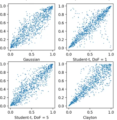
[image:28.612.207.400.226.424.2]

For intuition, we supply visualizations of copulas on the [0,1] square. We visu-alise the bivariate Gaussian copula, Student-t copula, and the Clayton copula in Figure 3.1. In this figure the marginal distributions are similar, so only the effect of the copula is visualised. Appendix A.3 shows the simulation algorithms for the different copulas depicted.

Figure 3.1: Comparison of several bivariate copulas.

The copulas depicted in Figure 3.1 share their rank correlation parameter.5 By this we are able to visualise the effect of the copula on the dependence structure. We see that the different copulas result in different dependence, this is explicitly visible in the tails.

5 _{Figure 3.1 shows a random sampling from the bivariate Gaussian copula with parameter} ρ= 0.9, from the bivariate Student-t copula with parameters ν =1 and ν = 5, ρ= 0.9

and from the bivariate Clayton copula with parameterθ=4.9654. The parameter for the

Clayton copula could be found via backwards by the analytic expression to calculate the Kendall tau.

For the Gaussian and Student-t copula, the formula for the Kendall tau is:

τ=2 πarcsinρ

For the Clayton copula, the formula for the Kendall tau is:

τ= θ θ+2

rewriting givesθ= 2τ

(29)

3.4 Chapter Conclusion

In this chapter we investigatedResearch Questions 2: “How can we model (correlated) defaults?”.

(30)

4

The 2008 global financial

crisis link with copulas

Now a decade ago, the financial system was rocked to its foundations. The great financial crisis observed in the period 2007-2009 was called the largest shock to the global economy since the Great Depression of the 1930s. In this chapter we mainly investigate the role of copulas within the financial crisis. The description of the 2008 global financial crisis and the role of copulas in this enables us to answerResearch Question 3.

(31)

[image:31.612.203.406.124.263.2]

Figure 4.1: CDO issuance over the period 1995-2017, data from: SIFMA (2018).

Route towards the crisis

After the global financial crisis the questions how things could turn out so bad was asked many times. Salmon (2012) states: “Investors like risk, as long as they can price it”. During the ’90s global financial markets expanded and trillions of dollars were waiting to be loaned to borrowers. The hard part was putting a number on the default correlation between all the loans made. Salmon describes that the one who solved this, “would earn the eternal gratitude of Wall Street and quite possibly the attention of the Nobel committee as well”. The need for a proper model was there, and after Li (2000) popularised the Gaussian copula model, the CDO market expanded quickly (see Figure 4.1).

MacKenzie (2011) describes one of the causes of the 2008 financial crisis as de-scribed hereafter.1 The CDO market expansion led to an increase of banking book size on the side of the financial institutions. Asset-backed security col-lateralised debt obligations (ABS CDOs) enabled the banks ability of buying risk exposures at a particular credit rating. Rating agencies (e.g. Standard & Poors, Moody’s, Fitch) rated the asset backed securities with high ratings since the idiosyncratic risk was diversified for the reason of being collateralised. Af-terwards, pooling of ABSs took place in the bank. At the banks the assumption again was that this ‘diversified’ the idiosyncratic ABS risk away. This second ‘diversification’ practice led to a low risk assumption, where in fact no extra risk was diversified. MacKenzie (2011) describes this as a“free lunch, eaten twice”.

1 _{The explanation of the causes on the global financial crisis by MacKenzie (2011) is only}

(32)

4.1. Copula adoption

4.1 Copula adoption

As we introduced in Chapter 3.2.2, Vaˇs´ıˇcek (1987) developed a widely-known model. The Vaˇs´ıˇcek model is able to model the loss distribution for large homo-geneous portfolios, given a single systematic risk factor. This model, known as the one-factor Gaussian copula (OFGC) model, became an industry standard for credit risk modelling from around 2000. The model was very convenient since when one underlying factor represents the state of the economy, the defaults by different companies could be treated as independent events (MacKenzie and Spears, 2014b).

The work of Vaˇs´ıˇcek on the Large Homogeneous Pool model was circulating through the banking industry, however it was never officially published (before the Journal of Risk published it in 2002). David Li: “I was aware of Vaˇs´ıˇcek’s work, I found that was one of the most beautiful math I had ever seen in prac-tice.” (MacKenzie and Spears, 2014b). The main problem of the Vaˇs´ıˇcek model according to Li was that it was a one period model. Li (2000) proposed a model which specifies the joint survival time distribution between marginal distribu-tions. Li (2000) enabled the application of copula functions to CDO tranche pricing, something which was not done before. With the copula function, Li was able to create a link between the marginal default distributions developing a joint default distribution for the CDO portfolios. By this, Li popularised the use of the Gaussian copula calibrated on market prices. In the years which fol-lowed, the work of Li would be applied in finance all around the world (Salmon, 2012).

We concisely list some of the essential reasons for applying copula functions to the world of finance:

• Copulas are popular because of their simplicity. When the marginals are known, they can be plugged into the copula function. This is a very convenient modelling practice.

• Many dependence structures could be modelled, since a wide range of dif-ferent copulas exists. A crucial point is however that one should accurately capture the dependence features of the data (Zimmer, 2012).

• The Gaussian copula was widely applied, which made it a good predictor of price movements (MacKenzie and Spears, 2014a).

• The Gaussian copula model became a widely applied model, this resulted in that also non-modellers (f.e. accountants) started favouring the model (MacKenzie and Spears, 2014a).

(33)

4.2. 2008 financial crisis

interviewed prior to the crisis). MacKenzie and Spears (2014b) reports in the pre-crisis interviews that quants were aware of the shortfalls of the Gaussian copula. The interviewees even described the method as unsatisfactory, and even not worth the term ‘model’ but an interpolation. The Gaussian copula model the situation was that there is a price derived from consensus: “Since everyone kind of uses the same model, .., everyone kind of agrees on the same price.” (MacKenzie and Spears, 2014b)

4.2 2008 financial crisis

In 2007, the financial world started to show cracks. When sub-prime lenders US started to default, it did not take long before housing bubble burst in 2008. In September 2008, Lehman Brothers collapsed. This event is seen as the defining event of the financial crisis, however it only was the start. The financial system was interwoven to a high degree, leading to a doom scenario for many financial institutions (FCIC, 2011). The recent developments and product innovations in the market of credit derivatives gave large exposures to portfolios of financial companies. Defaults rates rose to levels which were thought impossible with the Gaussian copula, which resulted in the fact that institutions faced risks which were much bigger than previously thought. For more conclusions on the causes of the financial crisis we refer to the document by the Financial Crisis Inquiry Commission in the US (FCIC, 2011).

In March 2009, Salmon wrote an article in technology magazine Wired, speci-fied on the application of the Gaussian copula model by David Li. The article headlined “Recipe for Disaster: The Formula That Killed Wall Street” (Wired, 2009). Salmon blames Li for applying the Gaussian copula formula to CDO pricing, concluding that Li’s instrument forced the global financial system to its knees. Salmon (2012) describes the advances of Li in the field of correlation modelling, what he did with a“simple and elegant mathematical formula”.

The main criticism from Salmon was on the specification of correlation structure. Li’s model based itself on CDS data to calculate correlations. CDS contracts had been in existence only for less than a decade, a decade in which house prices had soared. Salmon (2012) argues that this was a fatal flaw in the model of Li, since adverse price movement of house prices led to a different correlation number.

(34)

corre-4.3. Aftermath conclusions

lated events are asymptotically independent such that extreme events appear to be unrelated”. Zimmer (2012) argues that this drawback “might be innocuous in normal times, but not during extreme events such as the housing crisis”. The main conclusion after investigation on housing price data is that the Gaussian copula was unable to accommodate the tail dependence observed in the housing crisis.

4.3 Aftermath conclusions

Now, with the event of the great financial crisis a decade ago, it is time to re-flect. Salmon (2012) blames Li because his model assumed that correlation was a constant rather than a stochastic process. Another fatal flaw in the copula model of Li (2000) was the low tail dependence in the standard Gaussian copula application. Next to this, the fact that different CDO tranches had different implied correlations was counter-intuitive (and even impossible), since the CDO underlyings were the same.

MacKenzie and Spears (2014a) conclude that David Li cannot be blamed, and neither can the Gaussian copula in its essence be blamed. The Gaussian copula model is known for its shortfalls, the main thing that went wrong with this was the organizational process around it. Since all market participants (from investment banks to rating agencies and regulators) were using a similar model, it became the market standard for determining CDO prices. As long as the market stayed away from extreme situations, everything would go right. But when extreme events occurred, like the 2008 crisis, things would turn out very bad. On top of this, David Li came up with the explicit use of fully fledged cop-ula functions, but when the crisis hit in 2008 rating agencies had only moved partially into the direction of Li’s model (MacKenzie and Spears, 2014a).

We propose a proper overall conclusion where both Li, Salmon and Mackenzie & Spears would agree on: The work of Li on the Gaussian copula was a ‘recipe for disaster’ when users would not understand the essence and limitations of the model. Which got clear so far, is that the application of the static Gaussian copula model was at least partially blamed for the crisis. As a consequence, after the crisis richer correlation for credit risk approaches were introduced as dynamic copula models (Albanese et al., 2013).

(35)

4.4. The future with copulas: DRC

4.4 The future with copulas: DRC

Chapter 2 introduced the FRTB regulation and in specific the model require-ments for calculating the Default Risk Charge. In Chapter 3 we described how we could apply factor copula models to model default risk. However, after read-ing the critiques by e.g. Salmon (2012) on the (Gaussian) copula practices, the reader could pose himself the question why we would continue with the applica-tion of the Gaussian copula. We could write lengthy articles about this, but we want to keep the reasons clear and concise. We itemise several arguments for modelling the FRTB’s Default Risk Charge with a factor copula set up below:

• We know that the Gaussian copula approach lacks tail dependence. How-ever, DRC - IMA regulation prescribes that calibration of the parameters in the model should be covering a period of >10 years, including a pe-riod of stress. This implies that parameters are fitted to historical data including also bad economic times. On top of this, a market trading port-folio is almost never unidirectional. Because of this, the tails of the loss distribution are not per say matching the tails in the Gaussian copula.

• The critique of Salmon (2012) is on the Gaussian copula application on securitised financial products (CDOs). Within the FRTB regulation these products are directly subject to the standardised approach of the BCBS. Therefore, the modelling issues of capital charges for CDOs in an internal models approach are not applicable.

• The FRTB regulation prescribes backtesting methods for internal models. First, internal models are granted on desk level after proofs of correctness. Second, DRC-IMA models are subject to backtesting and P&L attribution procedures. This ensures that the regulator oversees whether modelling practices are done appropriately.

(36)

4.5 Chapter Conclusion

In this chapter we investigatedResearch Question 3: “Why did default mod-els not suffice in the 2008 financial crisis?”.

(37)

(38)

5

Modelling Default Risk

with LHP

In this chapter we describe our default risk model when we use the assumptions of the Large Homogeneous Pool (LHP) model by Vaˇs´ıˇcek. This chapter answers Research Question 4. The LHP by Vaˇs´ıˇcek is based on the one-factor Gaus-sian copula, we modify this into a Student-t and a Clayton copula model. We end this chapter by calibrating the different copulas on historical data, where-after we compare the differences between the copulas used for calibration.

5.1 LHP model

In Section 3.2.2 we described the model of Vaˇs´ıˇcek (1987). From here we con-tinue using the results of Vaˇs´ıˇcek (1987) to show the derivation of the Large Homogeneous Pool (LHP) approximation. The LHP approximation uses a one-factor Gaussian copula to represent the default correlation structure. The port-folio contains an infinite number of entities, which all have the same character-istics (e.g. PD, LGD, notional amount).

Below we show the derivation of the closed form result of Vaˇs´ıˇcek (1987). We use a slightly simplified notation compared to Section 3.2.2, changingP Di and ρi inP Dandρ. Equation 5.1 is the Vaˇs´ıˇcek LHP approximation (Bluhm et al.,

(39)

5.1. LHP model

G(x) =P(DR(F) ≤x) =P(Φ(

Φ−1(P D) −ρF √

1−ρ2

) ≤x)

=P( Φ−1

(P D) −ρF √

1−ρ2

≤Φ−1(x))

=P( −F≤ √

1−ρ2Φ−1(x) −Φ−1(P D)

ρ )

=P(F≥

Φ−1(P D) − √

1−ρ2Φ−1(x)

ρ )

=Φ( √

1−ρ2Φ−1(x) −Φ−1(P D)

ρ ) (5.1)

Here, G(x) represents the cumulative default distribution (CDF). After the CDF we want to derive the probability density function (PDF) for the default distribution. We do this by taking the derivative of the CDFG(x), this results in the PDFg(x)(Bluhm et al., 2010).

g(x) = ∂G(x)

∂x

= ¿ Á Á À1−ρ

2

ρ2 exp( − 1

2ρ2((1−2ρ 2

)(Φ−1(x))2−

2 √

1−ρ2Φ−1(x)Φ−1(P D) + (Φ−1(x))2) 2 ) = ¿ Á Á À1−ρ

2

ρ2 exp ⎧ ⎪ ⎪ ⎨ ⎪ ⎪ ⎩ 1 2(Φ

−1 (x))

2 −

1 2ρ2(

√

1−ρ2Φ−1(x) −Φ−1(P D)) 2⎫ ⎪ ⎪ ⎬ ⎪ ⎪ ⎭ (5.2)

LHP model with other dependence structures

(40)

5.1. LHP model

LHP with Student-t copula

A common approach to induce more tail observations than resulting from the normal distribution would be to work with a Student-t distribution. The same holds for copulas. The Gaussian copula has no tail dependence, where the Student-t copula does (whenν≠ ∞). Because of its capability of tail modelling, the Student-t copula is a widely applied copula in financial modelling (O’Kane, 2011).

Student-t copula approach by Schloegl and O’Kane (2005)

Schloegl and O’Kane (2005) extended the LHP approximation of Vaˇs´ıˇcek (1987). Where Vaˇs´ıˇcek assumed the asset returns are normally distributed, Schloegl and O’Kane (2005) assume that asset returns follow a multivariate Student-t distribution. The asset returnYi of asset i is:

Yi= √

ν Q(ρiF+

√

1−ρ2_iZi) (5.3)

Here F, and all Zi’s are independent, and N(0,1) distributed. Q is a χ2(ν) independent random variable withν degrees of freedom. The default condition

is: Yi<D. This could also be written as √

1−ρ2Zi≤D √

Q

ν−ρF. The portfolio

model could be interpreted as a mixing model. The mixing variable in this case

isη∶=D √

Q

ν −ρF. Now the conditional default probability can be written as

P r[Yi≤D∣η] =Φ( η √

1−ρ2

) (5.4)

Schloegl and O’Kane (2005) use the conditional default probability function to develop a cumulative distribution function for defaults. This method is how-ever computationally intensive and results in model complexity. Therefore we propose a Monte Carlo algorithm to model the cumulative default distribution for the Student-t copula approach for the LHP model.

Student-t copula approach using Monte Carlo

The Monte Carlo is set up by simulating the asset return Yi as formulated in

Equation 5.3. We write the default condition as: Yi < t−_v1(P Di). Using the formula for asset return Yi, we can write the conditional default probability

(41)

5.1. LHP model

DR(F, Q) =P r[Yi<t−_ν1(P Di)]

=P r[ √

ν Q(ρiF+

√

1−ρ2_iZi) <t−_ν1(P Di)]

=P r[Zi< √

Q νt

−1

ν (P Di) −ρiF

√ 1−ρ2_i

]

=Φ( √

Q νt−

1

ν (P Di) −ρiF

√ 1−ρ2_i

) (5.5)

By simulating the default rate (DR) 100.000 times, we obtain the distribution of default rates and we can present this in a CDF function. We come back to this in Section 5.2.2. Similar to what we showed for the Gaussian copula, we could also write the CDF and the PDF function for the Student-t copula. The CDF function is:

G(x) =Φ( √

1−ρ2_iΦ−1(x) − √

Q νt

−1

ν (P D)

ρi

) (5.6)

The PDF function is (Bluhm et al., 2010):

g(x) = ¿ Á Á À1−ρ

2

ρ2 exp ⎧ ⎪ ⎪ ⎨ ⎪ ⎪ ⎩ 1 2(Φ

−1 (x))

2 −

1 2ρ2(

√

1−ρ2Φ−1(x) − √

Q νt

−1

ν (P D))

2⎫ ⎪ ⎪ ⎬ ⎪ ⎪ ⎭

LHP with Clayton copula

The Clayton copula was introduced in Clayton (1978). The Clayton copula has dependence in the lower tail, which implies that extreme movements only cluster in one direction (Sch¨onbucher, 2002). So, the Clayton copula allows for occurrence of extreme downside events, this results in improved statistical per-formance compared to elliptical copulas (Low et al., 2013).

The CDF formula for Clayton copula one-factor model is (Sch¨onbucher, 2002):

F(q) =1−G( − lnq φ(p)

) (5.7)

Hereq represents the quantile at which we review the cumulative distribution,

φ()is the generator function for the Clayton copula, andpis the default prob-ability of any individual obligor.

From the CDF, the PDF formula for Clayton copula can be derived. This yields:

f(q) = 1

qφ(p) g( −

lnq φ(p)

(42)

5.2. Calibration of the LHP

Hereg(x)represents the Gamma distribution with parameterα. Hereα=1/θ, andθ is the parameter of the Clayton copula, (θ>0). The more the θ moves towards 0, the lower the dependence implied (Burtschell et al., 2009).

g(x) = αα

Γ(α)

xα−1exp(−αx) (5.9)

Since the Clayton copula is an Archimedean copula, we need a generator func-tion. The generator function for the Clayton copula is (Sch¨onbucher, 2002):

φ(p) = p−θ

−1

θ (5.10)

5.2 Calibration of the LHP

In this section we calibrate the LHP model. We start with the traditional LHP approximation, the Gaussian one-factor copula. Afterwards we do the same for the Student-t and the Clayton copula. We calibrate the models using the historical default rates per rating class. This is done by moment matching pro-cedures. We use historical data on default percentage per rating class by S&P for the period 1981 till 2016 (Standard & Poor’s Financial Services, 2017).

Please note the following things when reading the calibration of the LHP models hereafter. The visualization of the moment matching is based on default data on S&P rating category B.1 Rating categories are defined according to ‘S&P Domestic Long Term Issuer Credit Rating’. Appendix A.5 presents the complete data table on default rates per rating category for 1981-2016 (Table A.1) and the descriptive statistics (Table A.2).

5.2.1 Calibrating LHP - Gaussian

To calibrate the Gaussian one-factor copula, we apply a moment matching pro-cedure. The matching of moments is performed on the variance of the default rate. We first define the mathematical setup, before we show the calibration in practice.

Mathematical calibration method

Here we show our calibration method. The proof of this moment matching method is given by Gordy (2000), which is provided in Appendix A.4.

1 _{The procedure can also be applied to rating classes AA, A, BBB, BB and CCC/C. This}

(43)

Definition of variables:

N =Number of obligors

σ2=Variance of default

P D=Probability of default, for a rating class (avg. PD over a time frame)

Xi=N(0,1) asset return of obligor i

ρ=the correlation coefficient

σ(XiXj) =the covariance between obligorXiand Xj

Φ=Gaussian univariate distribution

Φρ=Bivariate Gaussian cumulative distribution value with parameterρ

We can write the variance of the mean default rate as the variance of a sum of correlated variables:

V ar(DR) = σ2 N +

N−1 N ρσ

2

= σ2 N +

N−1 N

σ(XiXj)

σ2 σ 2

= σ2 N +

N−1

N σ(XiXj) (5.11)

We know the following about the variance and the covariance:

σ2=P D(1−P D)

σ(XiXj) =Φρ(Φ−1(P D),Φ−1(P D)) −P D2

WhenN Ð→ ∞, Equation 5.11 changes since the first term drops. In this case we get:

V ar(DR) =σ(XiXj)

V ar(DR) =Φρ(Φ−1(P D),Φ−1(P D)) −P D2 (5.12)

For our calibration to the historical data we assume N Ð→ ∞, so we express Var(DR) as in Equation 5.12. Recall that we can calculate the first term in Equation 5.12 according to the Gaussian copula function.

Cρ(a, b) =Φρ(Φ−1(a),Φ−1(b))

= Φ−1₍_a₎

∫ −∞

Φ−1₍_b₎

∫ −∞

1

2π √

(1−ρ2)

exp{ − x2

+y2−2ρxy 2(1−ρ2)

}dx dy (5.13)

There are no analytic ways to compute the value of Equation 5.13, therefore we need another method to find the value. For this we program a function in our Python model which gets the arguments Φ−1

(44)

Practical calibration method

We continue with the practical calibration method. Previously we showed that we match the variance of the observed default rate (from historical data) with the variance rate resulting from Equation 5.12. To do the moment matching, we need inputs to our model. The inputs needed are unconditional PDs and the correlation factorρ.

We assume that unconditional PDs are published by S&P, this assumption is common when an IRB approach is not applicable (Rutkowski and Tarca, 2015).2 To find for whichρthe variance resulting from the data equals the variance re-sulting from Equation 5.12 we use Newton’s method, which is a root-finding algorithm.

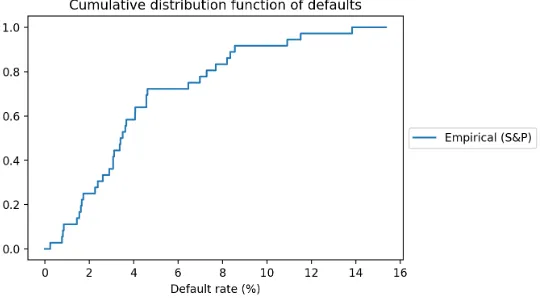
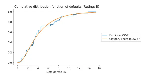
[image:44.612.171.441.351.500.2]

To get an insight in the defaults, we first plot the observed defaults. We plot a step function for observed defaults in Figure 5.1. We give an example how to read the graph: Figure 5.1 indicates that in 80% of the observed historical years, the default rate was equal to or lower than 8%.

Figure 5.1: Observed defaults for B rating.

Using the information from Figure 5.1 we calibrate a Gaussian copula to the observed data with our Python model. The one-factor Gaussian copula is the LHP model by Vaˇs´ıˇcek, for which we showed the derivation in Section 5.1.

P(DR(F) ≤x) =Φ( √

1−ρ2Φ−1(x) −Φ−1(P D)

ρ ) (5.14)

Here P D is the average probability of default on the data by S&P.DR is the default rate, which was also plotted on the horizontal axis in Figure 5.1. We

2 _“_{Where an institution has approved PD estimates as part of the internal ratings-based}

(45)

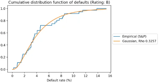
[image:45.612.171.442.162.304.2]

plot the formula for the default rates on the interval [0,16], the result obtained is presented in Figure 5.2.

Figure 5.2: Observed defaults for B rating and fitted copula function.

From Figure 5.2 we see that the Gaussian copula fits the empirical cumula-tive default distribution from the data well at first sight. We continue with calibrating the other copulas, in Section 5.4 we comment on the differences.

5.2.2 Calibrating LHP - Student-t

For the Gaussian and Clayton calibrations, we have analytic formulas for cali-bration. However as we described in Section 5.1 directly fitting to an analytic equation is not possible for the Student-t copula. The reason for this is that the analytic equations do not exist. Therefore we propose a simulation algorithm. From Section 5.1 we know that we can calculate the conditional default rate with Equation 5.15.

DR(F, Q) =Φ( √

Q νt−

1

ν (P Di) −ρiF

√ 1−ρ2_i

) (5.15)

By simulating the default rate many times, we can build a cumulative density function for the distribution of defaults. In every simulation run,F gets a ran-dom (normal) realisation and Qgets a random (chi-square) realisation. After 100.000 simulations, we construct the cumulative distribution function from the gathered data.

(46)

[image:46.612.163.441.117.263.2]

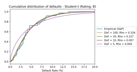
Figure 5.3: Calibration of Student-t copula to observed default rates.

As one can see from Figure 5.3 the calibration for a high degrees of freedom is almost analogous to the Gaussian/Clayton copula calibrations we saw before. For a low degrees of freedom the fit of the CDF is found by a very low ρ pa-rameter, providing a bad fit to historical data. When we compare the sum of squares from low ν with high ν, the sum decreases when we choose a higher degrees of freedomν.

To explain the effect of the Student-t copula compared to the Gaussian copula, we show the effect of having the sameρparameter various degrees of freedom. This implies a less good fit to the historical default rates, but ensures fatter tails. The effect is shown in Figure 5.4, the application is relevant for the DRC model in Chapter 6.

[image:46.612.172.441.450.589.2]

(47)

5.2.3 Calibrating LHP - Clayton

The calibration method for the Clayton copula in the LHP model is roughly the same as for the Gaussian model. The procedure here also involves moment matching, described in Section 5.2.1. Like for the one-factor Gaussian copula approach to the LHP model, we use a Newton method for the calibration pro-cess. Here we calibrate the Clayton copula parameterθ. The Clayton copula was described in Section 3.3.2. Equation 5.12 changes to Equation 5.16 for the Clayton copula.

V ar(DR) =φ−1(2φ(P D)) −P D2 (5.16)

Here φ(P D) is the generator for parameter P D. The generator function is φ(p) =p−θ−1 , as defined in Sch¨onbucher (2002). The inverse generator function is in this caseφ−1

(s) = (1+s)−1/θ. Using these results, we can calculateV ar(DR) from Equation 5.16 as:

V ar(DR) =φ−1(2φ(P D)) −P D2

=φ−1(2(P D−θ−1) −P D2

= (2P D−θ−1)−1/θ−P D2 (5.17)

We use Equation 5.17 in our root finding algorithm. As for the one-factor Gaus-sian copula, we match the observed variance from the data, with the variance according to Equation 5.17 for a certain value ofθ. From this method we find the optimised fitting parameter value.

To map the cumulative distribution of defaults, we use the formula below:

F(q) =1−G( − lnq φ(p)

) (5.18)

(48)

[image:48.612.156.444.117.266.2]

5.3. Empirical Evaluation

Figure 5.5: Observed defaults for B rating and fitted Clayton copula function.

In Figure 5.5 observe that the results look very similar to the Gaussian LHP approach. We come back to this in Section 5.4.

5.3 Empirical Evaluation

In this section we provide an empirical evaluation of the calibrations previously shown. We first provide confidence intervals for the data, afterwards we calibrate the copulas on the tails.

Building confidence intervals

We build confidence intervals around the data, since the data set contains only yearly observation points over 36 years. We build a confidence interval around the mean PD, and around variance of the PD. In Appendix A.6 we provide the methods for developing the confidence intervals in detail. Confidence intervals are shown for the Gaussian copula. Doing this for the Student-t or Clayton copula yields similar results, so we limit ourselves to one copula.

We build the confidence interval using formulas from statistics, next to this we compute confidence intervals with bootstrapping. The confidence interval for the mean PD is [4.25%,4.62%]. The confidence interval for the variance of the PD is [0.00052, 0.0016].

(49)

[image:49.612.160.446.119.254.2]

5.3. Empirical Evaluation

Figure 5.6: Fitted Gaussian copulas for 95% interval for the PD and PD variance.

From Figure 5.6 we can observe that the outer ranges of the copula calibra-tions lie around the observed historical data. This is a valuable result, since it visualises the uncertainty there implicitly is in the calibration.

Tail calibration

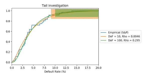
So far, we are calibrating the LHP models with the different copulas over the complete default distribution. However, in Chapter 4 we read that in 2008 the models were unable to model tail correlation correctly. For this reason, we perform a calibration on the tail in specific. From the historical default observa-tions, we should determine where the tail starts. We calibrate the model again with the tail start value at 9% default rate and at 10% default rate.

(50)

[image:50.612.159.444.117.262.2]

5.4. Comparison and inference

Figure 5.7: Calibration of the copulas on the tails

We see that the Student-t(ν=10, ρ=0.0046) copula fits the tail best when we determine the tail to starts at DR = 9%. However, when we determine the tail to start at DR= 10%, the Student-t(ν =100, ρ= 0.295) copula fits best. So, from Figure 5.7 we conclude that the determination of the start of the tail influences the copula which fits best. This result indicates that one should be aware of the copula function applied when calibration should be done on the tails of the default distribution. For example this is relevant when we work with unidirectional portfolios/strategies from (e.g.) hedge funds.

Lastly, it should be noted that a trading book portfolio is often multidirectional. This is an important difference between credit exposures in a banking book with similar exposures in the trading book. Since the trading books are not unidirectional, the 99.9% tail from the Gaussian copula does not necessarily correspond to the 99.9% tail of the loss distribution. We elaborate on this in the sensitivity analyses in Section 6.4.

5.4 Comparison and inference

In this section we compare the three different calibrations of the LHP models from Section 5.2. Afterwards we explain on this how we can infer the LHP model to a FRTB compliant model.

5.4.1 Visualizing the similarities

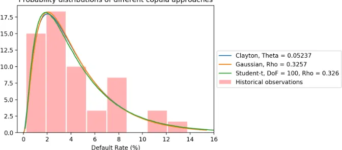
First, we visually observed that the Gaussian copula provides a good fit to the historical data plotted. After working out the Clayton and the Student-t copulas, we saw very similar calibration results on the CDF plots. By performing a least squares method for all copulas, we observe a lower sum of squares for the Gaussian copula than for the Clayton and Student-t copulas investigated.3

3 _{For a Student-t copula with very much degrees of freedom, the Gaussian case is reached.}

Modelling the FRTB’s Default Risk Charge with a factor copula setup

Master Thesis