Bayesian analysis of cointegrated vector autoregressive models

University of Warwick institutional repository:

http://go.warwick.ac.uk/wrap

A Thesis Submitted for the Degree of PhD at the University of Warwick

http://go.warwick.ac.uk/wrap/66201

This thesis is made available online and is protected by original copyright.

Please scroll down to view the document itself.

Autoregressive Models

By

Katsuhiro Sugita

A thesis submitted in partial fulfilment of the requirements for the

degree of Doctor of Philosophy in Economics

Department of Economics

University of Warwick

1 Introduction

1.1 Bayesian Analysis of Cointegration Models 1.2 Plan of the Thesis . . . .

12

12 16

2 Bayesian Cointegration Analysis 19

2.1 I n t r o d u c t i o n . . . 19 2.2 Bayesian Approach to Cointegrated Multivariate Time Series

Model - An Overview . . . 23 2.2.1

2.2.2

Posterior Information Criterion (PlC) . Kleibergen and Paap (2002) . . . . . 2.3 Bayesian Inference in Cointegration Analysis

2.3.1 Statistical Model . . . . 2.3.2 Prior and Posterior Distributions 2.3.3 The Griddy-Gibbs Sampler . 2.4 Bayes Factors for Cointegration Tests 2.5 Monte Carlo Simulation

2.6 Illustrative Examples . .

2.6.1 Cointegration Test for 'Great Ratios'

2.6.2 Cointegration Test for PPP and UIP 2.7 Conclusion...

50 56

3 Markov Switching Cointegration Model 58

3.1 I n t r o d u c t i o n . . . 58 3.2 Bayesian Estimation of the Markov Switching Cointegration

Model . . . .. 62 3.2.1 Markov Switching Cointegration Model with Two-Regime 62 3.2.2 Markov Switching Cointegration Model with m-Regime 64 3.2.3 Prior Distributions and Likelihood Functions.

3.2.4 Posterior Specifications . . . .

3.3 Testing for Markov Switching and Model Selection by Bayes Factors . . . .

3.4 Application: PPP between UK and US 3.5 Conclusion...

4 Cointegrated Models with Structural Breaks

66 68

73 83 89

91

4.1 I n t r o d u c t i o n . . . 91 4.2 A Time Series Model with Multiple Structural Breaks in

Co-integrated VAR Model 95

4.2.1 Statistical Model 95

4.2.2 Prior Distributions and Likelihood Functions. 97 4.2.3 Posterior Specifications and Estimation . . . . 99 4.3 Testing for Structural Break and Model Selection by Bayes

Factors . . . 106

4.5 Application: Japanese Term Structure of Interest Rates. 114 4.5.1 The Expectations Hypothesis . 114 4.5.2 Estimation Results

4.6 Conclusion .

5 Conclusion

5.1 Main Findings. 5.2 Future Research .

· 115 · 122

123

2.1 Posterior Density of

f3

for the 'Great Ratios' 48 2.2 Posterior Density of a for the 'Great Ratios' 48 2.3 Cointegration Relationship for the 'Great Ratios' 49 2.4 Posterior Densities of

f3

for the PPP & .UIP 53 2.5 Posterior Densities of a for the PPP & UIP 54 2.6 Cointegration Relationships for the PPP & UIP 55

3.1 Posterior expectation of the regime variable E[StIY] for UK/US PPP . . . , 88 3.2 Histogram of Posterior Densities for

f3*

(left) and a (alpha)

for UK/US PPP. . . .

4.1 An Example of a Simulated Series from DGP2

4.2 Posterior Probability Mass of the Break Dates - An Example from DGP2 . . . .

4.3 Japanese long-term and short-term interest rates. 4.4 Spread between Long- and Short-term Interest Rates

4.5 First Differences of Japanese Long- and Short-Term Interest 88

. 110

111 118 118

Rates . . . . . . . 119

4.6 Posterior Probability Mass of the Break Dates 4.7 Posterior Density of ,B2(left) and Cl! (right) ..

List of Tables

2.1 Evaluating Bayes Factors. . . .. 37

2.2 Monte Carlo Results:

t

=

50: Average Posterior Probabilities. 42 2.3 Monte Carlo Results:

t

=

100: Average Posterior Probabilities 43 2.4 Monte Carlo Results:

t

= 200: Average Posterior Probabilities 44 2.5 Cointegration Tests for the 'Great Ratios': Posterior

Proba-bilities . . . .

2.6 Bayesian Estimated (3* and a for the 'Great Ratios'

47 47 2.7 Cointegration Tests for PPP and UIP: Posterior Probabilities. 52 2.8 Posterior Results of (3* and a (,\

=

1.00) for PPP and UIP 52 2.9 Over-Identifying Restrictions on (3: values of Bayes Factors

for PPP and UIP . . .. 55

3.1 Average posterior probabilities: Testing for Cointegration,

Non-Cointegration and Markov Non-Cointegration . . 81

3.2 Average posterior probabilities for model selection 81 3.3 Monte Carlo Means for

13*

when the true model is M2 with

T=200 . . . . 82

3.4 Cointegration rank test (left) and Model Selection (right) 87

3.5 Posterior results for each parameter for M4 .

4.1 Monte Carlo Results: Average posterior probabilities 4.2 DGP2 - Estimation Results When m

=

2

4.3 DGP3 - Estimation Results When m

=

2

4.4 Parameter Estimates for Japanese Term Structure 4.5 Parameter Estimates for Japanese Term Structure

. . . 87

Acknowledgments

I am grateful to Mike Clements and Jeremy Smith for the continuous and patient guidance they have provided during the elaboration of this work.

This thesis has benefited from the comments and suggestions of partici-pants in the workshop "Recent Advances in Bayesian Econometrics" in Mar-seilles, the Econometric Society's Far Eastern Meeting in Kobe, the ESRC Econometrics Study Group annual conference at Bristol, the European Eco-nomic Association annual congress in Lausanne, SCE conference at Yale, and Royal Economic Society's annual conference at Warwick, the Econometric Workshop at University of Warwick, seminars at Birkbeck, Essex, Hitotsub-ashi Universities. I wish particularly to thank Luc Bauwens, Richard Paap and Christpher Sims for their comments on earlier versions of some parts of this work. I also wish to thank John Chao and Richard Paap to provide me with codes that were used in writing this thesis.

Declaration

Summary

This thesis concerns econometric time series modelling of cointegrated mul-tivariate systems using a Bayesian approach. The Bayesian approach has become increasingly attractive among researchers in the fields such as biol-ogy, though still only a relatively few econometricians use these techniques. Rather than theoretical aspects of Bayesian statistics or computational tech-niques, we illustrate how the Bayesian methods can be useful in analysing non-linear cointegration models.

In the last ten years, non-linear time series models, such as regime switch-ing models, have become popular among applied econometricians to analyse the business cycles, policy evaluation in specific macroeconomic issues and forecasting. Cointegration analysis has been influenced by the non-linearity so that cointegration models that allow regime switching or structural breaks have been analysed by many econometricians. Unfortunately, these non-linear cointegration models tend to be complicated both in terms of estima-tion and testing.

We consider in this thesis a Bayesian approach to (i) a linear cointegration model, (ii) a cointegration model with Markov regime switching, and (iii) a cointegration model with multiple structural breaks, and show how easily we can analyse these models without any substantial modification.

criterion, Kleibergen and Paap method, and one proposed method) for the cointegration rank. Provided we have enough large sample size, the Phillips' posterior information criterion gives consistent results, while the results by Kleibergen and Paap method depends on the prior hyperparameters that we specify.

In Chapter 3, we develop the cointegration model that allows cointegra-tion relacointegra-tionships to be switched on and off depending on the regime. Un-like the classical method that requires a two-step estimation, the Bayesian method provide a straightforward estimation and testing procedure.

Introduction

1.1

Bayesian Analysis of Cointegration Models

Since the prominent papers by Granger (1981) and Engle and Granger (1987), testing for and estimating cointegrating regressions has become an integral part of the tools of the applied economic researchers. Many methods have been developed using either residual-based single equation or multivariate system to determine these cointegrating relationships. Most of these methods are done using the frequentist approach, based on the asymptotic properties. Among these classical methods, the Johansen's trace test and maximum eigenvalue test have been most widely used.

In contrast, the Bayesian approach to cointegration models have been developed by only a few econometricians, see, for example, Koop (1991 and 1994), DeJong (1992), Dorfman (1995), Kleibergen and van Dijk (1994), Geweke (1996), Bauwens and Lubrano (1996), Chao and Phillips (1999), Kleibergen and Paap (2003), Strachan (2003), Villani (2003), Strachan and

Inder (2004).

As Maddala and Kim (1998) have noted, the Bayesian approach to coin-tegration has advantages over the classical methods. Firstly, it gives us finite sample results, while most of the classical methods rely on the asymptotic distributions. Secondly it avoids pre-testing problem which arises in the clas-sical methods. The pre-testing problem includes checking for unit roots for all variables in the model before undertaking the cointegration tests, and not knowing what effect these tests have on the significance levels used for the subsequent cointegration tests. Also, there is no definite answer to the question of what significance levels should be used for the unit root tests although it is conventional to use 5 percent and 1 percent significance levels. The ptesting problem can be avoided using Bayesian methods because re-spective posterior probabilities of unit roots and stationarity are taken into account.

Bayesian textbook that focuses on time series econometrics, and Koop (2003) is the first general Bayesian econometrics textbook which treats broad topic within econometrics such as panel data regression models, limited dependent variable models, time series models and nonparametric and semiparametric methods. The second reason is that Bayesian approach involves heavy com-putation both analytically and numerically. But, with recent development of algorithms for the Markov Chain Monte Carlo (MCMC) methods and avail-ability of faster computers has enabled us to undertake such complicated computation. The fourth reason is the lack of available computer packages for Bayesian techniques, meaning that one has to write ones own computer code if one wants to use Bayesian method. The final reason is that Bayesian method suffers from the controversy regarding to the choice of the prior den-sity. It seems that there is still no consensus about choosing appropriate priors for the unit root regressions. For this topic, Kass and Wasserman (1996) provide a critical survey of the different methods of generating prior distributions.

This thesis is not concerned with theoretical aspects of Bayesian cointe-gration analysis nor discussion of choice of the prior, but concerned with how Bayesian methods can be applied to analyse various types of cointegration models such as cointegration models with Markov regime switching or with multiple structural breaks in level, trend and error covariance.

parameters of the model are subject to Markov switching behavior, one has to estimate the parameters assuming the model is linear before unobserved regime variables are estimated, although the parameters are dependent on the regime variables. In the Bayesian analysis, both the parameters of the model and unknown regime variables are treated as random variables, and thus inference on the regime variables is based on a joint distribution. By using Gibbs sampling, both the parameters of the model and the unobserved regime variables are generated from appropriate conditional distributions.

10-cations of the break dates as the results of the Gibbs outputs of the posterior densities.

In this thesis we show how the Bayesian approach provides flexible and simple solutions for dealing with more complicated cointegration models with Markov regime switching in the level and the adjustment term and multiple structural breaks in the level, trend and error covariance.

1.2 Plan of the Thesis

In this section we provide a general outline of the thesis. The thesis con-sists of three chapters. Chapter 2 deals with linear cointegration models and evaluates three Bayesian testing methods for the cointegration rank using the Monte Carlo simulations. Chapter 3 is concerned with nonlinear coin-tegration models and applies the Bayesian method to evaluate a Markov switching cointegration model where the cointegrating relationships are sub-ject to regime switching behavior using a discrete first order Markov process. Chapter 4 applies the Bayesian approach to analyse a cointegration model with multiple structural breaks in level, trend and error covariance.

selecting the cointegration rank, assuming the true lag length is known. We present two illustrative examples - Great ratios and PPP - to see how these three methods give different results.

Chapter 3 introduces a Bayesian approach to a Markov switching cointe-gration model that allows the cointecointe-gration relationships to be switched on and off depending on the regime. We also consider a less restrictive Markov switching cointegration model in which deviations from the long-run equilib-rium are characterised by different rates of the adjustment depending upon the regimes. Unlike a classical method for nonlinear cointegration model that uses the cointegrating vector based on a linear cointegration model, the proposed Bayesian method allows for estimation of the cointegrating vector within a nonlinear framework conditional on the regime variables within the Gibbs sampling iteration. The Bayes factors are applied to test for Markov switching and model specifications. The PPP relationship between UK-US is investigated using the proposed model for illustration.

The model is applied to Japanese term structure data, and find that there is evidence of three structural breaks.

Chapter 5 summarises the main findings of this thesis and indicates

Bayesian Cointegration Analysis

2.1

Introduction

In the past decade, the econometric literature on cointegration has grown markedly since Granger (1981) introduced the concept of cointegration and Engle and Granger (1987) presented the Error Correction Model represen-tation and proposed a residual based test. Since then, many methods have been developed. For example, the FM-OLS procedure by Phillips and Hansen (1990), the dynamic OLS method by Saikkonen (1991), the nonlinear least squares by Phillips and Loretan (1991), the dynamic generalized least squares by Stock and Watson (1993). Among numerous procedures for estimation and testing for cointegration, lohansen's (1991) trace test and maximum eigenvalue test, based on canonical correlation in the system, have been most widely employed, and thus have been implemented in many econometrics packages such as EViews, Pc Give, Microjit, and others.

Several researchers have proposed Bayesian inference in cointegrated VAR

systems. Koop (1991) developed a Bayesian cointegration test using Monte Carlo integration techniques. He investigated the bivariate system of stock prices and dividends, tested for cointegration using posterior odds for hy-potheses, and found that there is evidence to support that unit roots are not present in stock price and dividend and thus there is no cointegration relationship between the two series even if unit roots are assumed. DeJong (1992) developed a method for evaluating the co-integration inference over trend stationary alternatives, and examined cointegration relationship be-tween consumption and income for the permanent income hypothesis. Dorf-man (1995) used a posterior odds ratio test for cointegration on the number of nonstationary roots in the system, and tested for cointegration among the exchange rates. Koop (1994) proposed a method based on the number of nonstationary roots in a VAR system.

of the singular values of IT. However, this informal visual inspection gives ambiguous results.1 Bauwens, et al (1999) suggest using the trace test of Jo-hansen, since "on the Bayesian side, the topic of selecting the cointegrating rank has not yet given very useful and convincing results"(p.283).

For more a formal Bayesian test for the cointegration rank, Kleibergen and Paap (2002) (KP, hereafter) proposed a method which uses a singular value decomposition of the unrestricted long-run multiplier matrix, IT, for identification of the cointegrating vectors and for Bayesian posterior odds analysis of the rank of IT. Chao and Phillips (1999) used the posterior infor-mation criterion (PlC, hereafter), proposed by Phillips and Ploberger (1994, 1996) and Phillips (1994a, 1994b, 1995, 1996), to select an appropriate model in terms of the rank and number of lags in the cointegrated VAR model.

Recent research by Strachan (2003) and Strachan and Inder (2004) criti-cised conventional prior with linear restrictions for the cointegrating vectors, and proposed a valid prior based on the cointegrating space. Strachan and van Dijk (2003b) applied this 'valid priors' to the VAR model. The choice of priors is also discussed by Strachan and van Dijk (2003a). Villani (2003) pointed out that the cointegration space is not an inner product space due to the well known non-identification of the cointegration vectors, and then proposed a Bayes estimator of the cointegration space that takes the curved geometry of the parameter space into account.

In this chapter we are interested in the performances of the two methods of KP and the PlC in the Monte Carlo simulations. We also introduce a

simple method for determining the cointegration rank by Bayes factors. The method is very straightforward, that involves computing the Bayes factors for each possible rank, and then selecting rank which has the highest Bayes factor. The procedure for obtaining the posteriors has some similarities with Bauwens and Lubrano (1996) method with conventional priors with linear restrictions on the cointegrating vectors. Although Strachan (2003) criticised this prior for the cointegrating vectors as invalid, we follow the conventional prior in this thesis. We consider Strachan's method for the future research. While the method is not invariant with respect to the ordering of the vari-ables in the VAR, it is able to determine the correct cointegrating rank. We conduct Monte Carlo simulations to compare this simple method with the KP method or PlC.

purchasing power parity (PPP) are presented. Section 2.7 concludes.

2.2

Bayesian Approach to Cointegrated

Multi-variate Time Series Model - An Overview

We review briefly in this section cointegration tests by Phillips PlC and the KP method.

2.2.1

Posterior Information Criterion (PlC)

For model selection, the Akaike information criterion (AIC) or Schwarz's Bayesian information criterion (SBIC), which impose a penalty based on the dimension of the selected model, are most widely used (for example, to select the lag length in the model). Phillips and Ploberger (1994, 1996) and Phillips (1994a, 1994b, 1995) proposed an alternative criterion for model selection, called the posterior information criterion (PlC). The PlC explicitly depends on the data matrix, unlike both the Schwarz BIC and AIC which depends on the number of regressors and the residual variances. To select an appropriate model of the regression among different models M = 1, ... , k,

YM

=

XM f3M +E, we compute the PlC for all models M

=

1, ... , k, and then select a model which has the lowest value of the PlC. The PlC is computed as follows:

(2.1)

o:1r

is the maximum likelihood (ML) estimate of the error variance, and

/3M

is the ML estimate of the coefficient vector.

Chao and Phillips (1999) extended the PlC to cointegrated models to select both the lag length

p

and the number of rank f jointly. They stressed this joint test since the performance of cointegration test such as Johansen (1992) can be adversely affected by lag misspecification as shown by Toda and Phillips (1994).

Consider the n-dimensional vector autoregressive process of order p

+

1 Yt

=

<I>(L)Yt-l

+

Et (2.2)

where <I>(L)

=

L;r~;<I>iLi-l. Eq. (2.2) can be written in vector error correction model (VECM) representation as

(2.3)

where I1*

=

<1>(1) - In

=

a{3' with a and {3 are n x r matrices, and <1>*(L) =

"p+l;r.*Li -1 _{·th;r.* -} "p+l <1> . - 1

L...i=l '±'i Wl '±'i - -L...rn=i+l rn, Z - , . . . ,po

Let Y

=

[Y1, ... , YT ]', Y-1

=

[Yo, ... , Yt-l]', .6.Y

=

[.6.Y1 , ... , .6.YT ]' and W(P)

=

[W1(P), ... , WT(P)]' with Wt(P)

=

[.6.Yf-l,"·' .6.Yf_p ]', W(P)

=

[W(p) W(P*)] where W(P) contains the first np columns and W(p*)

~Y'~Y ~Y'Y-l ~Y'W(p) ~Y'W(p*)

S Y~l~Y Y~lY-l Y~lW(P) Y~l W(p*)

W(p)'~Y W(P)'Y-l W(P)'W(p) W(p)'W(p*)

W(p*)' ~Y W(P*)'Y-l W(p*)'W(p) W(p*)'W(p*)

St,.t,. St,.y St,.p St,.po

Syt,. Syy Syp Sypo

Spt,. Spy Spp Spp'

Spot,. _{Sp.y SP'p Spop'}

St,.t,. St,.y St,.p

Syt,. Syy Syp

Spt,. S-py Spp

Define Sij.k

=

Sij - SikSkk1 Skj for i, j

=

~,y and k

=

p,

p,

and Sij.k.l

=

Sij.k - Sil.kSil.kSlj.k for i.j

=

~,p* and k, l

=

y, p,

P-To estimate the cointegrating rank, r, and the lag length, p, jointly, we select

(ft,

f) as follows:

(ft,

f) = argminPIC(p, r)

where

(2.4)

where

iL(p,

r)

[&(p,r),&(p,r)~(p,r)']

with &(p,r) and

~(p,r)

are the maximum likelihood estimators of the parameters a and

73

when the coin-tegrating rank is assumed to be r and the number of lags is assumed to be p,

ft

(p)

=

S

D.y.pS;;y~p

and

IT*

(p*)

=

S D.p' .y.pS;'p' .y.p'

~

is the

maxi-mum likelihood estimator of I;, and the (2nr - r2) x n2 matrix H(p, r) =

[(&(p, r)' ® F(r)')', (In ®

(IT~(P'

r),))IJ'.

Chao and Phillips (1999) criticized Johansen's sequential procedure of testing the cointegrated rank from the subhypothesis r

=

0 onwards as the procedure does not yield a consistent estimator of the cointegrating rank. Another advantage to the PlC is that the penalty function of the PlC takes into account not only the number of parameters (like AIC and SBC) but also the nonstationarity of the regressors associated with some of the parameters. However, the procedure is not completely Bayesian because some pa-rameters rely on the maximum likelihood estimators. Also, unlike Bayesian posterior odds analysis, the PlC does not provide uncertainty among models that we consider (see Phillips, 1995, the comments, and Phillips' reply).

2.2.2 Kleibergen and Paap (2002)

by using a singular value decomposition to construct a parameter that reflects the presence of rank reduction.

Suppose we are considering the VECM of the form:

p-l

b.Xt

=

J-L

+

il' Xt -1

+

L

Wib.Xt -i

+

et, (2.5)

i=l

KP decomposed the long-run multiplier, il, as follows:

where a-L and f3-L are specified such that a-La'

==

0 with a-La~

==

In-r and f3~f3== 0 with f3~f3 -L

==

In - r . When).

=

0, the long-run multiplier il shows

rank reduction and the model has some cointegrating vectors. By

apply-~

a::

e

:in:l:

:ru:eor:::::~~:ti:at:c~'

w::

h:V~

IT[

:1~ 8~~

lW::

U21 U22

V

=

[vn

V12], and 8 is an n x n diagonal matrix containing the non-V21 V22

[ 81 0

l'

negative singular values with decreasing order such that 8 =

o

82

Un, 81 , and ViI are r x r matrices, U22 , 82 and V22 are (n - r) x (n - r)

matrices, _{U21 and 1121 are} (n - r) x r matrices, and U12 and V12 r x (n -r) matrices. Then, we have a

=

Un 8 n [Vn, V21 ]',

f3

=

-U21 Uli\ ).

=

(Metropo-lis et al (1953) and Hastings (1970)) can be implemented to generate posterior output instead of using the standard Gibbs sampling because the full condi-tional posterior distributions are of unknown type. Testing the cointegration rank is done by the posterior odds, and the Bayes factors are computed using the Savage-Dickey density ratio (Dickey, 1971) by imposing>..

=

0 as the null hypothesis.

KP chose the conjugate priors, the inverted Wishart for the covariance matrix L: and the matric variate normal for IT conditional on L:, and the g-prior of Zellner (1986) for the prior covariance for IT. The joint prior on the parameters in the cointegration model is obtained by putting the ma-trix reflecting the presence of rank reduction (>.. = 0) such that p(L:, a, (3) ex: p(L:, IT) III=.Ba IJ(IT, (a, >.., (3)I>.=owhere IJ(·)I>.=o denotes the Jacobian trans-formation evaluated in >..

=

O. In case of diffuse (non-informative) prior speci-fication, KP asserted that by taking an appropriate prior height (21T")-1/2(n-r)2,

the Bayes factor is equivalent to the PlC.

2.3 Bayesian Inference in Cointegration

Anal-.

YSlS

2.3.1 Statistical Model

In this section we present a simple Bayesian analysis of cointegration, ex-tending Bauwens and Lubrano (1996). Let

X

t denote an

1(1)

vector of

p-l

.6.Xt = J-L

+

It

+

oJ3'Xt -1

+

L

Wi.6.Xt -i

+

Ct (2.7)

i=l

where t = p, P

+

I, ... , T, p is the number of lags in VAR, and the errors, ct, are assumed N (0,

2::)

and independent over time. J-L, I, c, W, L:;, a, and (3 are parameters of dimensions n x I, n x I, n x n, n x n, n x r, and n x r, respectively.

Equation (2.7) can be rewritten in matrix format as:

Y

=

Xf

+

Z (3' a'

+

E

=

W B

+

E (2.8)

where

J-L'

.6. X , _{X;_l c'}

p p

!'

.6.X;+l X'

,

y=

,

Z=

p

,

E-

-

cp+l , f=

_W'

1

.6.X~ X~_l

W~_l

1 p .6.X;_l .6.X~

1 p+1 .6.X' .6.X~

X= p

1 T .6.X~_l .6.X~_P+l

B=

[ :' 1

Let m be the number of rows of Y, so that m

=

T - p

+

1, then X is mX(2+n(p-1)) , f ((2+n(p-1))xn) , W (mxk), where k

=

2+n(p-1)+r,

format of (2.7). This representation is a starting point. We then describe the prior and likelihood specifications in order to derive posteriors.

2.3.2 Prior and Posterior Distributions

In this subsection, we consider a Bayesian estimation of the vector error correction models presented in (2.7). The conjugate prior density for B conditional on covariance L: follows a matrix-variate normal distribution with covariance matrix L: ® A -1 of the form

p(B

I

L:) ex 1L:I-k

/2IAln/2 exp

[-~tr

{L:-1 (B - P)' A (B - P)}] (2.9)

where A is (k x k) PDS and P (k x n), k

=

n(p - 1)

+

r

+

1 (the number of columns in W ).

For the prior density ofthe covariance L: in (2.8), we can assign an inverted Wishart

(2.10)

where h represents the degrees of freedom, San n x n PDS. Instead of above priors, if we do not want to impose an informative prior for L:, we can opt diffuse prior for L: as p(L:) ex 1L:1-(n+l)/2.

1f

(/3)

ex: IQI-n/2IHlr/2 exp

[-~tr

{Q-l

(/3

-73)'

H

(/3

-~)}]

(2.11)

where ~ is a prior mean of

/3,

Q is r x r PDS, His n x n PDS. Note that r2 restrictions for identification are imposed on

/3,

for example,

/3'

=

(I

_r /3~ ),2 where

/3*

is (n - r) x r unrestricted matrix. If we assign r2 restrictions on

/3

as In then only a part of

/3, /3*,

follows a matrix-variate normal.

If we assume that Band L: are independent of

/3,

then the joint prior of the parameters in (2.8) is p(B,

/3,

L:) ex: p(BIL:)p(/3)p(L:) and thus can be derived as

p(B,

L:,

(3) ex: 1f

(/3)

IAln/21L:1

k t h t ' t l exp

[-~tr

{L:-

1 [8

+

(B - P)' A(B - P)J}]

(2.12) To derive the conditional posterior distributions, we need to derive the likelihood functions. The likelihood function for B, L:, and

/3

is given by:

L (Y

I

B,

L:,

(3) ex:

1L:I-

t/

2

exp [-~tr

{L:-

1 (Y - W B)' (Y - W B)}]

(2.13)

ex:

1L:I-

t/

2

exp {

-~tr

[L:-

1

{S

+

(B - E)'W'W(B - E) }]}

where

13

=

(W'W)-lW'Y, and

S

=

(Y - WE)'(Y - WE).

Next we derive the posteriors from the priors and the likelihood function specified above. The joint posterior distribution for the conjugate priors for

B, I; and f3 is proportional to the joint prior (2.12) times the likelihood function (2.13), thus we have

p (B, I;, f3 I Y) ex. p (B, I;, f3) L (Y I B, I;, f3)

ex. 1r (f3) IAI%'II;I-(t+h+k+n+l)/2

X exp

[-~tr

{I;-l [S

+

(B - P)'A(B - P)

+ S +

(B - 13)'W'W(B - 13]}]

ex. 1r (f3)

II;I-~

exp

[-~tr

{I;-l [S

+

S

+

(P - 13),[A-1

+

(W'W)-ltl(p -

B)

+(B - B*)'A*(B - B*)])]

= 1r (f3)

II;I-~

exp

[-~tr

{I;-l [S*

+

(B - B*)'

~(B

- B*)]}] (2.14)

where c

=

t+k+h+n+1, ~

=

A+W'W, B*

=

(A+W'W)-l(AP+W'W13),

and S* = S

+ S +

(P - B)'[A-1

+

_{(W'W)-l]-l(P -}

B).

From (2.14), the conditional posterior of I; is derived as an inverted Wish art distribution, and the conditional posterior of B as a matrix-variate normal density with covariance, I; ® A;l, that is,

p(B I I;, f3, Y) ex. IA*ln/21I;I-k/2 exp

[-~tr

{I;-l(B - B*)'A*(B - B*)}]

Thus, by multiplying (2.15) and (2.16), and integrating with respect to ~, we obtain the posterior density of B conditional on (3, which is a matrix-variate Student-t form,

(2.17)

The joint posterior of Band (3 can be derived by integrating (2.14) with respect to ~,

(2.18)

By integrating (2.18) with respect to B we obtain the posterior density of the cointegrating vector (3,

(2.19)

The properties of (2.19) are not known, so that we have to resort to numer-ical integration te~hniques, as Bauwens and Lubrano (1996) used importance sampling to compute poly-t posterior results of the parameters. Other fea-sible methods are the Metropolis-Hastings algorithm and the Griddy-Gibbs sampling. The Metropolis-Hastings3 _{algorithm requires the assignment of a}

good approximating function, the candidate-generating junction, to the pos-terior to draw random numbers, as importance sampling requires the

tance function. Since the Griddy-Gibbs sampling method does not require such an approximation, we employ the Griddy-Gibbs sampler for estimation of the cointegrating vector (Bauwens and Giot (1998) used this sampler for the estimation of two cointegrating vectors).

2.3.3 The

Griddy-Gibbs

Sampler

The Griddy-Gibbs sampler, proposed by Ritter and Tanner (1992), approx-imates the true cdf of each conditional distribution by a piecewise linear function and then samples from the approximations. This sampler can be implemented when the conditional posterior density is unknown to the re-searcher. The disadvantage of this sampling method is that the results are depending upon how we assign the range and the number of the grid for the parameter. The range should be chosen so that the generated numbers are not truncated. Another disadvantage is that this sampler demands more computing time than other algorithms. The advantage of using this sampler over the importance sampler or the Metropolis-Hastings algorithm is that researcher does not have to provide an approximation of the function. The procedure for implementing the Griddy-Gibbs sampler is as following:

1. Before we begin the chain, we must choose the range of the grid and the number of the grid. The range should be chosen so that the generated numbers are not truncated.

f3l,l

is the lower bound of the grid of

f3l,

and

f3l,U

is the upper bound of the grid of

f3l.

3. Compute the values G = (0, <I> 2 , <I>3,"" <I>u) where

r

f31_,j

<I>j

lA

f(f3llf3~,f3~,··.,f3:n,Y)df3l

f31,1

j

=

2, ... ,U

4. Compute the normalized pdfvalues G(

=

Gj /<I>u of ((f3llf3~, f3~,

... ,f3:n, Y).

5. Draw the random numbers from the uniform density with the lower bound as zeros and the upper bound as <I>u and invert cdf G by numer-ical interpolation to obtain a draw

f3t

from ((f3llf3~, f3~,

... , f3:n, Y).

6. Repeat steps 2-5 for

f32' ... ,f3m.

7. Set i

=

i

+

1 (increment i by 1) and go to step 2.

Note that integration at the step 3 can be done by the deterministic approx-imation such as the Simpson's rule or the Trapezoidal rule.

2.4 Bayes Factors for Cointegration Tests

model represents the truth and the test is based on a pairwise comparison with the alternative. For a detailed discussion of the advantages of Bayesian methods, see Koop and Potter (1999). Kass and Raftery (1995) provide an excellent survey of the Bayes factor.

Suppose, with data Y and the likelihood functions with the parameters 8, there are two hypotheses Ho and H1 • The Bayes factor BFol is defined as follows:

Pr(YIHo)

Pr(YIH1)

J

p(8I Ho)L(YI8, Ho)d8

J

p(8I Hl)L(YI8, Hdd8 (2.20)

With the prior odds, defined as Pr(Ho)/Pr(H1), we can compute the posterior odds, which are

. Pr(HoIY) Pr(YIHo) Pr(Ho)

PostenorOddso1

=

Pr(H1IY)

=

Pr(YIH_{1) . Pr(H1)} (2.21)

When several models are being considered, the posterior odds yield the pos-terior probabilities. Suppose q models with Ho, H1 , ... , Hq - 1 are being

con-sidered, and each of the hypotheses H1 , H2 , ••• ,Hq- 1 is compared with Ho. Then the posterior probability for model i under Hi is

Pr(HiIY)

=

P~steriorOddsio

2:j:o PosteriorOddsjo (2.22)

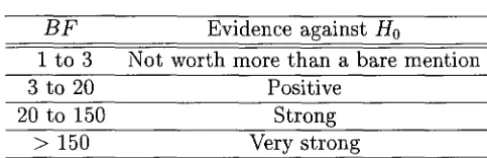
fore-Table 2.1: Evaluating Bayes Factors

This table was reproduced from Kass and Raftery (1995)

BF

Evidence against Ho

1 to 3 Not worth more than a bare mention

3 to 20 Positive

20 to 150 Strong

>

150 Very strong

casting. A rule of thumb for interpreting the magnitude of a Bayes factor provided by Kass and Raftery (1995) is reproduced in Table 2.1 for conve-nience.

There are several methods to compute the Bayes factors given in (2.20). For example, the Laplace approximation method (Tierney and Kadane, 1986), or using numerical integration techniques such as importance sampling (Geweke, 1989) or the Metropolis-Hastings algorithm. See Kass and Raftery (1995) for details. Chib (1995) proposes a simple approach to compute the marginal likelihood from the Gibbs output. Newton and Raftery (1994) suggested us-ing the posterior density p( ()

I

Y) as the importance function because samples from the posterior density arise directly from the Gibbs sampler, so that the marginal likelihood for model j (Mj) can be simplified to the harmonic mean of the likelihood as:

(2.23)

where ()(k) , k

=

1, ... , N, are sample draws from the Gibbs sampler. An

[image:39.564.157.401.179.258.2]

Yao (1988) and Liu et al (1997) suggested:

(2.24)

where

~

(0;

I

Y; Mj ) denotes the likelihood function under the model j; qj

denotes the total number of estimated parameters in the model j; M_j denotes the model indicator for model j. The likelihood function

~

(0;

I

Y; Mj ) is

evaluated at ()j, the posterior means of the parameters for model j. The Bayes factor for model k against model j can be approximated by

(2.25)

In this chapter we use two algorithms in (2.23) and (2.25) to detect the rank in cointegrated VAR model. Note that our method is not invariant with respect to ordering of the variables in the VAR, and thus the values of Bayes factors depend on the ordering, although, the values should reflect the correct rank.

2.5 Monte Carlo Simulation

To illustrate the performance of Bayesian tests for the rank of cointegration described in the previous section (2.3 - 2.4), we perform some Monte Carlo simulations. The data generating processes (DGPs) consist of a four-variable VAR with an intercept term having various number of cointegrating vectors (0, 1, 2, 3 and 4) as following:

2. (r

=

1) !::::. Yt

=

J.l

+

3. (r

=

2) !::::. Yt

=

J.l

+

-0.2

[ 1 0 0 -1 ] Yt-l

+

et

-0.2

-0.2

0.2

-0.2 -0.2

0.2 -0.2

0.2 0.2

-0.2 0.2

-0.2 -0.2 -0.2

0.2 -0.2 -0.2

o

0 1 0

-1

1

-1

Yt-l

+

et

4. (r

=

3) !::::. Yt

=

J.l

+

1 0 0

0 1 0

0 0 1

-11

-1 Yt-l

+

et

5. (r = 4) !::::. Yt = J.l

+

0.2 0.2 -0.2

0.2 0.2 0.2

-0.2 -0.2 -0.2 -0.2

0.2 -0.2 -0.2 -0.2

0.2 0.2 -0.2 -0.2

0.2 0.2 0.2 -0.2

-1

1 0 0 0

o

1 0 0

0 0 1 0

0 0 0 1

where J.l

= [

0.1 0.1 0.1 0.1

r

and et rv NID(O, h).

Yt-l

+

et

In these experiments, we also run the Monte Carlo simulations for the PlC and the KP method described in Section 2.2. The PlC does not depend on the prior distributions. Note that the PlC does not provide any posterior probability so that interpretation from the Monte Carlo simulations is not the same as from the other Bayesian methods.

The prior parameter specifications for the natural conjugate priors are as follows: P = 0 and A = h/1000 in (2.9),

7J

=

/3,

Q = In , H = h/1000 in

(2.11), S

=

14/1000 in (2.10) to ensure fairly large variance for representing

prior ignorance. For the KP method, we assign ()

=

1 and 0.01 in (}(X'X)/t,

which is the prior variance of IT and g-prior of Zellner (1986), to see how this prior specification affects the results because this method uses the Savage-Dickey density ratio to compute the Bayes factor and thus it is very sensitive in choosing the prior parameters, while the Bayes factors by the methods in (2.25) and (2.23) are insensitive in the hyperparameters. Note that a smaller value of () implies less prior information.

selected. The column labeled as PlC is not the average posterior probability because the PlC does not offer posterior odds (model uncertainty) so that each elements is the frequency that each rank is chosen.

Tables 2.2 - 2.4 show that the PlC tends to select lower rank than the true rank especially when the sample size is 50 and 100. For example, with t

=

50 and full rank, the PlC selects a correct rank with only 13.6 per cent. However, with t

=

200, the PlC shows the best performance in our simulations among all methods we consider. This PlC's sample size sensitivity would be caused by the fact that the criterion uses the maximum likelihood estimators.

For the KP method, it is clear that the method is quite sensitive in the choice of the prior hyperparameter

e.

The lower

e,

the method tends to choose lower rank. The method with diffuse priors shows much better performance in our simulations, although it performs as poorly as the PlC when the sample size is small.

BF1 also tends to select lower rank than the true rank when the sample size is small. This method also performs worse than BF2 when the sample size is small. However, BF2 shows slightly better performance than BF1.

Table 2.2: Monte Carlo Results:

t

= 50: Average Posterior Probabilities I True rank rank r I PlC Kpl KP2 Kp3 _{BFl BF2 I}

r=O 0 0.924 0.315 1 0.078 0.288 2 0.001 0.197 3 0.000 0.122 4 0.000 0.079

r=l 0 0.267 0.009 1 0.702 0.299 2 0.030 0.307 3 0.001 0.229 4 0.000 0.156

r=2 0 0.001 0.000 1 0.329 0.033 2 0.630 0.181 3 0.038 0.450 4 0.001 0.336

r=3 0 0.003 0.000 1 0.213 0.002 2 0.501 0.121 3 0.276 0.447 4 0.007 0.430

r=4 0 0.001 0.000 1 0.188 0.001 2 0.439 0.056 3 0.236 0.262 4 0.136 0.681 Note:

PlC: Posterior Information Criterion

Kpl: Kleibergen and Paap method with (} = 1.00

KP2: Kleibergen and Paap method with (} = 0.01

Kp3_{: Kleibergen and Paap method with diffuse prior}

BF1: uses the Schwarz BIC given in (2.25)

1.000 0.000 0.000 0.000 0.000 0.982 0.018 0.000 0.000 0.000 0.244 0.573 0.167 0.013 0.003 0.325 0.433 0.211 0.023 0.008 0.227 0.473 0.226 0.038 0.036

BF2: uses the harmonic mean of the likelihood given in (2.23) Johansen: the numbers are p-values by Johansen's trace test

[image:44.569.117.433.156.512.2]

Table 2.3: Monte Carlo Results: t = 100: Average Posterior Probabilities

I

True rank rank r

I

PlC Kpl KP2 Kp3 _{BFl BF2}

I

r=O 0 0.995 0.688 1 0.005 0.213 2 0.000 0.065 3 0.000 0.023 4 0.000 0.011

r=l 0 0.011 0.000 1 0.984 0.610 2 0.005 0.263 3 0.000 0.091 4 0.000 0.036

r=2 0 0.000 0.000 1 0.020 0.006 2 0.974 0.319 3 0.006 0.414 4 0.000 0.262

r=3 0 0.000 0.000 1 0.006 0.000 2 0.487 0.032 3 0.505 0.601 4 0.002 0.365

r=4 0 0.000 0.000 1 0.003 0.000 2 0.278 0.005 3 0.367 0.093 4 0.353 0.902 Note;

PlC; Posterior Information Criterion

Kpl; Kleibergen and Paap method with fJ = 1.00 KP2; Kleibergen and Paap method with fJ = 0.01 Kp3_{; Kleibergen and Paap method with diffuse prior}

BFl; uses the Schwarz BIC given in (2.25)

1.000 0.000 0.000 0.000 0.000 0.468 0.532 0.000 0.000 0.000 0.000 0.165 0.782 0.043 0.011 0.000 0.134 0.624 0.229 0.013 0.000 0.100 0.445 0.138 0.318

BF2; uses the harmonic mean of the likelihood given in (2.23) Johansen; the numbers are p-values by Johansen's trace test

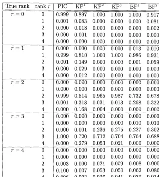
[image:45.569.119.431.157.509.2]

Table 2.4: Monte Carlo Results: t = 200: Average Posterior Probabilities

I

True rank rank r

I

PlC Kpl KP2 Kp3 _{BFl BF2}

_I

r=O 0 0.999 0.897 1 0.001 0.083 2 0.000 0.018 3 0.000 0.001 4 0.000 0.000

r=l 0 0.000 0.000 1 0.999 0.810 2 0.001 0.149 3 0.000 0.029 4 0.000 0.012

r=2 0 0.000 0.000 1 0.000 0.000 2 0.999 0.514 3 0.001 0.318 4 0.000 0.168

r=3 0 0.000 0.000 1 0.000 0.000 2 0.000 0.001 3 1.000 0.720 4 0.000 0.279

r=4 0 0.000 0.000 1 0.000 0.000 2 0.003 0.000 3 0.100 0.007 4 0.896 0.993 Note:

PlC: Posterior Information Criterion

KP1: Kleibergen and Paap method with () = 1.00 KP2: Kleibergen and Paap method with () = 0.01 Kp3_{: Kleibergen and Paap method with diffuse prior}

BF1: uses the Schwarz BIC given in (2.25)

1.000 0.000 0.000 0.000 0.000 0.000 1.000 0.000 0.000 0.000 0.000 0.000 0.965 0.031 0.004 0.000 0.000 0.236 0.712 0.053 0.000 0.000 0.021 0.053 0.926

BF2: uses the harmonic mean of the likelihood given in (2.23) Johansen: the numbers are p-values by Johansen's trace test

[image:46.569.114.433.157.512.2]

2.6 Illustrative Examples

In this section, we illustrate two examples of cointegration analysis using the method that is presented in previous sections. The main focus is to show the usefulness of our method with a relatively small number of observations and to compare it with other methods such as the PlC, the KP method and Johansen's test. The first example is a cointegration test for 'great ratios'. The second is for UK's PPP (purchasing power parity) and UIP (uncovered interest rate parity).

2.6.1

Cointegration Test for 'Great Ratios'

King et al (1991) (KPSW) examined cointegrating relationships between US output (Y), consumption (C), investment (1), and three other variables. In this sub-section, we investigate a three-variable model containing the real variables, C, I and Y. The data are quarterly and taken from the KPSW data set, which are: C (real per capita consumption, in logs), I (investment per capita, in logs), and Y (real private output per capita, in logs). We choose the shorter estimation period of 1968 (1) - 1988 (4), with a sample size of 83 to see how various tests choose the rank when the sample size is small. From economic theory, two cointegrating relations are expected to be found among these variables, given by C - Y and 1-Y, which are known as the 'great ratios'.

(2.25) and (2.23), and Johansen's trace test, with 2 lags4 _{in VAR for the}

three-dimensional vector of time series

yt

= [ C_t It

yt]

with an intercept term. The prior specifications are the same as those used in the simulations. Thus, these prior hyperparameters favour no cointegration but are relatively noninformative given the fairly large variance. We assign an equal prior probability to each rank. We also impose restrictions on the cointegrating vector as

f3

=

(IT f3*)

for both identification and normalisation. From Table 2.5, most of the Bayesian tests show that the posterior probabilities for rank 1 are the highest for the PlC, Kpl (with () = 1.00), Kp3 _{(with diffuse}

priors) and two BFs, while KP2 (with () = 0.001) selects rank O. There is almost no evidence of rank 2 or 3. The Bayesian tests find that there is a cointegration relationship between consumption and income, but not between investment and income, although KPSW found two cointegration relationships using full data set. On the classical side, Johansen's trace test cannot reject r = 0 at either 5 or 10 per cent significance level.

Table 2.6 shows the posterior results of

f3*

and n. If we assume the rank is 1, we expect that one cointegrating vector would be the first 'great ratio', which is the consumption-income relation, that is,

(2.26)

The posterior means are close to these economic relations. Figure 2.1 presents the posterior densities of

f3*,

which show that the expected cointegrating vector,

f3*1

= 0 and

f3*2

= -1, lies within the 95 per cent highest posterior

Table 2.5: Cointegration Tests for the 'Great Ratios': Posterior Probabilities

I

rank r

I

PlC

0 -2.748 0.238 1.000 0.073 1 -2.881 0.694 0.000 0.914 2 -1.573 0.068 0.000 0.013 3 -1.011 0.000 0.000 0.000 Note:

PlC: Posterior Information Criterion

Kpl: Kleibergen and Paap method with 8 = 1.00 Kp2: Kleibergen and Paap method with 8 = 0.01 Kp3 : Kleibergen and Paap method with diffuse prior BFl: uses the Schwarz BIC given in (2.25)

BF2: uses the harmonic mean of the likelihood given in (2.23) Johansen: the numbers are p-values by Johansen's trace test

BF2 Johansen

I

0.211 0.030 0.122 0.762 0.968 0.651 0.027 0.002 0.804 0.000 0.000

-Table 2.6: Bayesian Estimated

fJ*

and a for the 'Great Ratios'

fJ*l

fJ*2

al a2 a3

Mean -0.080 -0.947 0.135 0.327 0.213

s.d 0.144 0.190 0.031 0.057 0.040

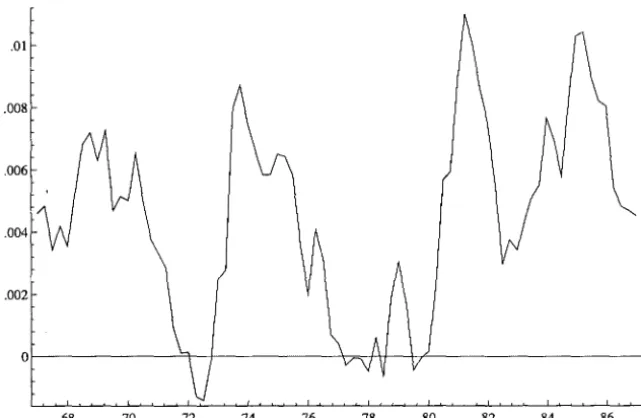
density regions. Figure 2.2 presents the posterior densities of each element of a, which are skewed and lie far from zero. Figure 2.3 plots the cointegration relationship, which shows slightly upward trending.

The over-identifying restriction on the cointegrating vector is tested com-puting the Bayes factors using (2.25) and (2.23). The computed Bayes fac-tors are 138.87 and 97.4 respectively. Therefore, there is strong evidence to support the consumption-income relation (see the guideline in Table 1.1,

Figure 2.1: Posterior Density of f3 for the 'Great Ratios'

Posterior density of b I

[ bli 2

Poste~6r density -lfb2

2.5 ,.---;::;-,

~-b2

2

1.5

.5

-3.5 -3 -2.5 -1.5

-2

-1 -.5 o .5 1.5

-1.5 -1 -.5 o .5

Figure 2.2: Posterior Density of a for the 'Great Ratios'

Posterior density of alphal

l

"I

~

, I ! • ~

- 05 -.025 0 .025 .~5

r:~~rd<m'"

" ...

.075 .1 .125 .15 .175 .2 .225 .25 .275 .3

-.1 -05 .0 .05 .1

Posterior denSIty of alpha3

r=~

.15 .2 .25 .3 .35 .4 .45 .5 .55

..

,J j

AI1L

-.025 0 .025 .05 .075 .1 .125 .15 .175 .2 .225 .25 .275 .3 .325 1.5

.325

.6

[image:50.572.114.430.167.384.2]

Figure 2.3: Cointegration Relationship for the 'Great Ratios'

.01

.008

.002

[image:51.567.106.427.173.382.2]

2.6.2

Cointegration Test for PPP and VIP

Johansen and Juselius (JJ) (1992) studied cointegration for UK's PPP and UIP hypotheses by using likelihood ratio tests. In this subsection PPP and UIP hypotheses are tested by the various Bayesian method. The data are quarterly and have the following five variables: P (log of UK wholesale price), P F (log of trade weighted foreign wholesale price), R (three-month treasury bill rate in the UK), RF(three-month Eurodollar interest rate), E (log of UK effective exchange rate). As JJ conditioned their model on changes in oil prices and quarterly seasonal dummies, DPO (changes in real oil prices),

DPO(-l) (changes in real oil prices with one lag), and SI, S2, S3 (quarterly

seasonal dummies) are also included in the model as exogenous variables. The sample period is 1972(1) to 1987(2) with 62 observations. The VAR model for

Yt

= _{[Pt RFt P}

Ft

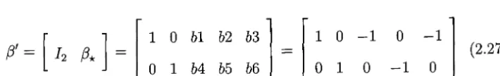
_{R t Et]} I is with 2 lags (chosen by SBIC) and an

intercept term. Bayesian models are constructed with the same manner as the prior specifications in the previous example. Long-run economic theory suggests that two cointegrating vectors are expected as:

,_ [ ] _ [ l O b I b2 b3] =

[1

0

-1

f3 -

12

f3*

-o

1 b4 b5 b6 0 1 0

o

-1

-1]

o

(2.27)

The first rows of (2.27) represents the PPP relation and the second is the UIP relation.

[image:52.567.98.453.511.565.2]

test, the trace test rejects the null of r ~ 1 against the alternative of r

?::

2 and cannot reject the null of r ~ 2 against r

?::

3 with 5 per cent significant level, suggesting r

=

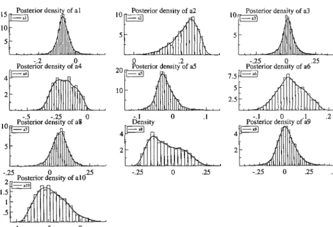
2.

Table 2.8 reports the posterior means and standard deviations for each unrestricted element of (3 and a estimated by Bayesian method proposed in previous section. Figure 2.4 and 2.5 plot the posterior densities of the cointegrating vector (3* and the adjustment term a. The first five densities of a (al a5) correspond to the first cointegrating vector and the rest (a6 -al0) to the second cointegrating vector.

Table 2.7: Cointegration Tests for PPP and UIP: Posterior Probabilities

I

rank r

I

PlC

0 -7.183 0.000 0.066 0.088 1 -0.737 0.033 0.831 0.385 2 -0.755 0.580 0.103 0.513 3 -0.712 0.387 0.000 0.014 4 -0.693 0.000 0.000 0.000 5 -0.710 0.000 0.000 0.000 Note:

PlC: Posterior Information Criterion

Kpl: Kleibergen and Paap method with 9 = 1.00 KP2: Kleibergen and Paap method with 9 = 0.01 Kp3 : Kleibergen and Paap method with diffuse prior Bpl: uses the Schwarz BIC given in (2.25)

BP2: uses the harmonic mean of the likelihood given in (2.23)

Johansen: the numbers are p-values by Johansen's trace test

BF2 Johansen I

0.101 0.013 0.004** 0.111 0.094 0.034* 0.788 0.893 0.058 0.000 0.000 0.176 0.000 0.000 0.023 0.000 0.000

-Table 2.8: Posterior Results of (3* and a (,\

=

1.00) for PPP and UIP Mean s.d

Mean s.d Mean s.d

(3*1 -1.139 0.053 _{-0.066 0.031 0.042 0.054} (3*2 -3.712 1.191

al a6

a2 0.217 0.052 a7 0.058 0.056

(3*3 -0.545 0.118 _{a3 0.015 0.058 as -0.005 0.115} (3*4 -0.074 0.010

a4 -0.193 0.085 ag 0.022 0.091

(3*5 -0.590 0.323 _{-0.022 0.028 -0.442 0.219} (3*6 0.154 0.027

[image:54.564.108.432.155.259.2]

[image:55.566.102.440.179.405.2]

Figure 2.4: Posterior Densities of (3 for the PPP & DIP

Density

3 1-Posterior desilY of b II

2

1.0

0.5

-1.75 -1.50 -1.25 -1.00 -0.75 -0.50 Density

-1.5 -1.0 -0.5 0.5

Density

1.0 1-Posterior desity of bsl 0.5

-4 -3 -2 -1

1.0 0.50

0.25

-5 -4 -3 -2 -1

Density

1-Posterior desity of b41

5.0

2.5

-0.50 -0.25 0.00 0.25 4 _1-Density

Posterior desity of b61n

3 ! !

2

-0.50 -0.25 0.00 0.25 0.50

o

0.50

Figure 2.5: Posterior Densities of a for the PPP & DIP

::r"~I

-.2 0

Posterior density of a4

4 I .1\ ~ '1

2

-.25 0 .25

::~

-.5 -.25 0

't~~][.

:rI

-.I 0 .1 .2

-.25 0 .25

2~p~~:eri~r~nSity ofalO

1.5 . .

'1

1 i

.5

!

I

-.25 o .25 -.25 o .25 .5

[image:56.564.102.438.174.403.2]

Figure 2.6: Cointegration Relationships for the PPP & UIP

.08 1st cointegration relation

.07

.06

.05

.04

.115

.11

.105

1972 1973 1974 1975 1976 1977 1978 1979 1980 1981 1982 1983 1984 1985 1986 1987 1988 2nd comtegration relation

Table 2.9: Over-Identifying Restrictions on {3: values of Bayes Factors for PPP and DIP

Restrictions Test

{3'

=

r

1 0

_o

-1 0

~1

_J

PPP 0.131 0.022 1

_{* *}

{3'

=

r

1 0

*

0 1 0 -1 0

* *

J

DIP 743.8 108.4 {3'

=

11 0 -1 0

~1

_J

_{PPP&DIP 0.001 0.0003}

o

1 0 -1

[image:57.570.105.430.156.377.2] [image:57.570.125.415.464.564.2]

2.7 Conclusion

This chapter introduced a simple method of Bayesian cointegration analysis, and compares this method with other Bayesian methods such as the PlC and the KP method. The Bayes factors are used for computing the poste-rior probabilities for each rank using approximation method with Schwarz BIC and the harmonic mean of the likelihood, which provide insensitive in the choice of the prior parameters. Monte Carlo simulations show that the Bayes factors computed by using the harmonic mean of the likelihood tend to select the correct cointegrating rank than those by using the Schwarz BIC approximation method when the sample size is small. However, when the sample size is large, the Bayes factors approximated by the SBC performs slightly better. The Bayes factors are also applied to test over-identifying restrictions on the cointegrating vectors.

For the comparison with the PlC, we find that the performance of the PlC depends upon the sample size as we expected. In the Monte Carlo experiments, the PlC shows better performance when the true rank is 0 or 1, however, the performance is much worse when the true rank is higher. With large sample size, the PlC shows the best performance among others.

Markov Switching Cointegration

Model

3.1

Introduction

The previous chapter deals with a linear cointegration model with a Bayesian approach. This chapter introduces a Markov switching cointegration model that allows the cointegration relationships to be switched on and off depend-ing on the regime, and its application to purchasdepend-ing power parity (PPP). We also present a cointegration model in which deviations from the long-run equilibrium are characterised different rates of adjustment depending on the regime. Many economic theories are concerned with equilibrium relationships in which several series are expected to be cointegrated each other. However, it is sometimes not possible to find such cointegrating relationships because of presence of transaction costs, adjustment costs, or government's policy change. Especially in the goods market disequilibria may take a considerable

amount of time to be reversed (Brenner and Kroner, 1995). There are several statistical explanations for failing to reject the null of no cointegration due to the span of the data set (Hendry, 1995), structural breaks (Gregory and Hansen, 1996, and Campos, et al., 1996), and the choice of the number of lags in the VAR (Banerjee, et al., 1993).

error correction model for signs of Markov switching behaviour. That is, after finding the cointegration relation

f3

based on the linear cointegration model, set up the cointegration relationships

f3'

Xt = Zt and then investigate

whether

{Zt}

follows a threshold process with one stationary, and one non-stationary regime. This two-step method1 _{is asymptotically valid but might}

yield unreliable estimation for cointegrating vectors when the sample size is small and/or when a regime where cointegration is present is not dominant over the sample period. Suppose we analyse Markov switching VECM such

as ~Yt

=

a St f3'rnYt-1

+

et where the state variable 8t takes 1 if cointegration

is present and 0 if not; a st=l = a1

#-

0 and aSt=O = O. The cointegrat-ing vector, f3NL, might be exactly estimated by modeling linear cointegrated VECM ~Yt

=

af3~Yt-1

+

et if enough large observations for a regime when cointegration is present are available in the Markov switching cointegration model. However, if only a small sample size is available, estimated

(3L

will be largely biased from the true f3NL. Thus, a classical method such as Balke and Fomby could be misleading. There might be a method that can estimate f3NL

directly within the nonlinear models in classical framework such as using a grid search method. However, it will not be easy. To overcome this problem, we employ a Bayesian method with Markov Chain Monte Carlo (MCMC) simulation techniques to estimate parameters such as f3NL conditional on the estimated set of regime variables S

=

{81' 82, . . . ,

8T}'

in each iteration of the

Gibbs sampler so that we can obtain more accurate estimated values of f3NL'

In Markov switching models, some parameters are dependent on an

observed regime variable St that is an outcome of discrete Markov process. In

the classical methods, inference on the unobserved Markov switching variable S

=

{SI,

S2,···, ST}' is made on the conditional distribution after making

in-ferences on the model's unknown parameters. In Bayesian method, both the parameters of the model and the regime variables S are treated as random variables, and thus inference on S is based on a joint distribution.

Applying a Bayesian approach has another advantage for a nonlinear cointegration model. Bayes factors enable to test for a no-cointegrated lin-ear model against Markov switching cointegration models, while in classical methods it is difficult to test because of nonstandard inference problem due to the presence of unit roots and the unidentifiability of the nuisance parame-ters under the null hypothesis. By taking this advantage of the Bayes factors, we can select the most appropriate model among more various models under consideration.

is significantly different from the estimated i3NL by the Bayesian Markov

switching cointegration model with the posterior distribution for i3NL

condi-tional on the regime variables. Section 3.5 contains concluding remarks and suggestions for future work.

3.2 Bayesian Estimation of the Markov

Switch-ing Cointegration Model

3.2.1 Markov Switching Cointegration Model with

Two-Regime

This section proposes a Markov switching cointegration model. Let Xt

de-note an 1(1) vector of n-dimensional time series with r linear cointegrating relations. The long-run multiplier matrix is IT

=

On when the regime vari-able, St, takes its value zero, and IT

=J

On when St

=

1. If we assume that the

intercept term J.l in Gaussian VAR is also subject to Markov switching, then the VECM representation is:

p-l

I:l.Xt = J.lSt

+

ITStXt-1

+

2:

Wil:l.Xt-i

+

et i=l

(3.1)

where t

=

p,p

+

1, ... , T, and p is the number of lags, and the errors et are assumed N(O,~) and independent over time. Dimensions of matrices are J.l

and e (n x 1), IT, W and ~ (n x n). The state variable St evolves