The Minimal Preprocessing Pipelines for the Human
Connectome Project
Matthew F. Glassera, Stamatios N Sotiropoulosb, J Anthony Wilsonc, Timothy S Coalsona,
Bruce Fischld,e, Jesper L Anderssonb, Junqian Xuf,g, Saad Jbabdib, Matthew Websterb,
Jonathan R Polimenid, David C Van Essena, Mark Jenkinsonb, and for the WU-Minn HCP Consortium
Stamatios N Sotiropoulos: [email protected]; J Anthony Wilson: [email protected]; Timothy S Coalson: [email protected]; Bruce Fischl: [email protected]; Jesper L Andersson: [email protected]; Junqian Xu: [email protected]; Saad Jbabdi: [email protected]; Matthew Webster: [email protected]; Jonathan R Polimeni: [email protected]; David C Van Essen: [email protected]; Mark Jenkinson:
aDepartment of Anatomy and Neurobiology, Washington University Medical School, 660 S. Euclid
Avenue, St. Louis, MO 63110, USA
bCentre for Functional Magnetic Resonance Imaging of the Brain (FMRIB), University of Oxford,
Oxford, UK
cMallinckrodt Institute of Radiology, Washington University Medical School
dAthinoula A Martinos Center for Biomedical Imaging, Department of Radiology, Harvard Medical
School/Mass. General Hospital, Boston, MA, USA
eComputer Science and AI Lab, Mass. Institute of Technology, Cambridge, MA
fCenter for Magnetic Resonance Research, University of Minnesota Medical School, Minneapolis,
Minnesota, USA
gTranslational and Molecular Imaging Institute, Icahn School of Medicine at Mount Sinai, New
York, NY, USA
Abstract
The Human Connectome Project (HCP) faces the challenging task of bringing multiple magnetic resonance imaging (MRI) modalities together in a common automated preprocessing framework across a large cohort of subjects. The MRI data acquired by the HCP differ in many ways from data acquired on conventional 3 Tesla scanners and often require newly developed preprocessing methods. We describe the minimal preprocessing pipelines for structural, functional, and diffusion MRI that were developed by the HCP to accomplish many low level tasks, including spatial artifact/distortion removal, surface generation, cross-modal registration, and alignment to standard space. These pipelines are specially designed to capitalize on the high quality data offered by the HCP. The final standard space makes use of a recently introduced CIFTI file format and the associated grayordinates spatial coordinate system. This allows for combined cortical surface and subcortical volume analyses while reducing the storage and processing requirements for high
© 2013 Elsevier Inc. All rights reserved.
First Author/ Corresponding Author Matthew F. Glasser, +1-404-247-1694 (tel), +1-314-747-3436 (fax),
Publisher's Disclaimer: This is a PDF file of an unedited manuscript that has been accepted for publication. As a service to our
customers we are providing this early version of the manuscript. The manuscript will undergo copyediting, typesetting, and review of
NIH Public Access
Author Manuscript
Neuroimage
. Author manuscript; available in PMC 2014 October 15.Published in final edited form as:
Neuroimage. 2013 October 15; 80: 105–124. doi:10.1016/j.neuroimage.2013.04.127.
NIH-PA Author Manuscript
NIH-PA Author Manuscript
spatial and temporal resolution data. Here, we provide the minimum image acquisition
requirements for the HCP minimal preprocessing pipelines and additional advice for investigators interested in replicating the HCP’s acquisition protocols or using these pipelines. Finally, we discuss some potential future improvements for the pipelines.
Keywords
Human Connectome Project; Image Analysis Pipeline; Surface-based Analysis; CIFTI; Grayordinates; Multi-modal Data Integration
Introduction and Rationale
The Washington University-University of Minnesota Human Connectome Project
Consortium (WU-Minn HCP) (Van Essen et al., 2012a) is charged with bringing data from the major MRI neuroimaging modalities, structural, functional, and diffusion, together into a cohesive framework to enable cross-subject comparisons and multi-modal analysis of brain architecture, connectivity, and function. Specifically, the imaging modalities include T1-weighted (T1w) and T2-T1-weighted (T2w) structural scans, resting-state and task-based functional MRI scans, and diffusion-weighted MRI scans. Additionally, the HCP is committed to making these complex datasets publicly available and easy to use. Although the HCP will make the unprocessed NIFTI data available for all usable scans, we anticipate that many investigators will prefer to use the outputs of the minimal preprocessing pipelines, developed by members of the WU-Minn HCP in collaboration with members of the MGH/ UCLA HCP. Investigators in the HCP consortia have acquired extensive experience with the state-of-the-art imaging data being generated by the HCP though their involvement in the 2-year-long piloting phase (I). The WU-Minn HCP Phase II data are being acquired on a customized Siemens Skyra 3T scanner, using advanced pulse sequences that are described elsewhere in this special issue (Ugurbil et al.; Smith et al.; Sotiropoulos it et al., THIS ISSUE). Many of the HCP datasets are qualitatively different from standard neuroimaging data, having higher spatial and temporal resolutions and differing distortions. As a result, these data must be processed differently to achieve optimal results. Users of unprocessed data must deal with complex and esoteric issues that are particularly relevant for these acquisitions, such as the correction of gradient nonlinearity distortion in images that were acquired with oblique slices relative to the scanner’s coordinate system. These and many other preprocessing considerations have already been resolved in the minimally
preprocessed data. Additionally, the minimal preprocessing pipelines include steps, such as field map distortion correction, which are widely accepted to be beneficial (Cusack et al., 2003; Jezzard and Balaban, 1995) but often neglected in practice. Finally, the minimal preprocessing results are available in standard volume and combined surface and volume spaces to enable easier comparisons across different studies, both within the HCP
consortium and outside of it. By taking care of the necessary spatial preprocessing once in a standardized fashion, rather than expecting each community user to repeat this processing, the minimal preprocessing pipelines will both avoid duplicate effort and ensure a minimum standard of data quality. Moreover, for users working with HCP data, the preprocessing pipelines will make it easier to report findings in a common space and replicate analytic efforts. We anticipate that most investigators will be more interested in the analyses that they can do with the HCP data, and less interested in repeating or refining the complicated preprocessing required to best capitalize on these cutting edge data.
The overall goals of the six minimal preprocessing pipelines are 1) to remove spatial artifacts and distortions; 2) to generate cortical surfaces, segmentations, and myelin maps; 3) to make the data easily viewable in the Connectome Workbench visualization software
NIH-PA Author Manuscript
NIH-PA Author Manuscript
(Marcus et al, THIS ISSUE); 4) to generate precise within-subject cross-modal registrations; 5) to handle surface and volume cross-subject registrations to standard volume and surface spaces; and 6) to make the data available in the CIFTI format in a standard “grayordinates” space (see below). While achieving these goals, the minimal preprocessing pipelines are designed to minimize the amount of information actually removed from the data. Further preprocessing, such as, significant spatial smoothing, temporal filtering, nuisance regression, or motion censoring (scrubbing), all remove significant amounts of information. Moreover, the preferred strategies for using these techniques remain subjects of debate (Carp, 2011; Fox et al., 2009; Murphy et al., 2009; Power et al., 2011, 2012; Saad et al., 2012; Turner, 2012). Thus, these forms of preprocessing fall outside the scope of “minimal preprocessing,” and are largely covered elsewhere (e.g. Smith et al. THIS ISSUE, Barch et al THIS ISSUE). While the HCP consortium may make some choices and suggestions on these steps that remove information, many investigators will presumably prefer to make different choices. Additionally, there is no consensus as to the best way to analyze these imaging modalities after preprocessing, and new analysis methods will continue to be developed. Thus, while the HCP will provide data that have undergone additional analyses, we expect many users will be interested in downloading the minimally preprocessed data as the starting point for their own analyses.
The CIFTI File Format and Grayordinates, a Combined Cortical Surface and
Subcortical Volume Coordinate System
Standard volume-based neuroimaging analyses will be easy to carry out using the outputs of the minimal preprocessing pipelines (e.g. Barch et al THIS ISSUE). However, we note that such analyses will waste many of the potential benefits offered by the high resolution HCP data for greater accuracy in spatial localization, both within individuals and across subject groups. It is now well established (Anticevic et al., 2008; Fischl et al., 2008; Frost and Goebel, 2012; Tucholka et al., 2012; Van Essen et al., 2012b) (Smith et al THIS ISSUE) that it is beneficial to analyze cortical neuroimaging data with surface-constrained methods. The fundamental reason is that the convoluted cortical sheet is most easily manipulated and analyzed as a 2D surface. 2D geodesic distances along the surface, rather than 3D Euclidean distances within the volume, are most neurobiologically relevant in many circumstances and are most suited to the geometry of the cerebral cortex. This insight has important
consequences for image processing, especially spatial smoothing and intersubject
registration. For example, cortical areas are spaced farther apart across the surface than they are in the volume because of the cortical convolutions. Functionally distinct areas may be separated by only a few millimeters in the volume across sulcal banks or gyral blades. Therefore, spatial smoothing constrained to the cortical surface will not mix signals from distinct cortical areas as much as 3D volumetric smoothing—not to mention avoiding mixing in nuisance signals from CSF or white matter (Jo et al., 2007). Additionally, surface-based intersubject registration needs only to align data within the plane of the surface (2D), whereas volume-based intersubject registration must also attempt to align the plane of the surface itself (3D). Thus, surface-based alignment of data across subjects is a somewhat easier problem to solve and yields results that achieve greater overlap (Anticevic et al., 2008; Fischl et al., 2008; Fischl et al., 1999b; Frost and Goebel, 2012; Tucholka et al., 2012; Van Essen et al., 2012b).
In contrast to cortical data, subcortical data generally come from deep grey matter structures and nuclei that exhibit 3D geometry, which is different from the 2D cerebral cortical sheet whose thickness varies only modestly. (Note: the cortical thickness of the cerebellum is much less than that of the cerebral cortex. It cannot be automatically segmented using the pipelines presented here, but in the future, new methods may be able to perform cerebellar surface reconstruction with the high-resolution HCP datasets. For now the cerebellum is
NIH-PA Author Manuscript
NIH-PA Author Manuscript
treated as a volumetric structure, but future surface-based analysis of the cerebellum is supported within the existing CIFTI file format, Connectome Workbench, and its commandline algorithms). 3D subcortical structures are best analyzed in 3D volumetric space, both with regard to spatial smoothing and to cross subject comparisons. We use FreeSurfer to automatically segment many subcortical grey matter structures (Fischl et al., 2002). Much like we constrain cortical grey matter analyses to the surface, we can limit subcortical grey matter analyses to these automatically segmented parcels in each individual. We can then constrain 3D volumetric spatial smoothing to occur only within parcel
boundaries, for example avoiding mixing signals from the third ventricle into the medial thalamus. Such parcel-constrained volumetric smoothing should in principle reduce the amount of noise being mixed into the grey matter structures of interest. Additionally, while nonlinear volume registration does an excellent job of aligning subcortical parcels
(Andersson et al., 2007; Klein et al., 2009), we can constrain cross-subject comparisons of subcortical data to occur only within the subcortical parcels of each subject. This precise correspondence is achieved by resampling the sets of voxels in each of the subjects’ individually defined subcortical parcels to a standard set of voxels in each atlas parcel (see fMRISurface Pipeline below).
The Connectivity Informatics Technology Initiative (CIFTI) file format was created to support a variety of connectome-specific data representations, including combinations of cortical grey matter data modeled on surfaces and subcortical grey matter data modeled in volumetric parcels (http://www.nitrc.org/plugins/mwiki/index.php/
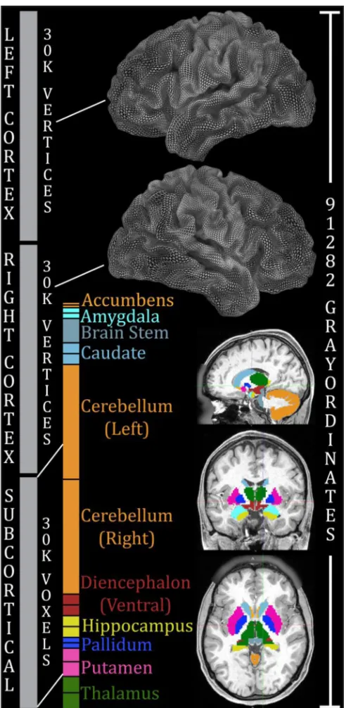
cifti:ConnectivityMatrixFileFormats). Because gray matter can be modeled as either cortical surface vertices or subcortical voxels, the more general term “grayordinates” is used to describe the spatial dimension in this combined coordinate system. When right and left standard cortical surface meshes and a set of standard subcortical volume parcels are used to create a CIFTI grayordinates space, it is said to be a standard grayordinates space (Figure 1). Such a standard CIFTI grayordinates space has more precise spatial correspondence across subjects than volumetrically aligned data and is the desired endpoint of the HCP minimal preprocessing functional pipelines. The HCP rfMRI and tfMRI timeseries data are provided in this space (and also as NIFTI files in MNI volume space).
CIFTI was also developed to enable a more compact representation of high spatial and temporal resolution MRI data. Generation of a Dense Connectome (a matrix describing the connectivity from each grey matter point to all other grey matter points) is one instructive example. Early on in the HCP we realized that the generation of such a matrix would be to be extremely memory intensive and would require huge storage capacity. For example, the 2mm MNI space brain mask distributed with FSL (Smith et al., 2004) contains 228,483 voxels. A dense connectome with this spatial dimension would need 228,483 × 228,483 × 4bytes = ~195GB per modality, per analysis method, per subject. A key insight was the realization that all of grey matter could be represented at a 2mm resolution using only 91,282 grayordinates (Figure 1), including ~30,000 surface vertices (average inter-vertex spacing of 2mm) for each hemisphere and ~30,000 2mm subcortical grey matter voxels producing a CIFTI dense Connectome = 91,282 × 91,282 × 4bytes = 31GB. Combining only surface and volume grey matter data saves 84% of the space while still representing all of the grey matter to grey matter connectivity at the original 2mm resolution. Similarly for a single 1200 timepoint resting state run (14.4 minutes at 720ms TR), the CIFTI dense timeseries, consisting of grayordinates by time is 91,282 × 1200 = 0.41GB versus 228,483 × 1200 = 1.02GB for the masked volume timeseries, saving 60% of the space. The benefits are even larger when one considers that rectangular NIFTI volumes are often not masked at all in memory, storing many voxels outside the brainmask, and the same resting state run unmasked is 104 × 90 × 72 × 1200 = 3.01GB, with a CIFTI dense timeseries now providing an 86% savings in uncompressed disk space and, more importantly, memory. Thus, the
NIH-PA Author Manuscript
NIH-PA Author Manuscript
CIFTI file format is important for reducing the computational and storage demands of high spatial and temporal resolution data. These considerations will only grow in importance as imaging resolutions continue to increase (e.g. with higher field strength). CIFTI also combines the left and right cerebral hemispheres and subcortical parcels into a single file, thereby simplifying file management for combined surface and volume analyses and visualization.
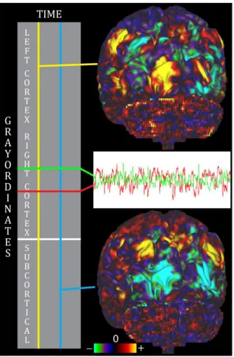
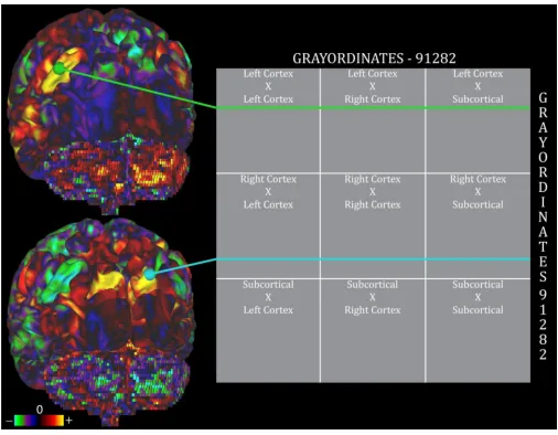
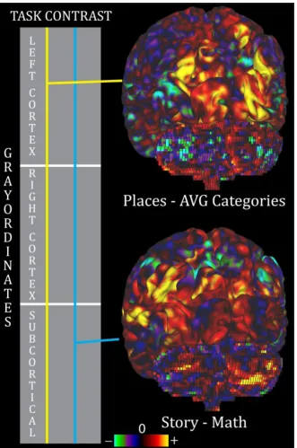
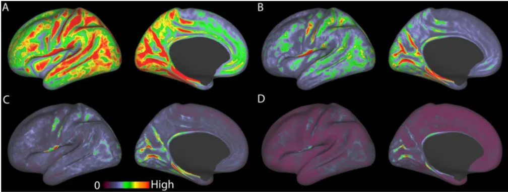
CIFTI files contain a single 2D matrix. One dimension of the matrix always represents the spatial domain (often the standard set of grayordinates) and the other dimension may represent something else. For instance, in the dense timeseries file type, the rows represent the spatial dimension, and the columns represent timepoints (Figure 2). In the dense Connectome file type, both matrix dimensions are spatial (grayordinates) (Figure 3). It is also possible to represent other types of data in grayordinates space, including ICA
component spatial maps or task fMRI z-statistic contrast maps (Figure 4) in dense scalar file, or parcellation labels in a dense label file. A CIFTI file can be valid even if it contains only surface data from just one cerebral hemisphere, or the cerebellum, or just volume data. Within the HCP’s standard CIFTI grayordinates space, datasets from different subjects have the same spatial dimension, allowing straightforward grayordinate-wise comparisons across subjects. For the HCP data, these spatial correspondences have been achieved separately using the registration methods best suited to aligning each domain, i.e., nonlinear surface registration for the cortical structures and nonlinear volume registration for the volume structures (see HCP Structural Pipelines below).
Although the cortical surface and subcortical volume data are stored in a single 2D matrix, the CIFTI header contains information describing the structure that each row and column of the matrix belong to. For example, inside the HCP’s 2mm standard grayordinates space, row 1000 of the matrix would correspond to vertex 2152 of the left hemisphere surface (not vertex 1000, because vertices in the medial wall are excluded) and row 91000 would correspond to voxel (3.9,−1.4, 10.6) of the right thalamus. CIFTI files may contain whatever space the user chooses, however. Connectome Workbench (Marcus et al THIS ISSUE), the surface and volume data visualization platform customized for HCP data, can use the information in the CIFTI header to display the contents of the data matrix on the correct structures and in the correct spatial locations, as illustrated in Figures 2–4.
CIFTI is a new file format that is currently only supported natively by Connectome
Workbench and its commandline utilities. While we encourage other neuroimaging software platforms to implement CIFTI compatibility, there are a variety of ways that these
neuroimaging platforms can already make use of CIFTI data, benefiting from existing Connectome Workbench commandline file conversion utilities. If users need only to perform an analysis that treats each grayordinate independently, without reference to the spatial relationships between grayordinates, one can convert a CIFTI file to a NIFTI-1 file (by wrapping the grayordinates spatial dimension into the volumetric x, y, and z dimensions and keeping time as the 4th NIFTI-1 dimension). Examples where this is useful include ICA analysis of a CIFTI dense timeseries in FSL’s melodic, or element-wise task fMRI analyses with FSL’s contrast_mgr or flameo executables. Similarly for generic analyses, CIFTI files can be converted to GIFTI external binary files for reading into Matlab. If knowledge of the spatial relationships needs to be preserved in the external software (an example is FSL’s film_gls tool for task fMRI analysis), a CIFTI file can be split into GIFTI surface data and NIFTI volume data, analyzed in separate parts, and then recombined into a CIFTI file. Finally, in Connectome Workbench’s commandline utilities we have prioritized developing CIFTI compatible algorithms that require knowledge of the spatial relationships in
grayordinates data, such as spatial smoothing and resampling from one CIFTI standard space to another. We also provide flexible math commands that can be used evaluate
NIH-PA Author Manuscript
NIH-PA Author Manuscript
mathematical expressions on CIFTI files. FSL is expected to include full CIFTI support in the future, but will provide surface analysis support via GIFTI files in the short-term (e.g. Barch et al THIS ISSUE).
During the piloting phase of the HCP grant (first two years) both acquisition (Ugurbil et al THIS ISSUE) and preprocessing methods were improved. One of these improvements was to incorporate preprocessing steps that capitalize on the advantages of CIFTI grayordinates datasets. In particular, we avoid unconstrained volume-based smoothing and cross subject averaging, instead using the more constrained methods described above. These
methodological changes enable analyses that depend critically on accurate spatial localization, for example multi-modal cortical areal parcellation in which one attempts to estimate areal boundaries, measuring the areal extent of task-based activation, or measuring the areal extent resting state functional connectivity (Glasser et al., 2012a; Glasser et al., 2011). More conventional neuroimaging analyses that focus on peak activation coordinates or use spheres of a given radius as connectivity seeds may not require these improvements in spatial localization. Moreover, these methodological improvements reduce the need for spatial smoothing to attempt to account for alignment inaccuracies across subjects in group studies (Turner, 2012). We contend that it is generally better to avoid smoothing group data, in order to retain as much spatial detail as possible, though individual data may need to be smoothed (in a grayordinates-constrained way) to increase the signal/contrast of interest relative to high spatial frequency noise (e.g. myelin maps: (Glasser and Van Essen, 2011)). Continued improvements in cross-subject registration, such as driving registration with maps of properties more directly tied to the locations of cortical areas (e.g. myelin maps, task activations, and/or functional connectivity) (Robinson et al., 2013a; Robinson et al., 2013b) should accentuate this principle of better cross-subject cortical areal alignment, requiring even less spatial smoothing.
The above conceptual improvements in methodology served as guiding principles during the development of the minimal preprocessing pipelines presented here. We chose or developed methods that are fully automated and robust, so that large amounts of data can be processed without user intervention. Additionally, we used methods that cause minimal blurring and achieve accurate cross-modal alignment to enable use cases focused on fine details in the data. This will likely be an ongoing effort throughout the duration of the HCP, as the pipelines presented here will presumably undergo additions and improvements over time (see Future Directions below). Before discussing the pipelines themselves, we describe aspects of the HCP data acquisitions that are relevant to developing or running the HCP minimal preprocessing pipelines, but are not covered elsewhere in this issue (Ugurbil et al. THIS ISSUE; Smith et al. THIS ISSUE; Sotiropoulos et al. THIS ISSUE).
HCP Structural Acquisitions
The HCP structural acquisitions include high resolution T1-weighted (T1w) and T2-weighted (T2w) images (0.7mm isotropic) for the purpose of creating more accurate cortical surfaces and myelin maps than are attainable with lower resolution data (Glasser and Van Essen, 2011). While high spatial resolution was a primary goal, we also optimized the contrast parameters (flip angle (FA) and inversion time (TI) for the T1w scans, and echo time (TE) for the T2w scans). The major change from Glasser and Van Essen (2011) was to lengthen TE in the T2w scans to improve intracortical contrast for myelin detection. Additionally, B0 fieldmaps, B1−, and B1+ maps are acquired for the purpose of correcting
readout distortion in the T1w and T2w images and to enable future correction of intensity inhomogeneity by explicitly modeling the B1− receive and B1+ transmit fields. 32 minutes
are spent acquiring the main T1w and T2w structural images, and 8 minutes are spent acquiring the auxiliary scans on the HCP’s custom 3T Siemens Skyra (Ugurbil et al. THIS
NIH-PA Author Manuscript
NIH-PA Author Manuscript
ISSUE) using a 32-channel head coil. Two separate averages of the T1w image are acquired using the 3D MPRAGE (Mugler 3rd and Brookeman, 1990) sequence with 0.7mm isotropic resolution (FOV=224 mm, matrix=320, 256 sagittal slices in a single slab), TR=2400 ms, TE=2.14 ms, TI=1000 ms, FA=8°, Bandwidth (BW)=210 Hz per pixel, Echo Spacing (ES) =7.6 ms, with a non-selective binomial (1:1) water excitation pulse (a pair of 100 µs hard pulses with 1.2 ms spacing) to reduce signal from bone marrow and scalp fat, phase encoding undersampling factor GRAPPA=2, 10% phase encoding oversampling (anterior -posterior) to avoid nose wrap-around, asymmetric readout (i.e. omitting the initial 20% of the total samples before echo) along superior - inferior direction (z) with dwell time of 7.4 µs (used for readout distortion correction with FSL’s FUGUE (Jenkinson et al., 2012)). Two separate averages of the T2w image are acquired using the variable flip angle turbo spin-echo sequence (Siemens SPACE (Mugler et al., 2000)) with 0.7mm isotropic resolution (same matrix, FOV, and slices as in the T1w), TR=3200 ms, TE=565 ms, BW=744 Hz per pixel, no fat suppression pulse, phase encoding undersampling factor GRAPPA=2, total turbo factor=314 (to be achieved with a combination of turbo factor and slice turbo factor, when available), echo train length of 1105 echoes, 10% phase encoding oversampling (anterior - posterior) to avoid nose wrap-around, readout along superior - inferior direction with dwell time of 2.1µs (for readout distortion correction with FUGUE).
All auxiliary scans are acquired at 2mm isotropic resolution. The B0 fieldmap is acquired by
a dual-echo gradient echo sequence with delta TE=2.46ms. The B1− receive field can be
calculated from proton density weighted images acquired from a FLASH sequence once with the 32 channel head receive coil and once with the body receive coil (similar to Siemens pre-scan normalize). The B1+ transmit field can be calculated from an actual
flip-angle imaging (AFI) acquisition (Yarnykh, 2007) with TR1/TR2 = 20/120ms (target flip angle=50°).
HCP Functional and Diffusion Acquisitions
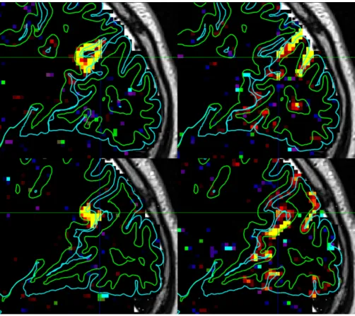
The functional and diffusion acquisitions are described in detail in other papers of this special issue (Ugurbil et al.; Smith et al.; Sotiropoulos et al., THIS ISSUE), but a number of points relevant to the HCP pipelines are noted here as well. The functional data are acquired at 2mm isotropic, which is of unusually high spatial resolution for whole-brain coverage at 3T. Although the spatial specificity of BOLD fluctuations measured at 3T is around 4mm FWHM ((Parkes et al., 2005) Ugurbil et al. THIS ISSUE), there are benefits of sampling the data more finely when the goal is to accurately map grey matter BOLD signals onto the cortical sheet. From a purely geometrical perspective, higher resolution scans provide the potential to decrease induced cross-sulcal and cross-gyral timeseries correlation. Figure 5 uses a simple volume to surface mapping model to illustrate this effect by comparing 4mm, 3mm, 2.5mm, and 2mm fMRI acquisition resolutions and showing that the induced correlations between surface vertices that are far apart across the surface but close together in the volume are mostly eliminated at 2mm isotropic. Thus, with high-resolution data it becomes possible to assign the BOLD signal more specifically to opposing banks of sulci (Figure 6). This effect will become even more beneficial at 7T, where the point-spread-function of the BOLD fluctuations is closer to 2mm FWHM ((Shmuel et al., 2007) Ugurbil et al. THIS ISSUE). Higher resolution also helps limit the partial volume effects of other noise sources such as CSF, large veins, and white matter.
Fast TR sampling using multiband pulse sequences has several benefits (HCP fMRI: TR=720ms, using a multiband factor of 8, FA=52°--reduced from 90° to match the Ernst angle, maximizing SNR). Multiband enables higher spatial resolution acquisitions, requiring large numbers of slices for whole-brain coverage, while still keeping the TR low. It reduces the need for slice timing correction, as all slices in each volume are acquired much closer
NIH-PA Author Manuscript
NIH-PA Author Manuscript
together than in typical fMRI acquisitions (TR ~ 2.5s). Thus, in the HCP pipelines, no slice timing correction is employed. Additionally, it provides more robustness against the effects of rapid head movement, since three volumes are acquired in the time it typically takes to acquire one standard TR volume. A rapid movement may directly corrupt only one of these volumes, potentially leaving two intact, though some motion effects may be more persistent. Fast TR acquisitions require a different strategy for accurate registration to structural data. Because the multiband timeseries images have reduced tissue contrast (due to incomplete T1 relaxation), HCP pipelines use the single-band reference image with full tissue contrast as the image for registration to the structural data.
To reduce the signal loss and distortions from the high-resolution acquisition and to minimize the TE (33ms in our scans) and echo train length, we acquire a balanced number of volumes with left-right and right-left phase encoding directions using an asymmetric acquisition matrix, rather than the more typical anterior-posterior or posterior-anterior phase encoding directions with a symmetric acquisition matrix. The geometrical dimensions of the gradient echo EPI images are 2mm isotropic resolution (FOV: 208mm × 180mm, Matrix: 104 × 90 with 72 slices covering the entire brain). These left-right and right-left phase encoding directions also have the benefit of reducing the chance that the fMRI data would alias in the phase encoding direction or move outside the FOV because of distortion combined with head motion. To more rapidly measure the b0 field for correction EPI distortions, we acquire two spin echo EPI images with reversed phase encoding directions (60 seconds total for 3 pairs of images). (Note that we refer to these images as spin echo fieldmaps, though they measure the field by reversing the phase encoding direction, which is a very different mechanism from standard field maps that use a phase difference calculated from two different TEs). These spin echo EPI images have the same geometrical, echo spacing (0.58ms in our scans), and phase encoding direction parameters as the gradient echo fMRI scans. These images enable accurate correction for spatial distortions in the fMRI images so that these images can be precisely aligned with the structural images. Two of these spin echo EPI fieldmapping pairs are acquired in each functional session, for added robustness with respect to acquisition errors and subject movement, along with one set of B1− receive field-mapping images (with identical parameters to those described in the
structural session).
While the diffusion acquisition is covered in detail in (Ugurbil et al.; Sotiropoulos it et al., THIS ISSUE), a few points deserve mention here. Very high-resolution acquisitions (1.25mm isotropic) were chosen, as this will be critical for accurately mapping connectivity between cortical grey matter regions, as opposed to just localizing major fascicles in deep white matter. To obtain these high-resolution images, it was beneficial (in terms of TE) to use a Stejskal-Tanner (monopolar) diffusion-encoding scheme. This encoding scheme, together with the customized 100 mT/m gradient set in the HCP’s Skyra, achieves sufficient SNR at 1.25mm isotropic resolution and a diffusion-weighting of up to b=3000 s/mm2
(Sotiropoulos it et al., THIS ISSUE). However, the use of a monopolar Stejskal-Tanner diffusion scheme and the more powerful gradients increases eddy current-induced distortions, which require the use of a sophisticated approach for correction (Andersson et al., 2012), (Sotiropoulos et al., THIS ISSUE). Correction for EPI and eddy-current-induced distortions in the diffusion data is based on manipulation of the acquisitions so that a given distortion manifests itself differently in different images (Andersson et al., 2003). Two phase-encoding direction-reversed images for each diffusion direction are acquired. To ensure better correspondence between the phase-encoding reversed pairs, the whole set of diffusion-weighted (DW) volumes is acquired in six separate series. These series are grouped into three pairs, and within each pair the two series contain the same DW directions but with reversed phase-encoding (i.e. a series of Mi DW volumes with RL phase-encoding
is followed by a series of Mi volumes with LR phase-encoding, i=[1,2,3]). These
diffusion-NIH-PA Author Manuscript
NIH-PA Author Manuscript
weighted images are corrected for B0 and eddy current distortions as described in the
diffusion preprocessing pipeline below. In addition to the diffusion-weighted images, one set of B1− receive fieldmapping images, with identical parameters to those described in the
structural session, is acquired.
HCP Pipelines: Minimum Acquisition Requirements
A number of investigators have asked questions such as: “How do I acquire data like the HCP?” and “What data do I need in order to use the HCP pipelines?” Though many studies will not require, or be in a position to acquire, data using protocols identical to those in the HCP, it is worth describing the minimum acquisition requirements for the HCP pipelines, along with suggestions for best acquisition practices. For all of the following, a 32-channel head coil will be very beneficial in providing the SNR necessary to emulate HCP scanning parameters. For the structural pipelines (upon which the functional and diffusion pipelines depend), high-resolution T1w and T2w scans are both required for surface reconstruction. While 1mm isotropic is acceptable, higher resolutions (0.8mm or 0.7mm) appreciably improve surface reconstructions and myelin maps ((Glasser et al., In Press), see below), particularly in thin regions of cortex or regions with thin gyral blades of white matter (e.g. primary somatosensory cortex or early visual cortex, see Figure 13). The T2w image is required to make accurate pial surfaces that exclude dura and blood vessels, which are isointense to grey matter in the T1w image (Figure 14). The T2w image is also used to make myelin maps based on the T1w/T2w ratio (Glasser and Van Essen, 2011). A regular gradient echo fieldmap (magnitude and phase difference) of relatively high resolution (e.g. 2mm isotropic) is recommended to correct the structural images for readout distortion, which differs between the T1w and T2w images because of their differing readout bandwidth (van der Kouwe et al., 2008). However, in practice the relative distortion between the two images is small (≤1mm) even in high susceptibility regions (e.g. inferior temporal cortex and orbitofrontal cortex). For the T1w image, some degree of fat insensitive excitation (Howarth et al., 2006) is recommended to prevent surface reconstruction errors. Nevertheless, off-resonance fat saturation should be avoided for either the T1w or T2w images to preserve contrast for myelin content by not modifying magnetization transfer effects (Glasser et al., In Press). In addition, vendor implemented receive bias field corrections, like Siemens’s pre-scan normalize, must be matched between the T1w and T2w images (either on for both or off for both).
For the functional pipelines, a fieldmap is required, because any neuroimaging analysis that aims for precise cross-modal registration between functional and structural (or other data modalities) will require EPI distortion correction. In general, either standard gradient echo fieldmaps or spin echo EPI fieldmaps can be acquired, though spin echo EPI field maps can be acquired more quickly with less chance of motion corruption. The geometrical
parameters (FOV, matrix, phase encoding direction, resolution, number of slices) and echo spacing must be matched between the gradient echo EPI fMRI timeseries and the spin echo EPI fieldmaps. A single band reference scan also needs to be saved (as a separate series) together with the multi-band timeseries when using a multi-band sequence to serve as the reference for motion correction and for more accurate EPI to T1w registration. Higher spatial (≤2.5mm) and temporal (≤1s) resolutions are recommended for the reasons discussed above. For resting state fMRI scans, longer contiguous runs are preferable to shorter discontinuous runs, for temporal denoising purposes (Smith et al.; THIS ISSUE).
For the diffusion pipelines, the directions of the diffusion-sensitizing gradients should be distributed across the whole sphere to allow for better correction of eddy-current distortions and subject movement (Sotiropoulos et al., THIS ISSUE). In addition, and for estimating EPI distortions as well, pairs of diffusion-weighted volumes acquired with reversed
phase-NIH-PA Author Manuscript
NIH-PA Author Manuscript
encoding directions are needed. Ideally, all volumes are acquired in phase-encoding reversed pairs, as this further helps in robustly estimating eddy-current distortions, but the minimum requirement is that at least a few (one in theory) b0 pairs are acquired in this way. A Stejskal-Tanner (monopolar) diffusion-encoding scheme with multiband acceleration and phase encoding along the left-right direction are recommended to allow reduction of the TE (more SNR) and TR (for the collection of a larger number of unique diffusion directions (Sotiropoulos it et al., THIS ISSUE)). High spatial resolution (≤1.5mm), larger numbers of unique directions (≥128), and multiple q-space shells with moderately high bmax (e.g. 3000 s/mm2), depending on the employed resolution and the available SNR) will be required to take advantage of improvements in diffusion fiber orientation modeling and tractography that are being generated by the HCP. Investigators using standard Siemens Skyra or Trio equivalent scanners will likely need to sacrifice spatial resolution and/or maximum diffusion weighting to achieve high quality results, as the 100mT/m gradients of the HCP Skyra remain an important contributor to the improved diffusion SNR allowing a 1.25mm isotropic resolution with bmax=3000 s/mm2.
HCP Pipelines
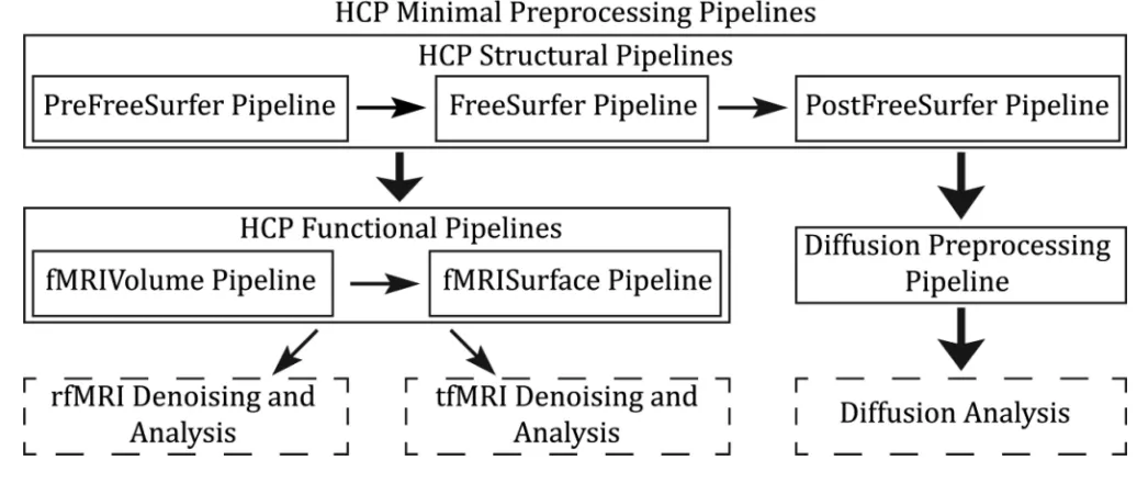
As shown in Figure 7, the six minimal preprocessing pipelines include three structural pipelines (PreFreeSurfer, FreeSurfer, and PostFreeSurfer), two functional pipelines (fMRIVolume and fMRISurface), and a Diffusion Preprocessing pipeline. Figure 7 also shows the overall workflow for preprocessing and data analysis in the HCP. We provide a brief high-level description of all the pipelines, followed by a detailed description of each, including the rationale for choices made in the pipelines and descriptions of novel methods used in them.
HCP Pipelines: Overview
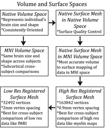
The main goals of the first structural pipeline, PreFreeSurfer, are to produce an undistorted “native” structural volume space for each subject, align the T1w and T2w images, perform a B1 (bias field) correction, and register the subject’s native structural volume space to MNI
space. Thus, there are two volume spaces in HCP data (overview in Figure 8): 1) The subject’s undistorted native volume space (rigidly “aligned” to the axes of MNI space), which is where volumes and areas of structures should be measured and where tractography should be performed, as this space is the best approximation of the subject’s physical brain. 2) Standard MNI space is useful for comparisons across subjects and studies, particularly of subcortical data, which is more accurately aligned by nonlinear volume registration than cortical data is. The FreeSurfer pipeline is based on FreeSurfer version 5.2, with a number of enhancements. The main goals of this pipeline are to segment the volume into predefined structures (including the subcortical parcels used in CIFTI), reconstruct white and pial cortical surfaces, and perform FreeSurfer’s standard folding-based surface registration to their surface atlas (fsaverage). The final structural pipeline, PostFreeSurfer, produces all of the NIFTI volume and GIFTI surface files necessary for viewing the data in Connectome Workbench, along with applying the surface registration (to the Conte69 surface template (Van Essen et al., 2012b)), downsampling registered surfaces for connectivity analysis, creating the final brain mask, and creating myelin maps. There are three surface spaces in HCP data: the native surface mesh for each individual (~136k vertices, most accurate for volume to surface mapping), the high resolution Conte69 registered standard mesh (~164k vertices, appropriate for crosssubject analysis of high resolution data like myelin maps) and the low resolution Conte69 registered standard mesh (~32k vertices, appropriate for cross-subject analysis of low resolution data like fMRI or diffusion). These spaces are also shown in Figure 8. The 91,282 standard grayordinates (CIFTI) space is made up of a standard subcortical segmentation in 2mm MNI space (from the Conte69 subjects) and the 32k
NIH-PA Author Manuscript
NIH-PA Author Manuscript
Conte69 mesh of both hemispheres (Figure 1). Following completion of the structural pipelines, the functional or diffusion pipelines may run.
The first functional pipeline, fMRIVolume, removes spatial distortions, realigns volumes to compensate for subject motion, registers the fMRI data to the structural, reduces the bias field, normalizes the 4D image to a global mean, and masks the data with the final brain mask. Standard volume-based analyses of the fMRI data could proceed from the output of this pipeline. Care is taken in the fMRIVolume pipeline to minimize the smoothing from interpolation, and no overt volume smoothing is done. The main goal of the second functional pipeline, fMRISurface, is to bring the timeseries from the volume into the CIFTI grayordinates standard space. This is accomplished by mapping the voxels within the cortical grey matter ribbon onto the native cortical surface, transforming them according to the surface registration onto the 32k Conte69 mesh, and mapping the set of subcortical grey matter voxels from each subcortical parcel in each individual to a standard set of voxels in each atlas parcel. The result is a standard set of grayordinates in every subject (i.e. the same number in each subject, and with spatial correspondence) with 2mm average surface vertex and subcortical volume voxel spacing. These data are smoothed with surface (novel algorithm, see below) and parcel constrained smoothing of 2mm FWHM to regularize the mapping process. The output of these pipelines is a CIFTI dense timeseries that can be used for subsequent resting-state or task fMRI analyses. The diffusion preprocessing pipeline does the following: normalizes the b0 image intensity across runs; removes EPI distortions, eddy-current-induced distortions, and subject motion; corrects for gradient-nonlinearities; registers the diffusion data with the structural; brings it into 1.25mm structural space; and masks the data with the final brain mask.
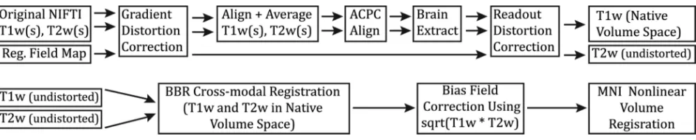
HCP Pipelines: PreFreeSurfer
The PreFreeSurfer pipeline (Figure 9) begins with the correction of MR
gradient-nonlinearity-induced distortions. Because of tradeoffs made in the design of the custom HCP Skyra, the head is ~5cm above isocenter, making the effects of gradient nonlinearities more pronounced in HCP Skyra images relative to those from standard 3T scanners, especially in the frontal lobe (Figure 10). All images used in structural processing (the T1w, T2w, and the field map magnitude and phase) must be corrected for gradient nonlinearity distortion. We did not use the Siemens online gradient distortion correction method because it is not available for all sequences, and the gradient distortion correction must be done on all images for them to align in cross-modal registrations. For the correction of the distortion, the magnetic field generated by each gradient coil is modeled by a spherical harmonic
expansion (specific to the SC72 gradients in the 3T Connectome scanner). The correction is then done with a customized version of the gradient_nonlin_unwarp package available in FreeSurfer (Jovicich et al., 2006). The customized version calculates an FSL-format warpfield that represents the spatial distortion of the image by using a proprietary Siemens gradient coefficient file (available on the scanner used to acquire the images) and the mm coordinate space of the image (including the rotation between image matrix space and scanner axes – that is, the oblique portion of the sform, where the sform is the matrix that relates the voxel coordinates to the mm coordinate space of the scanner, as defined by the NIFTI standard). This warpfield can then either be concatenated with other transforms or applied to the image using spline interpolation (which causes less blurring than trilinear interpolation). While this correction is required for a scanner like the HCP Skyra, which has more significant gradient nonlinearity, it may not be needed for standard scanners (e.g. Siemens Trio) with gradients that are more linear over a larger FOV and where the head position is closer to isocenter. Thus, this correction can be turned off if desired.
NIH-PA Author Manuscript
NIH-PA Author Manuscript
Subsequently, any repeated runs of T1w and T2w images are aligned with a 6 degrees of freedom (DOF) rigid body transformation using FSL’s FLIRT (Jenkinson et al., 2002; Jenkinson and Smith, 2001) and averaged (any number of averages are supported). Note that for the HCP, only T1w and T2w images judged to be “good” or “excellent” in overall quality (quality control procedures described in Marcus et al THIS ISSUE) were used for processing. For many subjects, only a single scan was used for the T1w and/or T2w. For greater robustness, the images are internally cropped to a smaller FOV to remove the neck (150mm in z in humans,) using FSL’s automated robustfov tool, and aligned with a 12 DOF (affine) FLIRT registration to the MNI space templates. This alignment allows the MNI space brain mask to be applied prior to the final registration to mask out any residual shifted scalp fat signal. The final transformation to the output average space is done with spline interpolation to minimize blurring.
Next, the average T1w and T2w images are aligned to the MNI space template (with 0.7mm resolution for the HCP data) using a rigid 6 DOF transform, derived from a 12 DOF affine registration. The 6 DOF transform aligns the AC, the AC-PC line and the inter-hemispheric plane, but maintains the original size and shape of the brain. The goal of this alignment step is to get the images in roughly the same orientation as the template, for convenience of visualization. This step also aligns the coordinate space axes to those of the MNI template, removing any rotation between the mm coordinate space and the image matrix (i.e. it removes the oblique components of the NIFTI sform), as oblique sforms are not consistently handled across imaging software platforms. Similar to the procedure for averaging across runs, robustfov is used to make sure this registration is robust and the transform is applied with spline interpolation. After this “acpc alignment” step, a robust initial brain extraction is performed using an initial linear (FLIRT) and non-linear (FNIRT) registration of the image to the MNI template. This warp is then inverted and the template brain mask is brought back into the acpc-alignment space. We found that this method of bringing the atlas brain mask to the individual’s space outperforms other common brain extraction methods like FSL’s BET (Smith, 2002), albeit at the cost of increased processing time. This initial brain mask is used to assist the final registrations to MNI space and to assist FreeSurfer with its brain mask creation process.
The final step in creating the subject’s undistorted native volume space is removing readout distortion (van der Kouwe et al., 2008), which differs between the T1w and T2w images due to their differing readout dwell times (and thus different bandwidths). This distortion is fairly subtle in comparison to gradient nonlinearity or EPI distortion, but is similar to EPI distortion in that it is greatest in regions with high B0 inhomogeneity due to magnetic
susceptibility differences (orbitofrontal cortex and inferior temporal cortex especially). Thus, readout distortion can be corrected by the same means as EPI distortion, i.e. using a fieldmap as the distortion field and scaling it according to the readout dwell time. For fieldmap preprocessing, a standard gradient echo fieldmap, having two magnitude images (at two different TEs) and a phase difference image, is converted into fieldmap (in units of radians per second) using the fsl_prepare_fieldmap script. Then the mean magnitude and fieldmap images are corrected for gradient nonlinearity distortion (just as for the T1w and T2w images). The fieldmap magnitude image is warped according to the readout distortion and registered, separately, to the T1w and T2w images using 6 DOF FLIRT. The fieldmap is then transformed according to these registrations and used to unwarp the T1w and T2w images, removing the differential readout distortion present in them. Although the T1w and T2w images being corrected are of higher resolution than the field map, the B0
inhomogeneity is smoothly varying and is accurately corrected with this method (see Figure 11). The readout-distortion-corrected T1w image, which now has all spatial distortions removed from it, represents the native volume space for each subject. The undistorted T2w image is cross-modally registered to the T1w image using FLIRT’s boundary-based
NIH-PA Author Manuscript
NIH-PA Author Manuscript
registration (BBR) cost function (Greve and Fischl, 2009) with 6 DOF, bringing it into the native volume space as well. Boundary-based registration seeks to align intensity gradients across tissue boundaries rather than minimizing a cost function over the entire set of image intensities. This registration strategy uses the same contrast mechanism that one uses to evaluate image alignment by eye. If a fieldmap is not available for the structural images, the pipeline has the option to run without it and only perform FLIRT BBR cross-modal
registration of the T2w to the T1w, without removing readout distortion.
Once the T1w and T2w images are in the same space, the same intensity inhomogeneity correction approach used for myelin mapping (Glasser and Van Essen, 2011) is used to correct the T1w and T2w images for B1− bias and some B1+ bias. As described previously
(Rilling et al., 2011), the bias field F is estimated from the square root of the product of the T1w and T2w images after thresholding out non-brain tissues. This method works because the contrast × in the T1w MPRAGE and 1/x in the T2w SPACE within grey and white matter essentially cancel after multiplication, whereas the bias field F does not (Approximation 1).
(1)
After dilating the thresholded bias-field estimate (F) to fill the FOV, the bias field is then smoothed with a sigma of 5mm. This method avoids problems encountered in algorithms like FSL’s FAST (Zhang et al., 2001) and MINC’s nu_correct (Sled et al., 1998) that use white matter homogeneity as the basis for bias field correction. Just as grey matter is inhomogeneous in both T1w and T2w images due to myelin content (Fischl et al., 2004; Glasser and Van Essen, 2011), white matter is also inhomogeneous. Because grey and white matter inhomogeneities are not closely correlated, using inhomogeneities in white matter intensity to correct for those in grey matter is likely to introduce errors (Glasser and Van Essen, 2011).
After bias field correction of the T1w and T2w images, the T1w image is registered to MNI space with a FLIRT 12 DOF affine and then a FNIRT nonlinear registration, producing the final nonlinear volume transformation from the subject’s native volume space to MNI space. The outputs of the PreFreeSurfer pipeline are organized into a folder (by default called T1w) that contains the native volume space images and a second folder (by default called
MNINonLinear) that contains the MNI space images. In addition to working robustly for a number of human datasets (HCP Pilot datasets, Conte69 datasets (Glasser and Van Essen, 2011; Van Essen et al., 2012b), and HCP Phase II datasets), the PreFreeSurfer pipeline also works robustly on chimpanzee and macaque datasets, if given appropriate chimpanzee and macaque templates and brain dimensions (Glasser et al., 2012b). The pipeline is thus not strictly tied to MNI space, and would work with any other standard space, provided that the appropriate template files are generated at the desired output resolution (e.g. the acquired resolution of the data for the high resolution templates).
HCP Pipelines: FreeSurfer
After the PreFreeSurfer pipeline, the FreeSurfer pipeline runs (Figure 12). FreeSurfer’s recon-all pipeline (Dale et al., 1999; Fischl et al., 2001; Fischl et al., 2008; Fischl et al., 2002; Fischl et al., 1999a; Fischl et al., 1999c; Ségonne et al., 2005) is an extensively tested and robust pipeline optimized for 1mm isotropic data; however, we fine-tuned several aspects of this pipeline specifically for the higher resolution HCP Phase II data. A current limitation with recon-all is that it cannot handle images of higher than 1mm isotropic resolution or structural scans of greater than 256 × 256 × 256 voxels. The 0.7mm isotropic
NIH-PA Author Manuscript
NIH-PA Author Manuscript
resolution structural scans we acquire exceed these limits, and must therefore be downsampled to 1mm with spline interpolation prior to launching recon-all. Thus, most processing within recon-all (aside from final surface placement, see below) is conducted in a 1mm isotropic downsampled (RAS) space, which we refer to as FreeSurfer space. The input T1w image to the FreeSurfer pipeline is the native volume space output from the
PreFreeSurfer pipeline—the distortion- and bias-corrected T1w image. This T1w image is normalized to a standard whole brain mean intensity to ensure FreeSurfer’s conversion to an 8-bit datatype is robust. Early on, we found that the HCP Phase II T1w data was not robustly registered using the linear registration within FreeSurfer that precedes FreeSurfer’s brain extraction. This registration is now aided using the initial brain mask generated in PreFreeSurfer to ensure that FreeSurfer’s internal brain mask is correct.
Aside from these changes, FreeSurfer’s recon-all is allowed to run normally, stopping at the point where final white matter surfaces are generated (almost until the end of the autorecon2 step). Important steps that are performed prior this stage include automated segmentation of the T1w volume into a variety of structures (Fischl et al., 2002), plus tessellation and topology correction of the initial white matter surface (Dale et al., 1999). The resultant white matter surface is generated using a segmentation of the 1mm downsampled T1w image. For final white matter surface placement, we make use of the full 0.7mm resolution of the HCP T1w images. The requisite FreeSurfer volume and surface files are brought into the 0.7mm native volume space, the high resolution T1w volume is intensity normalized, and the white matter surface position is adjusted based on intensity gradients in the 0.7mm T1w image. This adjustment corrects for regions in which the white matter surface was placed too superficially in the grey matter because of partial volume effects at 1mm (Figure 13). Additionally, the T2w to T1w registration is fine-tuned using FreeSurfer’s BBRegister algorithm (Greve and Fischl, 2009), which gave slightly more accurate results than FLIRT’s BBR implementation, most likely because of the higher quality surfaces used in the
FreeSurfer BBR registration (the surface used in the PreFreeSurfer pipeline is based on a simple FSL FAST segmentation (Zhang et al., 2001)). The corrected white matter surfaces are then brought back into FreeSurfer space and recon-all processing continues (note that the surfaces are not retessellated so they do not have as many vertices as native 0.7mm images would produce). Spherical inflation of the white matter surface (Fischl et al., 1999a), registration to the fsaverage surface template based on cortical folding patterns (Fischl et al., 1999c), and automated segmentation of sulci and gyri (Desikan et al., 2006) are among the steps done during this recon-all stage.
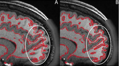
Just before the pial surfaces are generated, recon-all is stopped again and pial surfaces are obtained with an improved algorithm that uses both the high-resolution T1w and T2w images. First, T1w and T2w images are normalized to a standard mean white matter intensity. As noted above, because residual intensity inhomogeneity after PreFreeSurfer bias-field correction is not necessarily correlated between grey and white matter, we do not use the FreeSurfer white matter specific intensity normalized image for pial surface generation. Instead, we carry out a greymatter specific intensity normalization of the T1w image as follows. Initial pial surfaces are generated from the high-resolution PreFreeSurfer bias-field corrected T1w image using relaxed Gaussian parameters (including intensities 4 sigmas above and below the grey matter mean intensity, versus the standard setting of 3 sigmas). This tends to include large amounts of dura and blood vessels (See Figure 14) and may cause the pial surface not to properly follow sulcal fundi, but it reduces the probability of excluding lightly myelinated grey matter. To remove the dura and blood vessels, the pial surface is eroded using the T2w image. Both dura and blood vessels are very different in intensity from grey matter in the T2w image, though they are close to isointense in the T1w image (Figure 14). This initial pial surface is used together with the white matter surface to define an initial grey matter ribbon of voxels whose centers lie between the two surfaces.
NIH-PA Author Manuscript
NIH-PA Author Manuscript
The T1w image is smoothed using a ribbon constrained approach and a sigma of 5mm, and then the original image is divided by this smoothed image (after removing the mean). These operations effectively perform spatial highpass filtering within the grey matter ribbon, removing the low frequency effects of differences in myelin content across the image while keeping the high frequency effects of opposing cortical pial surfaces and radial intracortical contrast. This spatially highpass filtered T1w image is used to regenerate the pial surface from scratch with much more restrictive Gaussian parameters (2 sigmas above and below the grey matter mean intensity). The T2w surface is again used to remove any dura and blood vessels, and the result is the final pial surface. The pial surface now appropriately follows the contours in the volume, but does not exclude lightly myelinated grey matter. The benefits of these operations are evident in the group average Conte69 myelin maps presented previously (Glasser and Van Essen, 2011), especially in the very lightly myelinated medial prefrontal and anterior cingulate cortices (Figure 15). After this pial surface generation step, recon-all then continues to completion. The final steps include surface and volume
anatomical parcellations and morphometric measurements of structure volumes and surface areas.
HCP Pipelines: PostFreeSurfer
The first task of the PostFreeSurfer pipeline (Figure 16) is to take the outputs of FreeSurfer that are in FreeSurfer proprietary formats and convert them to standard NIFTI and GIFTI formats. Additionally, these data are returned to the native volume space from the
FreeSurfer 1mm RAS space. The white, pial, spherical, and registered spherical surfaces are all converted to GIFTI surface files; thickness, curvature, and sulc are all converted to GIFTI shape files. The three FreeSurfer cortical parcellations are converted to GIFTI label files and the three full subcortical volume parcellations are converted to NIFTI label files. One of these volume parcellations, the wmparc, is binarized, dilated three times and eroded twice to produce an accurate subject-specific brain mask of grey and white matter, which serves as the final brain mask that is used in any subsequent functional or diffusion processing. The goal of the erosion and dilation process is to fill in most holes (from sulci) inside the mask while maintaining a tight fit to the brain. One more dilation than erosion is used to ensure that when the mask is downsampled (e.g. to the fMRI resolution of 2mm) partial volume brain voxels are not left out of the mask. Additionally, the structural transforms for T1w and T2w images (which were generated in the PreFreeSurfer and FreeSurfer steps) are all combined into a single transform and applied to the averaged T1w and T2w images, bringing them into the native volume and MNI spaces with a single spline interpolation. From this base set of files, a mid-thickness surface is created by averaging the white and pial surfaces. Inflated and very inflated surfaces are created from the mid-thickness. These files are organized into a “spec” (specification) file, which lists relevant files grouped by data type and can be immediately loaded into Connectome Workbench for viewing the standard set of anatomical data. While the surface maps are made available as single hemisphere GIFTI files, the spec files list CIFTI files that combine each scalar or label map across left and right hemispheres, which allows them to be manipulated concurrently as single Connectome Workbench layers.
The above surface coordinate files all exist in the native volume space, and the surface topology is that of the native mesh. Together, these files represent the native volume, native surface mesh space. This space is mainly useful for individual analysis of myelin content maps (discussed below) and quality control of the surface reconstructions, and the data reside in the T1w/Native folder. The next space produced by the PostFreeSurfer pipeline is the native mesh, MNI volume space, in which all anatomical surface files are transformed using the native to MNI nonlinear volume transformation. This space is most useful for accurate volume to surface mapping of individual subject’s fMRI timeseries. As with the
NIH-PA Author Manuscript
NIH-PA Author Manuscript
previous surface/volume space, a spec file is produced containing the standard set of anatomical data and the data reside in the MNINonLinear/Native folder.
PostFreeSurfer’s next step is to register the individual subject’s native-mesh surfaces to the Conte69 population-average surfaces, which have correspondence between left and right hemispheres (Van Essen et al., 2012b). This registration involves concatenation of the standard FreeSurfer registration (to the fsaverage mesh, and represented by the registered sphere, ‘sphere.reg’) with the group fsaverage to Conte69 atlas registration (Van Essen et al., 2012b). This combined surface registration is applied to all surfaces and surface data files, bringing them into correspondence with the 164k_fs_LR standard surface mesh. This mesh has an average vertex spacing of around 0.9mm on the midthickness, and it has an appropriate sampling resolution for analyzing high-resolution anatomical data such as myelin maps. A spec file listing the standard set of anatomical data resides along with the data in the MNINonLinear root folder.
The average vertex spacing of 0.9mm for the 164k_fs_LR atlas mesh represents an oversampling for fMRI data acquired at 2mm isotropic resolution. Since fMRI and connectivity datasets tend to have a large second temporal or spatial dimension, many surface datasets sampled on the 164k_fs_LR mesh would be prohibitively large. Instead, we use a downsampled surface space, the 32k_fs_LR space, which has an average vertex spacing of around 2mm on the midthickness surface. Although this surface does not track the anatomical contours in the volume as accurately as the native meshes, it represents the shape of the subject’s cerebral cortex fairly accurately for the purposes of visualization and surface-constrained analysis. Because of the smaller number of vertices, this lower resolution surface is more amenable to functional or connectivity analyses once data have been mapped onto the surface using the more accurate native mesh (see fMRISurface). A spec file listing the standard set of anatomical data resides along with the data in the MNINonLinear/fsaverage_LR32k folder. Finally, this 32k_fs_LR mesh is transformed from MNI space back to native volume space to enable tractography visualization using these meshes to occur in native volume space. A spec file containing the standard set of anatomical data resides along with the data in the T1w/fsaverage_LR32k folder.
The capability for bi-directional resampling between the native, high-resolution
(164k_fs_LR), and low-resolution (32k_fs_LR) meshes is useful for a variety of purposes (e.g., viewing myelin maps generated at high resolution on the low-resolution map or viewing task-fMRI generated at low resolution on a high-resolution myelin map). We implemented a novel adaptive barycentric surface resampling approach in Connectome Workbench commandline utilities that provides greater accuracy than the methods
previously available. The goal of the new method is to minimize blurring during resampling while ensuring that all data from the source mesh contributes to the result on the target mesh, even when the meshes are of significantly different resolution, or when a mesh has highly variable vertex spacing. The method first computes both the barycentric weights of the target sphere vertices in the source sphere triangles (forward weights), and the barycentric weights of the source sphere vertices in the target sphere triangles (backward weights). Next, it rearranges the backwards weights by target sphere vertex, so that they can be used in the same manner as the forward weights. These converted backward weights have an advantage when downsampling because there are as many of them as for the equivalent upsampling, meaning that all data on the source sphere is used in the resampling. However, they are inadequate on their own for upsampling, because some vertices could have no converted backward weights to get data from. (This is the converse of the problem of downsampling by a simple barycentric algorithm, where some vertices of the
high-resolution mesh go unused.) The algorithm builds a set of adaptive weights by going through every target sphere vertex and comparing the two lists of weights. If the converted backward
NIH-PA Author Manuscript
NIH-PA Author Manuscript
weights for the target vertex contain a source vertex that the forward weights do not, then the converted backward weights are used at that vertex, otherwise the forward weights are used. After generating these adaptive weights, the algorithm applies an area correction step using midthickness surfaces on the source and target meshes to derive the vertex areas. (See the surface smoothing algorithm described below for additional methodological details.) In this area correction step, the method multiplies the adaptive weights by the vertex area of their target vertex, normalizes them by the sum at their source vertices, then multiplies by the source vertex areas. Application of these weights to scalar data is straightforward, but for label data, a popularity technique is used: at each vertex, sum the weights by which label value they contribute to, then use the label value that has the highest weight sum.
Additionally, the PostFreeSurfer pipeline produces an accurate volume segmentation of the cortical ribbon based on the signed distance function of the white and pial surfaces. The pipeline also sets up the 2mm standard CIFTI grayordinates space for the fMRISurface pipeline. Finally, the PostFreeSurfer pipeline produces surface myelin maps and ribbon volume myelin maps using the methods described in (Glasser and Van Essen, 2011) together with the improvements described in (Glasser et al., In Press). Briefly, the T1w/T2w ratio in the voxels between the white and pial surfaces is mapped onto the midthickness surface. The principal difference from the original method (Glasser and Van Essen, 2011) is that less artifact correction of the myelin maps is needed given the various enhancements to surface reconstruction and positioning accuracy described in the FreeSurfer pipeline above. For quality control and evaluation of the structural pipelines, the myelin maps serve as a useful end point where errors anywhere along the preprocessing stream are likely to be evident. Subtle errors in registration or surface placement will produce clearly deleterious effects on the myelin maps (e.g. the example shown in Figure 15). Indeed, many of the refinements described above were developed to fix errors in processing that negatively impacted the myelin maps. Thus, the consistently high quality myelin maps in individual subjects produced at the end of the PostFreeSurfer pipeline indicate that the preceding steps of the pipeline generally work well (Figure 17).
Although the bias field correction method used in PreFreeSurfer is adequate for surface reconstruction, the myelin maps generated from the HCP Skyra data have more variable residual bias than those previously generated from Siemens Trios or a GE scanner (Glasser et al., 2012b; Glasser and Van Essen, 2011). This is likely because the positioning of the head is ~ 5cm above isocenter and because of the smaller (customized 56 cm) body transmit coil, making it more difficult to achieve the kind of B1 transmit homogeneity found in other
whole body scanners. We use a model of the expected low spatial frequency distribution of T1w/T2w intensities across the surface to correct the residual bias field present in the image. We take the previous group average myelin maps on the Conte69 mesh (e.g. from (Glasser and Van Essen, 2011)) and bring them onto each individual’s native mesh using the inverse of the surface registration from the PostFreeSurfer pipeline. Taking the difference between the group myelin map and the individual map, and smoothing this difference a substantial amount (e.g. a sigma of ~14mm) creates a field that can be subtracted from the individual myelin map, replacing the low spatial frequency content with that of the group map. The group map is considerably more robust, as it has been shown to be highly stable across scanners and acquisitions (Glasser and Van Essen, 2011) and shows a very similar
distribution to that seen with other myelin mapping methods (Cohen-Adad, 2013; Sereno et al., 2012). Such low frequency correction does not affect the discriminability of neighboring cortical areas with differing myelin contents, whose boundaries exist at a much higher spatial frequency than a sigma of ~14mm (FWHM=~33mm). Figure 18 shows the effects of this correction on an HCP subject with a particularly large residual bias field. Both the original and the corrected, MyelinMap_BC, myelin maps will be included in the HCP data releases from Q2 onward.