Quantum thermometry using the ac Stark shift within the Rabi model
Kieran D. B. Higgins,1,*Brendon W. Lovett,2,3,1and Erik M. Gauger4,1,†
1Department of Materials, Oxford University, Oxford OX1 3PH, United Kingdom
2SUPA, Department of Physics and Astronomy, University of St Andrews, KY16 9SS, United Kingdom
3SUPA, Institute of Photonics and Quantum Sciences, Heriot Watt University, Edinburgh EH14 4AS, United Kingdom 4Centre for Quantum Technologies, National University of Singapore, 3 Science Drive 2, Singapore 117543
(Received 5 April 2012; published 7 October 2013)
A quantum two-level system coupled to a harmonic oscillator represents a ubiquitous physical system. New experiments in circuit QED and nanoelectromechanical systems (NEMS) achieve unprecedented coupling strength at large detuning between qubit and oscillator, thus requiring a theoretical treatment beyond the Jaynes-Cummings model. Here we present a new method for describing the qubit dynamics in this regime, based on an oscillator correlation function expansion of a non-Markovian master equation in the polaron frame. Our technique yields a new numerical method as well as a succinct approximate expression for the qubit dynamics. These expressions are valid in the experimentally interesting regime of strong coupling at low temperature. We obtain a new expression for the ac Stark shift and show that this enables practical and precise qubit thermometry of an oscillator.
DOI:10.1103/PhysRevB.88.155409 PACS number(s): 03.67.−a, 42.50.Hz, 62.25.Fg, 42.50.Pq
I. INTRODUCTION
The qubit-oscillator model has gone by many names in many fields, owing its tenacity to the breadth of its applica-bility: It is the simplest nontrivial model of the interaction between light and matter. At its inception it was used to describe the interaction of an atom with a magnetic field,1and it was referred to thereafter as the Rabi model. In the subsequent decades it has been extensively studied in quantum optics2and cavity QED.3Physical chemists have used a “vibration-dimer” model to study the spectra of molecules.4 Applying the rotating wave approximation (RWA) to the Rabi model yields the Jaynes-Cummings model (JCM),5 which is valid when the detuning between the qubit transition frequencyand the resonator frequencyωis negligible (≈ω) and the coupling between the qubit and oscillator is weak (g < ω).6 This is an excellent approximation in the case of cavity QED where typical coupling strengths are of orderg/ω≈10−6. The JCM
can be extended to incorporate tunneling and has provided an adequate description of experiments for decades, but a new era of experiments are pushing beyond its boundaries in terms of both coupling and detuning. Circuit QED experiments couple superconducting qubits to LC and waveguide resonators, allowing coupling strengths up to g/ω≈10−1, recently
enabling demonstrations of the breakdown of the JCM.7,8 Superconducting qubits coupled to nanomechanical resonators (NR) generally have more modest coupling strengths,9,10 but combined with large detuning they could also operate outside the validity of the JCM.11
The Hamiltonian for the Rabi model can be decomposed into three parts:
ˆ
H =HˆQ+HˆO+HˆI. (1)
The qubit, atom, or two-level system is described by
ˆ
HQ=
2σz+
2σx, (2)
whereσzandσx are the Pauli spin operators. They describe a two-level system with an energy splittingand a spontaneous
tunneling between the states at a rate . In isolation such a system would undergo Rabi oscillations with a frequency
r =
√
2+2. The Hamiltonian of the oscillator is
ˆ
HO =ωa†a, (3)
whereω is the frequency of the oscillator anda† anda are its creation and annihilation operators, respectively. Note we have neglected the zero-point energy. The Hamiltonian for the interaction between the two is
ˆ
HI =g(a+a†)σz, (4)
where g is the coupling strength between the qubit and oscillator.
Recent experimental progress has sparked a renewed theoretical interest in extending solutions of Eq.(1)beyond the RWA. For instance, a change of basis prior to applying the RWA leads to a generalized RWA that should be valid outside the very weak coupling limit.12 However, this is limited to the case of=0. As an alternative approach, Van Vleck perturbation theory13 has been used to investigate the dynamics in the ultra strong (g/ω >1) coupling regime.14,15 This approach contains the splitting and tunneling elements, but it is perturbative in the latter and fails to recover the JCM in the weak coupling limit. This approach is therefore more applicable to circuit QED, rather than the more modest couplings achieved in Cooper pair box (CPB) coupled to NR systems.
II. METHOD
In order to simplify the expression and extend the validity of the approximations that we will subsequently describe into the strong coupling regime, we first perform a “polaron” transformation.17,18 This unitary Hamiltonian transformation (H=esH e−s) is equivalent to dressing qubit excitations with the vibrational modes to form quasiparticles called polarons. Withs=α/2(a†−a)σzandα/2=g/ω, we obtain
H=
2σz+ωa
†a+
2(D(α)|01| +D(−α)|10|), (5)
where D(ξ)=exp(ξ a†−ξ∗a) is the displacement operator. We have neglected a term proportional to the identity, which does not influence the dynamics. The first two terms involve the qubit and oscillator individually and so can be removed by going to the interaction picture. We insert the resulting Hamiltonian into the von Neumann equation and then derive equations of motion for the qubit (see Appendix A and Refs.19and20):
d
dtρ00(t)= −i
2[ρ10(t)−ρ01(t)], (6)
d
dtρ11(t)=i
2[ρ10(t)−ρ01(t)], (7) where ρ00(t) and ρ11(t) are the time-dependant population
elements of the qubit’s reduced density matrix. The coherences are given by
ρ01(t)=i
2
t
0
dte−iτ[ρ00(t)C∗(τ)−ρ11(t)C(τ)], (8)
ρ10(t)= −i
2
t
0
dteiτ[ρ00(t)C(τ)−ρ11(t)C∗(τ)], (9)
where τ =t−t and C(τ) and C∗(τ) are the correlation function of the oscillator and its complex conjugate, respec-tively. In deriving these equations, we have employed the Born approximation, i.e., we have assumed that the vibrational mode and the qubit states can be factored at all times.
Physically, this corresponds to an oscillator that thermalizes on a timescale faster than that characteristic of the qubit dynamics.
The equations of motion take the form of a system of integrodifferential equations involving the bosonic correlation function and its complex conjugate. Laplace transforming the equations of motion yields a set of simultaneous equations that can be solved algebraically:
R00(s)=
sρ0+
2 2
[C+ +C−]
s2+s
2 2
[C− +C−+C+ +C+]
, (10)
R10(s)= −i
2
(C− +C−)R00(s)−1
sC −
, (11)
wheresis our Laplace space variable,R00(s) andR10(s) are
the Laplace transforms ofρ00(t) andρ10(t),ρ0 is the initial
population of the ground state, andC±=C(s±i) andC±
are the Laplace transforms of the correlation function and its conjugate, respectively. It is sufficient to solve these two equations alone because from their solutions the behavior of the other density matrix elements can be trivially derived.
To obtain expressions for the dynamics of Eqs.(10)and(11)
in the time domain, we need to find the Laplace transform of the bosonic correlation and its conjugate, solve, and then take the inverse Laplace transform of the equations. The correlation function is defined as
C(τ)= Dt(α)Dt†(α) =TrB[ρBDt(α)D†t(α)], (12)
which evaluates to (see AppendixB)
C(τ)=e−|α|2{[1−cos (ωτ)] cothβω2+isin (ωτ)}. (13)
Unfortunately, it is not straightforward to Laplace transform this expression directly, so we employ the Jacobi-Anger series expansion:
ezcosθ = ∞
n=−∞
In(z)einθ, (14)
where z is an arbitrary complex number and In(z) is the modified Bessel function of order n and argument z. By exploiting an angle addition identity we can rewrite Eq.(13)
as
C(τ)=e−|α|2coth (βω2)ezcos (ωτ+x), (15)
wherex=iβω/2 andz=2|α|2√N(N+1). Using Eq.(14),
this gives
C(τ)=e−|α|2(2N+1) ∞
n=−∞
In(z)ein(ωτ+x), (16)
whereN =(eβω−1)−1 is the average oscillator occupation number. In this form, the correlation function can be Laplace transformed trivially. The physical interpretation of this series expansion is that thenth term describes processes, which create (n >0) or annihilate (n <0)nphonons in the oscillator.18The
n=0 term describes interactions with no net change in phonon number; this is called the zero-phonon line. For experimentally relevant parameters (i.e., low temperatures and moderate to strong coupling), we would expect thisn=0 term to be the most significant.21
Retaining only interactions that conserve the total phonon number in the oscillator complements the underlying Born approximation, which assumes the oscillator remains in thermal equilibrium. Including only the dominant zeroth term in the series allows Eqs.(10)and(11)to be inverse Laplace transformed:
ρ00(t)=
ρ02+1 2e−
b2I
0(z)[(2ρ0−1) cos(t )+1]
2 , (17)
ρ10(t)
= −e−b(2ρ0−1)I0(z)[cos(t )+isin(t )−]
22 ,
(18)
=2e−bI
0(z)+2, (19)
where b= |α|2(2N+1). From Eq. (19) we can see that
our expression is not confined to the weak coupling or large detuning limit, rather our results are valid in the experimentally less restrictive regime of low temperature and strong coupling. Nonetheless, our expression still takes a surprisingly simple closed form.
III. RESULTS
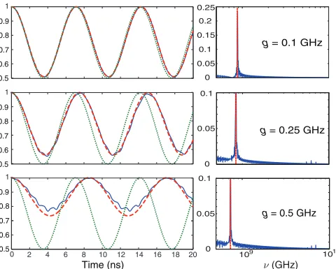
Figure 1 shows a comparison of the dynamics predicted using these expressions and a numerically exact approach. The latter are obtained by imposing a truncation of the oscillator Hilbert space at a point where the dynamics have converged and any higher modes have an extremely low occupation probability. Our zeroth-order approximation proves to be unexpectedly powerful, giving accurate dynamics well into the strong coupling regime (g/ω=0.25) and even beyond this it still captures the dominant oscillatory behavior; see Fig.1. Stronger coupling increases the numerical weight of higher frequency terms in the series, causing a modulation of the dynamics. The approximation starts to break down at (g/ω=0.5). Equations(17)and(18)are obviously unable to capture the higher frequency modulations to the dynamics or any potential long-time phenomena like collapse and revival, but these are unlikely to be resolvable in experiments in any case. Nonetheless, it is worth pointing out that even in this strong coupling case, the base frequency of the qubit dynamics is still adequately captured by our single-term approximation. Our methodology can be used to predict dynamics of nanomechanical resonators connected to either quantum dots or superconducting qubits. The criterion for the single-term approximation to be valid is readily met by current experiments such as those presented in Refs.9and10, and their parameters yield near-perfect agreement between numerical and analytic results. Most experiments operate in a regime where the
0 2 4 6 8 10 12 14 16 18 20
(GHz)
g = 0.1 GHz
g = 0.25 GHz
g = 0.5 GHz
0 0.05
0.1 0.15
0.2 0.25
0 0.05
0.1
109
0 0.05
0.1
1010 1
0.8 0.7 0.6 0.5 0.9 1
0.8 0.7 0.6 0.5 0.9 1
0.8 0.7 0.6 0.5 0.9
Time (ns) ν
FIG. 1. (Color online) Comparison of the single term approximation (red, dashed) and a numerically exact approach (blue, solid) for different coupling strengths. Uncoupled Rabi oscillations are also shown as a reference (green, dotted). Left: the population
ρ00(t) in the time-domain. Right: the same data in the frequency
domain. The full numerical solution was Fourier transformed using Matlab’s FFT algorithm. Other parameters are ω=1 GHz,
==100 MHz, andT =10 mK.
10 0
0.2 0.4 0.6 0.8 1.0
ρ00
(t)
0.8 0.6 0.4 0.2
0 -1 -2
-3 1 2 3
n
Cn
(
τ
=0)
0.25
0.15
0.05
0.1 0.2 0.4 0.6 0.8 1
F(
)
5 0
t (ns) 15
ν
ν
(GHz)
FIG. 2. (Color online) Main panel: comparison of dynamics calculated from truncating Eq.(16)atNMAX= ±10 (red, dashed) and a numerically exact approach (blue, solid). Lower left: Fourier transform of the dynamics. Lower right: the numerical weight of the
nth term in the series expansion of Eq.(16), showing there are still only two dominant frequencies atn=0 andn= −1. Parameters:
ω=0.5 GHz,g=0.1 GHz,=0,=0.5 GHz,T =1 mK.
qubit dynamics are not greatly perturbed by the presence of the oscillator, which has a much lower frequency (≈≈
10 GHz,ω=1 GHz). In Fig.1, we chose≈≈100 MHz, because this better demonstrates the effect of the oscillator on the qubit. These parameters can be achieved experimentally using the same qubit design but with an oscillating voltage applied to the CPB bias gate.11However, we stress the accuracy of our method is not restricted to this regime.
Including extra terms in the series expansion Eq.
(16) makes the time dependence of the qubit dynamics analytically unwieldy, because the rational function form of the series leads to a complex interdependence of the positions of the poles in Eq. (10). However, if the values of the parameters are known, the series can be truncated at (±NMAX) to give an efficient numerical method to obtain
more accurate dynamics, extending the applicability of our approach beyond low temperatures and moderate-to-strong coupling. This is demonstrated in Fig. 2, where the dynamics are clearly dominated by two frequencies – an effect that could obviously never be captured by a single-term approximation. There is a qualitative agreement between the many terms expansion and full numerical solution, particularly at short times. We would not expect a particularly good agreement in this case because the simulations are of the dynamics in the high tunneling regime (=0.5), and the polaron transform makes the master equation perturbative in this parameter. For large tunneling, the traditional numerical approach of oscillator Hilbert space truncation would be more suitable. However, for more moderate tunneling, the rapid convergence of the series is shown in Fig.2;NMAX =5−10
is sufficient to calculateρ00(t) andρ10(t) with an accuracy only
limited by the underlying Born approximation. The asymmetry of the amplitudes of the terms in the series expansion of Eq.
[image:3.608.315.557.69.259.2] [image:3.608.52.292.465.658.2]IV. QUANTUM THERMOMETRY
We now discuss the application of our model system to the measurement of the temperature of an oscillator by observing the coupled qubit. We picture a situation in which the qubit oscillation frequency is the measured quantity. The tunneling, coupling strength, and energy splitting are usually within the control of the experimentalist (or are at least known constants), and this yields the possibility of using the measured to estimate the temperature. A related idea was recently used in the calibration of a seminal resonator experiment10 to verify that the oscillator was in its ground state (a critical part of the work). In that case, the authors used a comparison of numerical results for different occupation numbersNwith the measured population in the excited state of the qubit after a certain interaction time. A theoretical study of the same approach was preformed in Ref.24, where the system was described by the JCM without a tunneling term. They also recently extended their more abstract quantum estimation theory approach to other forms of coupling.25 In contrast, we here propose a practical implementation that uses our simple analytic expressions for the qubit dynamics, which are valid beyond the weak coupling regime, to directly measure the temperature and henceNof the oscillator, simply by observing the effective qubit Rabi frequency.
Figure3demonstrates this idea, showing that by measuring
and fitting it to our Eq.(19), we can obtain submilli-Kelvin
0 10 20 30 40 50 60 70 80 90 100
0 10 20 30 40 50 60 70 80 90 100
Ω
(GHz)
TIn(mK)
TOut
(mK)
0 0.4 0.6
0.5
T (K)5 10
Abs. err. (10
-3)
100 1000 2000
0 1 2
L
FIG. 3. (Color online) Demonstration of qubit thermometry:Tin
is the temperature supplied to the numerical simulation of the system andToutis the temperature that would be predicted by fitting oscillations with frequency Eq.(19)to it. The inner blue line is the data and outer red lines show the effect of a 10 kHz error in the frequency measurement; the gray dashed line serves as a guide to the eye. The lower inset shows the variation of the qubit frequency
with temperature. The upper inset shows the dependence of the absolute error in the prediction against the signal length (see text). Other parameters:ω=1 GHz,g=0.01 GHz,=0,=100 MHz.
precision in the experimentally relevant regime of 20–55 mK. At low temperatures, the single-term frequency plateaus, causing the accuracy to break down. In the higher temperature limit, we also see a deviation from the diagonal, this is to be expected, as we leave the regime where we safely assume the accuracy of the approximation. Naturally accuracy in this region could be improved by retaining higher order terms in Eq. (16), but this would become a more numeric than analytic approach. The upper inset shows the dependence of the accuracy of the prediction on the number of points (at a separation of 1 ns) sampled from the dynamics. The accuracy increases initially as more points improve the fitted value of ; however, after a certain length the accuracy is diminished by long-term envelope effects in the dynamics not captured by the single-term approximation. We note that the corresponding analysis in the frequency domain would not be equally affected by the long-time envelope; however, a large number of points in the FFT is then required in order to obtain the desired accuracy. The lower inset of Fig. 3
shows the direct dependence of on the temperature. The temperature range with steepest gradient and hence greatest frequency dependence on temperature varies with the coupling strength; thus, the device could be specifically designed to have a maximal sensitivity in the temperature range of the most interest.
V. CONCLUSION
In conclusion, we have developed and explored a new approach to the Rabi model, which yields succinct expressions for the qubit dynamics. In contrast to previous theoretical approaches, our expressions are valid in the stronger coupling regime that is rapidly gaining experimental relevance. We have further proposed an application of our model enabling precise temperature measurements of the oscillator mode. This could be used either as part of the calibration of an oscillator experiment or as a tuned, stand-alone device.
ACKNOWLEDGMENTS
We thank Nikesh Dattani, Tom Stace, Gerard Milburn, and Ahsan Nazir for fruitful discussions. This work was supported by the EPSRC, the National Research Foundation and Ministry of Education, Singapore, and the Royal Society.
APPENDIX A: DERIVATION OF THE EQUATIONS OF MOTION
In this Appendix we give the explicit derivation of the equations of motion [Eqs.(6)–(9)] and the bosonic correlation function [Eq.(13)]. We note that parts of these derivations can be found in similar form in the literature (cf. Refs.18–20), but we here give an alternate and full account in consistent notation for the benefit of the reader.
First, we move into the interaction picture:
˜
ρ00(t)=ρ00,ρ˜11(t)=ρ11, (A1)
˜
[image:4.608.52.293.390.628.2]where Dt and Dt† are the time-dependent versions of the displacement operators introduced by the polaron transform:
˜
HI (t)=
2 [(ρ01(t)+ρ10(t)]. (A3) Starting from the Von Neumann equation,
d
dtρ˜(t)= −i[ ˜HI(t),ρ˜(t)], (A4)
we have
˜
ρ(t)=ρ0−i t
0
dt[ ˜HI(t),ρ˜(t)]. (A5)
To study the dynamics we need the time-dependent expec-tation values of the density matrix elements. These are given by
Ot =Tr[ρ(t)O]=Tr[ ˜ρ(t) ˜Ot]. (A6)
Substituting in Eq.(A5),
Ot− O0= −i t
0
dtTr[[ ˜HI(t),ρ˜(t)] ˜Ot]. (A7)
Exploiting the cyclic property of traces,
Ot− O0= −i t
0
dtTr{ρ˜(t)[ ˜Ot,H˜I(t)]}. (A8)
Substituting O for the relevant operator, e.g., ˜ρ00(t), evaluating the commutator, and tracing over the qubit degrees of freedom yields
ρ00(t) − ρ00(0) = −i
2
t
0
dt(ρ10(t) − ρ01(t)),
(A9)
ρ11(t) − ρ11(0) =i
2
t
0
dt(ρ10(t) − ρ01(t)),
(A10)
ρ01(t) − ρ01(0) = −i
2
t
0
dtei(t−t)(ρ00(t)DtD†t
− ρ11(t)Dt†Dt), (A11)
ρ10(t) − ρ10(0) =i
2
t
0
dte−i(t−t)(ρ00(t)DtDt†
− ρ11(t)D†tDt). (A12)
At this point we make the Born approximation (assuming the density matrix of system and bath are factorable)
ρ00(t)Dt(α)Dt(α)t≈ ρ00(t)Dt(α)Dt(α). (A13)
The bosonic correlation function is defined asC(t−t):
C(t−t)= Dt(α)Dt†(α) =TrB[ρBDt(α)Dt†(α)], (A14)
where the subscript B represents the bosonic degrees of freedom. We substitute this into Eq. (A9)and by assuming there is no initial coherence in the system, we obtain Eqs.(6)–(9).
APPENDIX B: BOSONIC CORRELATION FUNCTION The bosonic correlation function Eq.(12)for an oscillator with a single mode in a thermal state is defined as
C(t−t)=TrB[ρBDt(α)Dt†(α)], (B1)
ρB=
exp(−βωa†a) TrB[exp(−βωa†a)
= 1
Zexp(−βωa
†a). (B2)
This can be evaluated in different ways, one of which is presented below. Starting from the time-dependence of the displacement operator in the interaction picture,
Dt(ξ)=eiH0tD(ξ)e−iH0t =eiωa
†at
D(ξ)e−iωa†at, (B3)
or, alternatively, through the time-dependence of creation and annihilation operators,
Dt(ξ)=eξ a
†eiωt−ξ∗ae−iωt
=D(ξ eiωt). (B4)
In order to perform the trace TrBin the number state basis, we need to know the action ofeξ a†a andD(ξ) on a number state|n. The first simply evaluates toeξ n and the latter gives the so-called displaced number state|ξ,n.
The displaced number state can be expanded in the number state basis
|ξ,n = ∞
m=0
Cnm|m, Cnm= m|D(ξ)|n, (B5)
with (see, e.g., Ref.26or27)
Cnm=
n!
m!e
−1 2|ξ|
2
ξm−nLnm−n(|ξ|2), (B6)
whereLmn−n(|ξ|2) is an associated Laguerre polynomial. This is only valid for m > n, but for m < n the displacement operator, or rather its hermitian conjugate, can be made to act onm|instead of on|n.
We use Eq. (B4) for the displacement operator and the propertyD(x)D(y)=e12(xy∗−yx∗)D(x+y) to evaluate Eq.(B2). This leads to a series of the following form:
C(t−t)= 1
Ze
−|α|2[1−e−iω(t−t)]
×∞
n=0
e−βωnLn(2|α|2{1−cos[ω(t−t)]}).
(B7)
By virtue of the property∞n=0Ln(y)zn=(1−z)−1e(yz/(z−1)) and withN =(eβω−1)−1andZ =(1−e−βω)−1, we finally
arrive at the analytical result:
C(t−t)=e−i|α|2sin[ω(t−t)]e−2|α|2{1−cos[ω(t−t)]}(N+1/2). (B8)
Note that this expression agrees with Mahan’s re-sult for a single mode (Ref. 18, Sec. 4.3) C(t)=
e−|α|2[(1−cosωt) coth(βω
*[email protected] †[email protected]
1I. I. Rabi,Phys. Rev.49, 324 (1936).
2B. W. Shore and P. L. Knight,J. Mod. Opt.40, 1195 (1993). 3J. M. Raimond, M. Brune, and S. Haroche,Rev. Mod. Phys.73,
565 (2001).
4R. L. Fulton and M. Gouterman,J. Chem. Phys.35, 1059 (1961). 5E. Jaynes and F. Cummings,Proc. IEEE51, 89 (1963).
6P. Kok and B. W. Lovett,Optical Quantum Information Processing
(Cambridge University Press, Cambridge, 2010).
7T. Niemczyket al.,Nat. Phys.6, 772 (2010).
8P. Forn-D´ıaz, J. Lisenfeld, D. Marcos, J. J. Garc´ıa-Ripoll, E. Solano,
C. J. P. M. Harmans, and J. E. Mooij,Phys. Rev. Lett.105, 237001 (2010).
9M. D. LaHaye, J. Suh, P. M. Echternach, K. C. Schwab, and M. L.
Roukes,Nature (London)459, 960 (2009).
10A. D. O’Connellet al.,Nature (London)464, 697 (2010). 11E. K. Irish, J. Gea-Banacloche, I. Martin, and K. C. Schwab,Phys.
Rev. B72, 195410 (2005).
12E. K. Irish,Phys. Rev. Lett.99, 173601 (2007). 13J. H. Van Vleck,Phys. Rev.33, 467 (1929).
14J. Hausinger and M. Grifoni,Phys. Rev. A82, 062320 (2010). 15J. Hausinger and M. Grifoni,Phys. Rev. A83, 030301 (2011). 16D. Braak,Phys. Rev. Lett.107, 100401 (2011).
17M. Wagner, Unitary Transforms in Solid State Physics, 1st ed.
(North-Holland, Amsterdam, 1986).
18G. D. Mahan,Many Particle Physics: Physics of Solids and Liquids,
3rd ed. (Springer, Berlin, 2000).
19T. Brandes and N. Lambert,Phys. Rev. B67, 125323 (2003). 20T. Brandes,Phys. Rep.408, 315 (2005).
21I. I. Abram and R. Silbey,J. Chem. Phys.63, 2317 (1975). 22E. K. Irish and K. Schwab,Phys. Rev. B68, 155311 (2003). 23D. I. Schuster, A. Wallraff, A. Blais, L. Frunzio, R.-S. Huang,
J. Majer, S. M. Girvin, and R. J. Schoelkopf,Phys. Rev. Lett.94, 123602 (2005).
24M. Brunelli, S. Olivares, and M. G. A. Paris (2011),
arXiv:1103.2875.
25M. Brunelli, S. Olivares, M. Paternostro, and M. G. A. Paris (2012),
arXiv:1205.3465.
26G. C. de Oliveira, A. R. de Almeida, I. P. de Queiros, A. M. Moraes,
and C. M. A. Dantas,Physica A351, 251 (2005).