Saif Ur-Rehman
A Thesis Submitted for the Degree of PhD at the
University of St Andrews
2012
Full metadata for this item is available in Research@StAndrews:FullText
at:
http://research-repository.st-andrews.ac.uk/
Please use this identifier to cite or link to this item: http://hdl.handle.net/10023/3119
This item is protected by original copyright
School of Biology
PhD Thesis
An investigation of human protein interactions using the
comparative method
by
Saif Ur-Rehman
by me, that it is the record of work carried out by me and that it has not been submitted in any previous application for a higher degree.
I was admitted as a research student in [09, 2006] and as a candidate for the degree of PhD in [09, 2007]; the higher study for which this is a record was carried out in the University of St Andrews between [2006] and [2010].
Date …… signature of candidate ………
2. Supervisor’s declaration:
I hereby certify that the candidate has fulfilled the conditions of the Resolution and Regulations appropriate for the degree of PhD in the University of St Andrews and that the candidate is qualified to submit this thesis in
application for that degree.
Date …… signature of supervisor ………
3. Permission for electronic publication: (to be signed by both candidate and supervisor)
In submitting this thesis to the University of St Andrews I understand that I am giving permission for it to be made available for use in accordance with the regulations of the University Library for the time being in force, subject to any copyright vested in the work not being affected thereby. I also understand that the title and the abstract will be published, and that a copy of the work may be made and supplied to any bona fide library or research worker, that my thesis will be electronically accessible for personal or research use unless exempt by award of an embargo as requested below, and that the library has the right to migrate my thesis into new electronic forms as required to ensure continued access to the thesis. I have obtained any third-party copyright permissions that may be required in order to allow such access and migration, or have requested the appropriate embargo below.
The following is an agreed request by candidate and supervisor regarding the electronic publication of this thesis:
Add one of the following options:
(ii) Access to [all or part] of printed copy but embargo of [all or part] of electronic publication of thesis for a period of 2 years (maximum five) on the following ground(s):
publication would preclude future publication;
Date …… signature of candidate …… signature of supervisor ………
Abstract
There is currently a large increase in the speed of production of DNA sequence data as next generation sequencing technologies become more widespread. As such there is a need for rapid computational techniques to functionally annotate data as it is generated. One
computational method for the functional annotation of protein-coding genes is via detection of interaction partners. If the putative partner has a functional annotation then this annotation can be extended to the initial protein via the established principle of “guilt by association”.
This work presents a method for rapid detection of functional interaction partners for proteins through the use of the comparative method. Functional links are sought between proteins through analysis of their patterns of presence and absence amongst a set of 54 eukaryotic organisms. These links can be either direct or indirect protein interactions. These patterns are analysed in the context of a phylogenetic tree.
The method used is a heuristic combination of an established accurate methodology involving comparison of models of evolution the parameters of which are estimated using maximum likelihood, with a novel technique involving the reconstruction of ancestral states using Dollo parsimony and analysis of these reconstructions through the use of logistic regression. The methodology achieves comparable specificity to the use of gene co- expression as a means to predict functional linkage between proteins.
The application of this method permitted a genome-wide analysis of the human genome, which would have otherwise demanded a potentially prohibitive amount of computational resource.
Acknowledgements
I thank the BBSRC for funding my work and making this project possible. I would also like to thank my supervisor, Dr Daniel Barker for his tireless support and good advice. I would like to thank Professor Mike Ritchie, Dr Jeff Graves and Dr Anne Smith for acting as my committee. I would also like to thank Dr Rona Ramsay, Ji-Hiyun Lim, Wim Verleyen, Dr Christoph Echtermeyer and Maria Keays for helpful discussion. I would also like to thank Dr Neil Symington and Dr Herbert Fruchtl for their helpful advice in using cluster-computing resources.
Abstract...2
Acknowledgements ...3
Chapter 1 ...8
1.1 History... 8
1.2 DNA/RNA ... 9
1.2.1 RNA... 10
1.3 Proteins ... 11
1.3.1 Protein secondary structure ... 11
1.3.2 Protein tertiary structure ... 12
1.3.3 Protein quaternary structure ... 12
1.3.4 Protein domains ... 12
1.3.5 Protein motifs ... 12
1.4 Genes ... 13
1.4.1 Structure of a gene... 13
1.4.1.1 Regulatory region of a gene... 14
1.4.2 Transcription... 15
1.4.2.1 Post Transcriptional processing ... 15
1.4.2.1.1 Genetic Code... 15
1.4.2.1.2 Open reading frames ... 16
1.4.2.1.3 Exons/Introns ... 17
1.4.2.2 Post Transcriptional processing (cont)... 18
1.4.2.2.1 RNA splicing... 18
1.4.2.2.2 Capping ... 19
1.4.2.2.3 Polyadenylation... 20
1.4.3 Translation ... 20
1.5 Genomics... 22
1.5.1 Genome annotation... 22
1.5.2 Genome and cDNA assembly ... 23
1.5.3 Gene detection ... 23
1.5.4 Functional annotation of genes... 25
1.5.4.1 Laboratory based techniques... 25
1.5.4.2 Computational methods for functional annotation of genes ... 26
1.5.4.2.1 Alignment based methods ... 26
1.5.4.2.2 Genome context methods... 28
1.5.4.2.2.1 Rosetta stone ... 29
1.5.4.2.2.2 Gene neighbour ... 29
1.5.4.2.2.3 Interolog detection... 29
1.5.4.2.2.4 Phylogenetic profiling ... 29
1.5.4.2.2.5 Comparative methods... 31
1.5.4.2.2.6 Mirror trees... 32
1.5.5 Storage of functional information ... 33
1.5.5.1 GO... 33
1.5.5.1 KEGG ... 33
1.6 Transcriptomics ... 34
1.6.1 Microarrays... 34
1.6.2 Other methods for transcriptome examination ... 34
1.7 Proteomics ... 34
1.7.1 Protein Structure ... 35
1.7.2 Protein interactions ... 35
1.7.2.1 Experimental detection of protein interactions ... 36
1.8 Description of project. ... 37
Chapter 2 ...39
2.1.1 Homology ... 39
2.1.2 Molecular evolution... 40
2.1.2.1 Synonymous and non-synonymous mutations ... 41
2.1.3 Phylogenetic trees... 41
2.1.3.1 Species trees and gene trees... 42
2.1.3.2 Topologies and branch lengths ... 44
2.1.3.3 Bootstrap support values... 46
2.1.3.4 Evolutionary models in tree estimation ... 46
2.1.4 Detection of homology in molecular data ... 47
2.1.5 Multiple sequence alignment... 49
2.1.5.1 Multiple sequence alignment quality filtration... 50
2.1.6 Methods to estimate phylogenetic trees ... 50
2.1.6.1 Distance methods ... 51
2.1.6.2 Discrete character state methods... 53
2.1.6.2.1 Maximum Parsimony ... 54
2.1.6.2.2 Maximum likelihood... 55
2.1.6.2.3 Bayesian Methods ... 56
2.1.6.3 Heuristic search methods ... 57
2.1.8 Model selection in phylogenetic tree estimation ... 60
2.1.10 Phylogenetic analysis using gene presence ... 63
2.2 Methods... 64
2.2.1 Data Selection... 65
2.2.2 Data Acquisition ... 65
2.2.3 Pairwise Alignment ... 69
2.2.4 Orthology Determination... 69
2.2.4.1 Inparanoid ... 69
2.2.4.2 Implementation ... 70
2.2.4.2.1 Design ... 71
2.2.4.3 Application... 72
2.2.5 Phylogenetic profiles ... 72
2.2.5.1 Single copy proteins... 78
2.2.5.2 Proteome content data/tree... 79
2.2.6 Multiple alignment ... 79
2.2.7 Model selection ... 80
2.2.8 Phylogeny reconstruction ... 81
2.2.9 Comparison of protein content tree with super matrix tree ... 82
2.3 Results ... 82
2.4 Discussion ... 93
2.4.1.ML tree ... 93
2.4.2 Proteome content phylogeny ... 94
2.4.3 Conclusion ... 95
Chapter 3 ...96
3.1 Introduction... 96
3.1.1 Hamming distance ... 96
3.1.2 Comparative method ... 97
3.1.2.1 Phylogenetic profile analysis using the comparative method... 97
3.1.3 Co-expression as measured by microarray... 101
3.1.4 Bayesian classifier ... 101
3.2 Methods... 103
3.2.1 Assessing quality ... 103
3.2.2 Training and test data. ... 104
3.2.3 Hamming distance ... 105
3.2.4 Constrained ML... 105
3.2.5 Co-expression of mRNA ... 106
3.3.1 Hamming distance ... 109
3.3.2 Constrained ML... 110
3.3.2.1 Likelihood ratio statistic ... 115
3.3.3 Co-expression of mRNA ... 121
3.3.4 Bayesian classifier ... 124
3.3.5 Method Comparison ... 127
3.4 Discussion ... 128
3.4.1 Low Sensitivities ... 129
Chapter 4 ...130
4.1. Introduction... 130
4.1.1 Ancestral state reconstruction... 132
4.1.1.1 Parsimony ... 132
4.1.1.2 Likelihood ... 133
4.2 Filters ... 134
4.2.1 Hamming distance filter ... 134
4.2.2 Ancestral state reconstruction filter... 134
4.2.2.1 Dollo parsimony... 134
4.2.2.2 Maddison Test for correlated evolution... 136
4.3 Methods... 138
4.3.1 Maddison test for correlated evolution... 141
4.3.1.1 Algorithm... 141
4.3.1.2 Calculation of total number of ways of having x gains and y losses over the tree... 142
4.3.1.3 Calculation of total number of ways of having p gains and q losses in subset k given x gains and y losses over the entire tree ... 143
4.3.1.4 Permutation effects ... 144
4.3.1.5 Evaluation of Maddison test as heuristic for constrained ML ... 148
4.3.2 Modification of test to match Dollo constraints ... 148
4.3.3 Differential parsimony... 150
4.3.4 Dollo-pos/ Dollo-overall ... 150
4.3.5 Test based on logistic regression ... 150
4.3.5.1 Evaluation of logistic regression as a heuristic for constrained ML... 156
4.4 Results ... 157
4.4.1 Maddison test for correlated evolution... 158
4.4.2 Differential parsimony... 160
4.4.3 Dollo-pos ... 161
4.4.4 Dollo-overall... 162
4.4.5 Logistic regression... 162
4.4.6 Hamming distance ... 168
4.5 Discussion ... 168
Chapter 5 ...170
5.1 Introduction... 170
5.1.1 PPI databases ... 170
5.1.1.1 MIPS ... 170
5.1.1.2 BIND... 171
5.1.1.3 MINT ... 171
5.1.1.4 INTACT... 171
5.1.1.5 HPRD... 171
5.1.1.6 DIP ... 171
5.1.1.7 REACTOME... 171
5.1.1.8 STRING ... 172
5.1.1.9 I2D ... 172
5.1.1.10 KEGG ... 172
5.1.1.11 BIOGRID... 172
5.1.1.12 Discussion ... 172
5.1.2 Power law ... 172
5.2.1 Short Branch filtration ... 174
5.2.2 GO term enrichment ... 178
5.2.3 Intersection with other data sources ... 181
5.3 Results ... 182
5.3.1 GO Enrichment... 182
5.3.2 Intersection with known data... 187
5.3.3 Network statistics ... 188
5.4 Discussion ... 189
5.4.1 GO enrichment ... 189
5.4.2 Intersection with known data... 190
5.4.3 Weaknesses... 190
5.4.3.1 Scaling... 191
5.4.4 Conclusions ... 193
Chapter 6 ...194
6.1 Summary of Project... 194
6.1.1 Repeat Analysis ... 199
6.2 Conclusion ... 200
6.3 Future directions... 202
6.3.1 Computational extensions ... 202
6.3.2 Consensus profiles... 202
6.3.3 Correlated evolution of proteins with the presence or absence of phenotypes ... 203
6.3.4 Drug Targets ... 204
References...205
Appendix A Description of divergence of Java implementation of Inparanoid algorithm from Perl implementation. ...223
Appendix B Individual Gene trees for genes in super matrix utilised in construction of Phylogeny...232
Appendix C: Predictions made by constrained ML ...242
Chapter 1
Introduction to computational annotation of protein coding genes
1.1 History
The discovery in the 1940s (Avery et al. 1944) and confirmation in the 1950s (Hershey and Chase 1952) of DNA (deoxyribonucleic acid) as the physical basis for inheritance was a milestone in biological research. It provided for a means to examine the materials and processes underlying phenotypic traits and provided a conceptual link to the other natural sciences. This was rapidly followed by the elucidation of the three dimensional structure of B-DNA (Watson and Crick 1953) which is the form of DNA prevalent in living cells as it is conducive to nucleosome formation (Richmond and Davey 2003). This structure was the now famous double helix. It had been previously established (Beadle and Tatum 1941) that genes exist as discrete regions within the genome whose sequence codes for the sequence of a corresponding chain of amino acids. The genome of an organism is the full set of hereditary material it possesses (Alberts 2010). This is RNA in the case of some viruses and DNA in the case of all other types of cellular organism (Brown 2006). The discovery of the genetic code (Crick et al. 1961) provided information on the mechanism for this production which
operates via initial intermediary transcription into RNA (ribonucleic acid) and then
translation into proteins. (Some genes also code for RNA products such as tRNAs and other non-coding RNAs (Brown 2006)).
In 1996 Saccharomyces cerevisiae was the first eukaryotic genome to be sequenced (Goffeau et al. 1996) via a large collaborative effort. This was followed by the publication of the first multi cellular eukaryotic genome Caenorhabditis elegans in 1998 (C. elegans Sequencing Consortium 1998) and the draft genomes of the vertebrate Homo sapiens soon followed in 2001 (Venter et al. 2001). The application of industrial streamlining and automation to sequencing efforts over the last 20 years as well as more recently with the onset of next generation sequencing technologies there has been almost exponential growth to sequence databases such as NCBI GenBank (Benson et al. 2009). Sequence data without further processing and annotation cannot shed any light on either biological function or evolutionary relationships between organisms. This means that there has been a focus on the development of highly accurate high throughput methods for functional annotation of genes and other functional genomic elements in recent years as the parity between rates of data generation and rates of accurate and verifiable annotation becomes more divergent (Zhu et al. 2007). 1.2 DNA/RNA
DNA itself is made up of a linear backbone of alternating deoxyribose sugar and phosphate residues (Strachan and Read 2004). There is a nitrogenous base attached to the 1’ (one prime) carbon of each individual sugar residue. There are two forms of nitrogenous base present within DNA. One form possesses a single interlocked heterocyclic ring of carbon and
nitrogen atoms. Bases that exist in this conformation are known as pyrimidines (Strachan and Read 2004). The second form of base consists of two interlocked heterocyclic rings of carbon and nitrogen atoms. These bases are known as purines (Strachan and Read 2004). There are two pyrimidines represented within DNA (Strachan and Read 2004). These are cytosine and thymine commonly represented by the abbreviations C and T respectively (Brown 2006). There are also two purines present, adenine and guanine represented as A and G (Brown 2006). The stability of the double helix structure of DNA is maintained through hydrogen bond formation between the pyrimidine-purine pair C and G and hydrogen bond formation between the remaining pyrimidine-purine pair T and A as well as base stacking interactions between adjacent bases (Yakovchuk et al. 2006). Due to structural constraints base pairing can only occur between a pyrimidine and a purine (Brown 2006).
Similarly the other end of the molecule lacks a phosphodiester bond on the 3’ carbon and is known as the 3’ end (Strachan and Read 2004). The sequence of DNA is usually described in the 5’!3’ direction, as this is the direction of DNA replication as well as transcription of RNA using DNA as a template (Strachan and Read 2004). Thus a feature along a DNA molecule is referred to as being upstream of another feature if it is closer to the 5’ end. The length of a DNA molecule is measured in units of individual base pairs (bp).
DNA is a biopolymer and as such can be fully represented by the sequence of its constituent nucleotide bases. Determination of this sequence for a complete organism
effectively represents the DNA blueprints for the construction of that organism, i.e. the amino acid sequences of its constituent proteins and RNA molecules, as well as the regulatory sequences that regulate production of these molecules both spatially and temporally. 1.2.1 RNA
RNA is constructed of similar residues, however the sugar is a ribose as opposed to deoxyribose and the pyrimidine base thymine is replaced with the base uracil commonly represented by the abbreviation U (Strachan and Read 2004). There is a diverse population of RNA molecules produced by the eukaryotic genome. These molecules are involved with a number of processes essential to life, including protein synthesis and regulation of gene expression. A breakdown of general RNA types and their functions is presented in Table 1.1.
Abbreviated Name Full name Primary Function
mRNA Messenger RNA Provides a template for protein
synthesis.
tRNA Transfer RNA Connection of mRNA to relevant
amino acid during protein synthesis.
rRNA Ribosomal RNA Component of protein synthesising
organelles known as ribosomes.
snRNA Small nuclear RNA Component of RNA-protein machine
(involved in post transcriptional modification of mRNA) known as the spliceosome.
snoRNA Small nucleolar RNA Involved in the modification of rRNA
and snRNA
miRNA Micro RNA Involved in the regulation of RNA
stability and translation.
siRNA Short interfering RNA Involved in the targeted degradation of
Table 1.1: General types of RNA molecules with function (Blow 2004).
1.3 Proteins
Protein molecules are polymers comprised of one or more chains of amino acids. A chain of amino acids can also be referred to as a polypeptide chain. Amino acids are molecules that consist of an amino group, a carboxylic group, an R group and a hydrogen atom (Berg et al. 2001). These components are all linked to a central carbon atom known as the ! carbon (Berg et al. 2001). A polypeptide chain is formed when a peptide bond is formed between the amino group of one amino acid and the carboxyl group of another. All polypeptide chains have a free amino group at one end and a free carboxyl group at the other. These are known as the N-terminus and C-terminus respectively (Alberts 2002). The sequence of a polypeptide chain is presented as moving from the N-terminus to the C-terminus (Alberts 2002). A linear polypeptide chain is also considered the primary structure of a protein (Brown 2006).
It is the R group that distinguishes amino acids (Berg et al. 2001). R groups vary in factors such as “size, shape, charge, hydrogen-bonding capacity, hydrophobic
character, and chemical reactivity” (Berg et al. 2001). There are 20 naturally occurring amino acids that are typically utilised by living cells (Alberts 2002).
1.3.1 Protein secondary structure
The interactions of the R, carboxyl, and amine groups of individual amino acids in a polypeptide chain with each other cause polypeptide chains to fold into characteristic
conformations. These conformations are known as the secondary structure of a protein. There are two main types of secondary structure (Brown 2006).
• The ! helix: This is a structure formed by interactions between the carboxyl groups and amine groups of amino acids which are separated by a number intermediate amino acids (Berg et al. 2001).
• The " sheet: This is a structure formed by the interactions between two polypeptide
chains running either parallel or anti parallel to each other (Brown 2006).
• Random coils: In the absence of particular structural imperatives polypeptide chains
1.3.2 Protein tertiary structure
The tertiary structure of a protein is formed by the folding up of the secondary structural constructs formed by the polypeptide chain into a three dimensional configuration (Brown 2006). This configuration is held together a number of chemical forces including hydrogen bonding between individual amino acids and the interactions of hydrophobic amino acids with water (Brown 2006).
1.3.3 Protein quaternary structure
The quaternary structure of a protein is formed by the interactions of multiple polypeptide chains. Quaternary structure is a hallmark of proteins with a complex function (Brown 2006). 1.3.4 Protein domains
A protein domain can be defined as “a substructure produced by any part of
a polypeptide chain that can fold independently into a compact, stable structure” (Alberts 2002). There are a number of recurrent protein domains that are functionally important within the eukaryotic cell. These include:
• Helix turn helix: This is a domain comprised of two ! helices separated by a short strand of amino acids. It is functionally important due to its ability to bind DNA (Brennan and Matthews 1989).
• Transmembrane domain: This is a domain consisting of ! helical structures capable
of passing through the lipid bilayer (cell membrane) that surrounds the cell. These are crucially important in facilitating cell-cell communication and relaying information about the external environment into a cell (Brown 2006).
1.3.5 Protein motifs
Protein motifs are conceptually similar to protein domains in that they are distinct
substructures within a protein molecule (Brown 2006). In contrast with domains they are not able to form outside of the context of the overall protein. Functionally important protein motifs include:
• Leucine zipper: This motif is important in that it facilitates the formation of protein
• Zinc finger: The zinc finger motif is a set of polypeptide chains whose interactions is
stabilised by the presence of zinc ions. It is also present in DNA binding proteins (Brown 2006).
1.4 Genes
As mentioned above the blueprints for the production of given protein and RNA molecules within an organism are contained in subsections of its genome known as genes. A current more specific definition of a gene presented by Pesole (Pesole 2008) defines them as “a discrete genomic region whose transcription is regulated by one or more promoters and distal regulatory elements and which contains the information for the synthesis of functional proteins or non-coding RNAs, related by the sharing of a portion of genetic information at the level of the ultimate products (proteins or RNAs)”.
1.4.1 Structure of a gene
Figure 1.1: General structure of a gene. Adapted from (Maston et al. 2006). 1.4.1.1 Regulatory region of a gene
A typical regulatory region associated with a gene consists of a promoter element and distal regulatory elements (Maston et al. 2006). The promoter element consists of a core promoter and proximal promoter elements and typically spans less than 1 kb (kilobase) pairs (Maston et al. 2006). The core promoter of a gene is the region of DNA at which the proteins primarily responsible for transcription bind and initiate the process of transcription. Well-studied elements of the eukaryotic core promoter include the TATA box and the initiator or Inr sequence (Brown 2006;Strachan and Read 2004). The TATA box generally has a consensus sequence of 5!-TATAWAW-3! where W is A or T (Brown 2006). The INR
sequence has a consensus 5!-YYCARR-3!, where Y is C or T, and R is A or G (Brown 2006). The TATA box and Inr sequence are generally present upstream of a large number of
eukaryotic genes. Generally most of the elements of the core promoter are generally comprised of near identical DNA sequences.
The proximal promoter is generally located a few hundred base pairs upstream of the core promoter element (Maston et al. 2006). This region of DNA typically contains binding sites for other proteins, which contribute to the transcription of the gene but are not the primary mechanism (Maston et al. 2006).
1.4.2 Transcription
A family of enzymes known as RNA polymerases carry out the process of transcription of DNA into RNA in eukaryotic cells (Brown 2006). This process is known as transcription as the fundamental chemical language is not changed (Alberts 2002). There are three RNA polymerases typically encoded by the eukaryotic genome (Strachan and Read 2004). RNA polymerase I and RNA polymerase III tend to transcribe genes which code for functional RNA molecules, while RNA polymerase II is generally utilised for the production of RNA which is further translated into a protein (Alberts 1998). Transcription proceeds via the following general steps (Brown 2006):
• A protein known as TATA binding protein (TBP) binds to the TATA box sequence.
This causes a bend in the DNA molecule.
• This bend provides a recognition signal for other transcription factors to bind to the
DNA creating a structure known as the preinitiation complex (PIC) (Brown 2006). The formation of the PIC also disrupts base pairing thus creating a single stranded DNA template from which the RNA molecule is synthesised.
• RNA polymerase binds to the PIC and them moves along the single strand on DNA
creating a complementary RNA molecule that conforms to base pairing rules. This RNA molecule is known as the primary transcript.
1.4.2.1 Post Transcriptional processing
After the primary transcript has been produced it is subjected to further modifications. In the case of primary transcripts associated with protein coding gene the primary transcript is also known as pre-mRNA (messenger RNA). In order to explain why these modifications occur it is necessary to understand how RNA molecules specify corresponding polypeptide
molecules.
1.4.2.1.1 Genetic Code
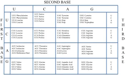
It was established in work by Francis Crick (Crick et al. 1961) that polypeptide chains are specified by RNA molecules via triplets of nucleotides known as codons. As there are only twenty naturally occurring amino acids in eukaryotic proteins, and 43 =64 possible triplets from the 4 nucleotide types, the genetic code is redundant. Three of the codons specify the termination of the polypeptide chain and the remaining 61 specify amino acids.
Table 1.2: The genetic code (Brown 2006).
The process by which these codons are translated into these amino acids will be presented in the next section. This code is widely utilised though there are a number of exceptions where a different code is utilised, e.g. in translation of mitochondrial genes (Knight et al. 2001). 1.4.2.1.2 Open reading frames
Figure 1.2: Starting positions for possible ORFs within a double stranded DNA molecule. 1.4.2.1.3 Exons/Introns
ORFs as discussed above are subsections of the primary transcript or pre-mRNA molecule. ORFs are interrupted within pre-mRNA by sections known as introns (Brown 2006). The sections of the ORF thus separated by the introns are known as exons (Brown 2006). Thus in order to produce a molecule containing the full-uninterrupted ORF it is necessary to excise the introns and splice the exons together as shown in Figure 1.4.
Figure 1.4: Exons post splicing.
Figure 1.5: Exons post splicing in an alternate configuration.
It is not necessary however for all the exons within a given ORF to be utilised (Brown 2006) as shown in Figure 1.5. Different permutations of exons can be created to produce different protein molecules. This process is known as alternative splicing and is responsible for the disparity between the number of genes within a eukaryotic genome and the number of proteins it is capable of producing (Strachan and Read 2004). Alternate splicing is a feature of higher eukaryotes and contributes to overall protein diversity (Black 2003). Estimates of how many human gene products are alternately spliced include 60% (Black 2003) and 74% (Johnson et al. 2003).
1.4.2.2 Post Transcriptional processing (cont)
Having now discussed the necessity of posttranscriptional modification it is now possible to move on to the mechanisms by which splicing is carried out as well as covering other elements of posttranscriptional processing.
1.4.2.2.1 RNA splicing
that introns in pre-mRNA commence with the sequence GU and end with the sequence AG (Strachan and Read 2004). These dinucleotides are not in themselves sufficient to signal a splice junction (Strachan and Read 2004) as splice junctions have been observed to show a greater degree of conservation (Breathnach et al. 1978). In vertebrates the following motifs have been observed at splice junctions (Brown 2006).
• 5! splice site 5!-AG"GUAAGU-3!
• 3! splice site 5!-PyPyPyPyPyPyNCAG"-3!
In these consensus sequences the " symbol indicates the border between an exon and intron or vice versa (Brown 2006). Py indicates that the nucleotide is a pyrimidine and N indicates that any nucleotide could be present at this position (Brown 2006). In addition to the conserved sequences at splice junctions introns also contain a conserved sequence around 40bp away from the end on the intron known as the branch sequence (Strachan and Read 2004). A large RNA-protein complex known as the spliceosome actually carries out the actual process of RNA splicing (Strachan and Read 2004). The spliceosome is one of the largest molecular machines in the human cell containing ~170 distinct proteins (Valadkhan and Jaladat 2010).
The process of RNA splicing typically involves the following sequence (Brown 2006; Strachan and Read 2004):
• Cleavage of the 5’ splice junction detaching the exon from the intron at one end. • The attachment of the cleaved 5’ end to the branch sequence forming a lariat like
structure.
• Removal of the intronic lariat like RNA structure and the ligation of the two
exons. 1.4.2.2.2 Capping
Another step in posttranscriptional modification of protein-coding genes is capping. This process is the first step in posttranscriptional processing of eukaryotic pre-mRNAs (Alberts 2002). This entails the addition of a methylated nucleoside (a nucleoside is a molecule
first 5’ prime end of the transcript (Strachan and Read 2004). This process protects the transcript from rapid degradation via ribonuclease digestion (Strachan and Read 2004). 1.4.2.2.3 Polyadenylation
Post the termination of transcription the primary transcript is also modified via the addition of about 200 adenosine nucleotides to the 3’ end of the transcript (Alberts 2002). This structure is known as a poly-A tail. The process is thought to facilitate the transport of the mature mRNA molecule into the cytoplasm (Strachan and Read 2004).
1.4.3 Translation
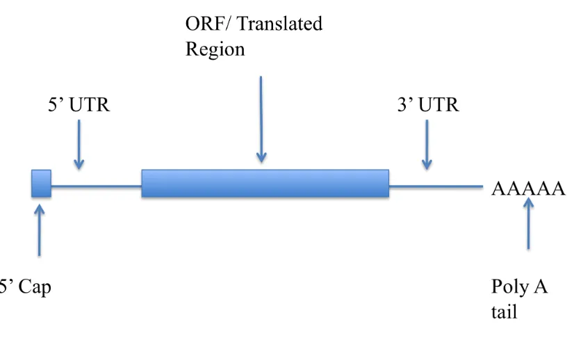
[image:22.595.80.493.445.693.2]After a transcript associated with a protein-coding gene has been transcribed and processed, it then migrates to the cytoplasm, where a process known as translation occurs. This process entails the production a polypeptide chain that is specified by the transcript via the genetic code. The mature mRNA molecule is not synonymous with an ORF (Strachan and Read 2004). Generally an ORF is a subsection within the mature transcript. The ORF is flanked by sequences known as the 5’ UTR and 3’UTR (UTR=untranslated regions) (Brown 2006) as illustrated in Figure 1.6.
Figure 1.6: Schematic of mature mRNA.
The larger subunit is known as the 60S subunit and consists of three different types of
ribosomal RNA (rRNA) molecule and up to 50 ribosomal proteins (Strachan and Read 2004). The smaller subunit is known as the 40S subunit and contains a single rRNA molecule and over 30 ribosomal proteins (Strachan and Read 2004). The two subunits of the ribosome exist as separate entities and attach for the process of translation.
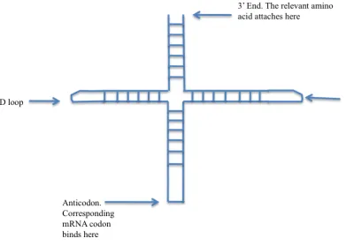
The other molecule that provides the physical basis for the implementation of the genetic code is transfer RNA (tRNA). tRNA has a secondary structure consisting of four double helical structures as illustrated in Figure 1.7. tRNA attaches to an amino acid at its 3’ end. The anticodon arm of the tRNA molecule has a triplet sequence, which is
[image:23.595.80.471.330.609.2]complementary to the codon of the amino acid to which it is bound. Thus tRNA attaches codons to their corresponding amino acids.
Figure 1.7: Structure of a tRNA molecule. Adapted from (Alberts 2008).
The process of translation typically proceeds via the following steps (Strachan and Read 2004):
• The mRNA molecule is then pulled through the ribosome.
• When a start codon is encountered a tRNA molecule with an anticodon arm
complementary to the start codon enters the ribosome. This tRNA molecule will have the relevant amino acid pre-bound to it.
• The next tRNA corresponding to next codon will then enter the ribosome. • The amino acid attached to the first tRNA will detach from the tRNA and attach
to the amino acid attached to the 3’ end of the second tRNA.
• This process is iterated constructing a polypeptide chain or protein molecule. • When a stop codon is encountered an enzyme known as a release factor causes the
ribosome to disassociate and release the protein molecule.
• In order to prevent premature folding of proteins during translation the emerging
polypeptide chain is stabilised by proteins known as chaperones (Alberts 2008). 1.5 Genomics
The term genome can de defined as the “entire genetic complement of a living organism” (Brown 2006). The field of study around ascertaining information about the genome of a living organism is thus known as genomics. The primary step of any full genomic study is the determination of the DNA sequence of the genome of the organism in question. Once this has been determined the next step is annotating the sequence.
1.5.1 Genome annotation
The full genome of an organism is generally a mosaic of functional and non-functional elements. The percentage of an organism’s genome that is functional is variable. In the case of the human genome it has been calculated that potentially between 2.56% and 3.25% is functional (Lunter et al. 2006).
Functional elements in a genome include:
• Genes.
• DNA binding sites.
• CpG Islands: These are stretches of the dinucleotide repeat CG. These areas of DNA
Genome annotation can be described as the systematic location of these functional elements within a genome sequence (structural annotation) and the ascertainment of that function (functional annotation). The location of functional elements is based on the principle of sequence specifying function. Thus the sequence of a functional element will vary in some detectable way from the remainder of the background sequence.
1.5.2 Genome and cDNA assembly
The initial challenge post the generation of sequencing data is the fact that the output of DNA sequencing is generally reads of short stretches of DNA. These reads range in length from > 700 bp long for Sanger sequencing (Hert et al. 2008) and ~200bp for pyro sequencing (Sundquist et al. 2007) and down to ~50bp for ligation based sequencing methods (McKernan et al. 2009).
These short reads have to be assembled into a full sequence for the whole genome. This process is known as contig assembly. Contig assembly is carried out through scanning a set of short reads for overlaps. The discovery of an overlap indicates that two fragments are contiguous and should be connected. This process is necessary both at the level of the full genome as well at the level of the individual gene (Wang et al. 2005a).
1.5.3 Gene detection
Given a fully sequenced and assembled genome lacking annotation there are a number of computational techniques available to delineate coding sequence. These can be divided into two main subtypes: extrinsic and intrinsic (Borodovsky et al. 1994). Extrinsic methods utilise comparisons of sequence data to an external reference point while intrinsic methods evaluate sequences based on properties that are internal to the sequence (Borodovsky et al. 1994).
Construction of a cDNA library is one of the standard methods of extrinsic gene detection. cDNA stands for complementary DNA and is created through application of an enzyme known as reverse transcriptase to mature mRNA. Reverse transcriptase as the name implies reverses the process of transcription and creates a DNA strand complementary to the single stranded mRNA. Further steps are then taken in order to create a double stranded DNA molecule (Strachan and Read 2004).
polymerase chain reaction (PCR) (Mount 2004) and then sequenced. The library of sequences thus generated corresponds to the sequence of protein coding genes within the genome minus the introns. These sequences are then systematically mapped onto the genomic sequence using local alignment algorithms. This technique is known as cis-alignment. There are a number of local sequence programs that can be used to carry out these alignments. Exonerate is one such program. It utilises a bounded dynamic programming approach (Slater and Birney 2005) to generate local alignments. Dynamic programming is discussed in more detail later in this chapter. Another program, which can be utilised, is Spidey (hosted by the NCBI). This program employs the Blast heuristic algorithm (Altschul et al. 1990) to generate its
alignments. SIM4 is another program that utilises an algorithm based on Blast but tailored to the specific problem of mapping cDNA to genomic DNA by factoring in introns and
potential sequencing errors (Florea et al. 1998).
The Ensembl automatic genome annotation system (Curwen et al. 2004;Potter et al. 2004) uses the algorithm GeneWise (Birney et al. 2004) to map cDNA to full genomic data and the algorithm GenomeWise (Birney et al. 2004) to create a final putative structure for the gene in question post the initial alignment. cis alignment can be considered to be one of the most reliable methods for protein coding gene detection/prediction (Brent 2008).
In cases where cDNA libraries are not available or incomplete for the organism under consideration it is also possible to use cDNA sequences of homologous genes from either the same species or a different species in order to detect coding sequence. This technique is also referred to as trans-alignment and is central to various gene prediction tools (Brent 2008). The GeneWise (Birney et al. 2004), algorithm is also used in this context by the Ensembl pipeline (Potter et al. 2004). Extrinsic methods for genome annotation are far more cost and labour intensive as opposed to the strictly in-silico intrinsic approach.
Intrinsic approaches to gene detection are predominantly computational and as such require an explicit definition/description in order to delineate between coding and non-coding sequence (Picardi and Pesole 2010). Picardi (Picardi and Pesole 2010) gives a good working definition of a gene for detection purposes, which defines a gene as a transcribed region of DNA whose expression is regulated by cis acting elements such as upstream promoters. Examples of tasks undertaken as a part of intrinsic gene detection include:
• ORF (Open Reading Frame) detection: Detection of a potential ORF in genomic
detection drastically reduces the search space for potential genes in the case of prokaryotes.
• Promoter regions detection: Genes are typically associated with one to several
promoter regions. In prokaryotes these include the upstream Pribnow box with the consensus sequence TATAAT. This sequence is homologous to the eukaryotic TATA box (Berg et al. 2007). Detection of these motifs within a sequence upstream of an ORF strengthens the case for a potential gene.
• Internal splice junction detection: As the sequence of exon intron borders is broadly
conserved discovery of splice junctions can also contribute to the case for a prospective gene.
These features can be can be detected within a stretch of sequence using various techniques to model sequence motifs ranging from simple regular expressions to hidden Markov models and position weight matrices (Picardi and Pesole 2010). Examples of specific applications of the intrinsic approach to gene prediction include SNAP (Korf 2004) and Genscan (Burge and Karlin 1997) both of which utilise Markov models in order to detect delineating features of genes. The primary weaknesses of the intrinsic approach lie in the fact that that it requires a representative sample of protein coding genes specifically from the organism under consideration in order to operate (Aubourg and Rouze 2001).
1.5.4 Functional annotation of genes
After a putative gene has been identified the next stage is determination of the exact
biological role of the product coded for. This process can be carried out computationally or by entirely laboratory based techniques.
1.5.4.1 Laboratory based techniques
Laboratory based techniques for determination of biological function involve alteration of the gene in question either in the organism of study (in the case of prokaryotes, unicellular eukaryotes as well as higher eukaryotes which are deemed suitable) or in the case of organisms where modification would be impractical or unethical such as Homo sapiens alteration of the homologous gene in a model organism. The main model organism of choice for study of mammalian gene function is Mus musculus (Kim et al. 2010). The main
• Knockouts: This entails the removal of the gene in order to observe the effects of its
absence. This technique is only effective if the gene in question is not essential to organism survival and has a visible/measurable effect on phenotype (Moore 1999).
• Alteration in expression: In cases where the gene in question is essential to the
survival of the organism, alterations can be made to the cis-regulatory regions of the gene in question in order to affect levels of expression (Capecchi 2005).
• In order to physically pinpoint specific tissues (in the case of multi-cellular
organisms) or areas within a cell that a protein is active it is possible to place a reporter gene such as GFP (green fluorescent protein) upstream of the promoter region of the gene of interest (Chalfie et al. 1994).
• Detection of genetic interactions: The interaction of two non-essential genes (and
hence their associated proteins) can be detected if the mutation of both genes leads to lethality (von Mering et al. 2002). This method has been applied to a large-scale study in Saccharomyces cerevisiae in order to characterise its set of genetic interactions (Ooi et al. 2006). The detection of an interaction partner of known function can aid in the determination of the function of an unknown gene.
1.5.4.2 Computational methods for functional annotation of genes
Computational methods to determine gene function have only become applicable relatively recently as most computational methods depend on comparison of novel sequence data with sequence of known function. Computational methods of functional annotation of genes can be split into a number of broad categories (Pellegrini 2001).
• Alignment based methods. • Genome Context methods.
1.5.4.2.1 Alignment based methods
derived functional annotation can be applied to all members. Alignment methods can be applied at either the gene or the protein level.
There are three primary ways of carrying out pairwise sequence alignments.
• Dot matrix analysis: This method entails arranging one sequence horizontally and the
other sequence vertically perpendicular, starting from the left end of the horizontal sequence. Matches between the two sequences are then marked with a dot. Areas of similarity can then be viewed as diagonal lines between the two sequences (Mount 2004).
• Dynamic programming: Dynamic programming is a programming paradigm which
entails the reduction of a large problem to a series of sub-problems whose solutions are constructed incrementally and summed to provide the overall solution (Russell et al. 2003). In terms of sequence alignment it entails the construction of a matrix similar to the dot matrix and calculating a path through it, where the next step in the path is determined only by the state of the current cell and its neighbouring cells. Two popular dynamic programming algorithms utilised in pairwise alignment of sequences are the Needleman-Wunsch algorithm (Needleman and Wunsch 1970) which returns an optimal global alignment of two sequences and the previously mentioned Smith-Waterman algorithm (Smith and Waterman 1981) which provides an optimised local alignment. Both of these algorithms are proven to return the optimal alignment between two sequences (Mount 2004).
• Heuristic Algorithms: Both the dynamic programming algorithms mentioned above
are O(n2) in terms of both memory utilisation as well as time taken to run (Mount 2004). As such heuristic algorithms such as Blast (Altschul et al. 1990) and Fasta (Pearson and Lipman 1988) were developed as usable alternatives. The Fasta algorithm constructs a sequence alignment by searching for matching sequence patterns called k-tuples. These patterns are k consecutive matches between the two sequences. These matches are then extended to provide the alignment (Krane and Raymer 2003). Blast constructs an alignment in a similar manner by locating short matches and then building an alignment around it. The difference between Blast and Fasta is that while Fasta examines all possible k-tuples the Blast algorithm is
judged through use of the BLOSUM62 substitution matrix (Mount 2004). Given the rapid expansion of most of the large sequence databases it is typical to use heuristic algorithms as a search tool.
• Profile Hidden Markov models have been used by Eddy (Eddy 1998) to create a
scoring system, which allows detection of remotely homologous sequences. Hidden Markov models score the probability of a discrete chain of events based on model parameters whose values are unknown (Durbin 1998).
Alignment methods can also be applied to the three dimensional structures of protein molecules as well as sequence (Hasegawa and Holm 2009). This method is potentially useful in cases where sequence divergence reaches a point where two proteins can no longer be identified as homologous. However as the rate of structure generation lags behind sequence generation by a considerable degree this method can only be applied in a small subset of cases.
Detection of a significant alignment with a gene of known function can be used to attach the same function to a gene of known function. Martin (Martin et al. 2004) used GO terms (Ashburner et al. 2000) in conjunction with Blast (Altschul et al. 1990) to achieve this with some success. There is however a danger with alignment based methods of a “Chinese whispers” effect where if for example a gene p with known function a displayed 90 % identity using some form of pairwise alignment algorithm with gene q of unknown function. Assigning function a to gene q would seem to be intuitively legitimate. However if gene q was assigned function a and the process was iterated a number of times a situation could arise where a gene x would be assigned function a with little or no sequence similarity to the original protein p. Examples of incorrect annotation by automated methods of homology detection occur in the case of genes where translations of the antisense strand of the coding region are entered into databases such as GenBank (Linial 2003).
1.5.4.2.2 Genome context methods
Thus through demonstration of functional association or interaction between one gene/protein of known function with one of unknown function, the latter entity may be annotated with the function of the former.
1.5.4.2.2.1 Rosetta stone
The Rosetta stone method or detection of domain fusion was recognised through work by Marcotte (Marcotte et al. 1999) and Enright (Enright et al. 1999) which showed that sets of separate proteins in one organism which exist in a unified (fused) homologous form in another organism are likely to be interaction partners. As fusion events are comparatively rare and generally affect genes that are tightly functionally coupled this method is effective at detection of interaction partners (Kensche et al. 2008). However the rareness of these events lowers the overall coverage of this method.
1.5.4.2.2.2 Gene neighbour
Examination of the genomes of nine bacterial and archaeal genomes by Dandekar (Dandekar et al. 1998) showed that the proteins encoded by genes which showed conserved physical order along a chromosome tended to interact physically.
1.5.4.2.2.3 Interolog detection
A term introduced by Walhout (Walhout et al. 2000) an interolog is a pair of proteins that interact in a given organism. If both proteins involved in the interaction are conserved in another organism a similar interaction can be inferred in the second organism. This method has shown comparable accuracy with large-scale experimental data (Yu et al. 2004b).
1.5.4.2.2.4 Phylogenetic profiling
mutation in upstream cis-regulatory sequences thus removing the potential for transcription (Brown 2006). Pseudogenes can also be formed through retrotransposition of mature mRNA (Graur et al. 1989).
Thus through examination of multiple genomes for correlations in the presence and absence of proteins potential functional linkages can be detected. A phylogenetic profile is typically a binary string representing the presence or absence of a homolog of a given
gene/protein. Predictions are made through examination of levels of similarity between these strings. These suggestions are suggestive in their nature rather than specific as it is unclear what the nature of a functional linkage between two proteins with similar profiles might be. The relationship could be a direct physical interaction such as subunits involved in
heterodimerisation or more indirect such as the link between a transcription factor and the product of its associate gene.
The first use of phylogenetic profiles to predict functional linkages used Hamming distance as a metric in order to cluster similar profiles (Pellegrini et al. 1999). The Hamming distance of two strings can be defined as the number of points at which they differ (Hamming 1950). There have been various extensions and reinterpretations of the method since then (Ranea et al. 2007). Some of these involved examination of profiles using higher logical operations to carry out more complex comparisons of profiles (Bowers et al. 2004; Antonov and Mewes 2008). The method was also applied to protein domains rather then whole
sequences (Pagel et al. 2004b). Work by Ranea utilised domain information from the Gene3D database to create phylogenetic profiles of the presence and absence of structural domains within genomes (Ranea et al. 2007). This method thus bypasses the problem of identification of genes that are functionally homologous by focussing on the presence and absence of predefined domains within proteins. Chen and Vitkup used examination of correlation coefficients to measure similarity in phylogenetic profiles (Chen and Vitkup 2006). They observed that the method was successful in identifying genes that were members of the same metabolic pathways (Chen and Vitkup 2006).
As a tool phylogenetic profiling could be used to detect errors in genome annotation through the detection and displays of gene absences, which are not plausible in closely related species. A similar approach has in fact been used by Pinney to detect and annotate enzyme-coding genes in the protist E. tenella (Pinney et al. 2005).
Other extensions to the method involved the utilisation of the phylogenetic
This method made use of an explicit phylogeny and ancestral reconstruction over the phylogeny based on a continuous-time Markov model. The likelihood of a model of dependent or contingent evolution was compared with the likelihood of a model of independent evolution over the phylogeny. This method was then further extended by investigating the effects of constraining the rate at which genes could be acquired over the phylogeny (Barker et al. 2007).
Other methods of incorporating phylogenetic information included the work by Vert (Vert 2002), which utilised support vector machines, as well as the work by Cokus (Cokus et al. 2007), which utilised phylogeny as a heuristic by ordering profiles by the phylogenetic closeness of the organisms involved.
1.5.4.2.2.5 Comparative methods
Comparing phylogenetic profiles over a phylogenetic tree can be considered to be an application of the comparative method to traits at the molecular level. The comparative method is a well-established method in biology (Harvey and Pagel 1991). The fundamental idea of underpinning the comparative method is how the state of one factor (which can be a trait or environmental condition) influences the state of another over the context of a topology of a phylogenetic tree (Maddison 1990). Testing for correlations without considering the phylogeny will detect correlations in gene content based on phylogenetic relationships rather than functional linkage. For example the set of all genes that are intrinsic to the class Mammalia will share similar phylogenetic profiles. This does not however suggest that they are all functionally linked.
There are a number of tests that have been developed in order to test the correlations in the states of traits over a phylogeny. Ridley (Ridley 1983) developed one of the earliest of these tests. This test involved the construction of a 2x2 contingency table where the state of each trait was considered as a categorical variable defined at each node in the tree. The method assumed that the construction of an accurate phylogeny and accurate reconstruction of ancestral context for each node within the phylogeny. Ridley’s method did not however differentiate between dependant and independent variables in measuring the significance of a given set of changes (Maddison 1990). The method did not take into account the sequence of changes in the states of traits (i.e. was a change in state A followed by a change in state B or vice versa). This makes the results of the method difficult to interpret (Maddison 1990).
over a tree as a Brownian process. Another test for detection of correlations in traits and/or external environmental conditions was devised by Grafen. This test was a phylogenetically corrected regression, which did not rely on any form of ancestral reconstruction (Grafen 1989).
Maddison developed a similar test to Ridleys in 1990 (Maddison 1990). It however did distinguish between dependant and independent variable by defining areas of a phylogeny to be in state A or state B depending on the state of one of the traits under consideration. The test then measured how many of the changes in the other trait occurred in the area of the tree that was in state A compared to how many changes were possible over the whole tree.
One of the issues with the tests described above was the fact that none of them
integrated information on branch lengths of the phylogeny. This meant that the probability of a change in the state of a given trait was equally likely over a branch of a phylogenetic tree regardless of its length. However clearly a change on a short branch is less likely than a longer branch. Work by Pagel took this into account by integrating branch lengths into a test for correlated evolution (Pagel 1994). The parameters defined by this work were utilised by Barker and Pagel in their approach to phylogenetic profile analysis (Barker and Pagel 2005).
1.5.4.2.2.6 Mirror trees
Another method of detection potential protein interactions is known as mirror trees. This method involves the detection of protein interactions through the construction and comparison of phylogenetic trees of proteins with a single genome (Pazos and Valencia 2001). The rationale behind this method is similar to that of phylogenetic profiling. However correlation is sought not in the presence and absence of homologous genes but in the pattern of sequence evolution of interacting proteins. Trees are examined by examining distance matrices of homologous sequences for correlations. These matrices are the inputs used in the formation of the trees in question. The phylogenetic tree of any given protein in a genome will however carry signal from the speciation events, which shaped the genome of the
the phylogenetic trees of functionally linked genes is more likely to be due to chance or as mentioned above due to background similarity.
1.5.5 Storage of functional information
With the exponential increase in sequence data that has been generated through the 2000s there have been a number of attempts with which to organise and contextualise function information surrounding genomic entities.
1.5.5.1 GO
A notable attempt to do this has been the establishment of a controlled vocabulary with which to describe the functional role of a gene as well as its physical location within the cell. The vocabulary is known as the Gene Ontology (GO) (Ashburner et al. 2000). GO associates a set of terms with gene products. These terms are known as GO terms and fall into three general domains. These are
• Cellular component: This is the physical location within the cell where the gene
product is generally to be found.
• Biological process: This is the biological pathway or process that the gene product has
been localised in.
• Molecular function: This is a lower level to the biological process domain and
includes the specific molecular capabilities of the molecule in question. An example of molecular function could be the ability to bind a particular metal.
Terms are organised as a network starting from the root terms defined above. As the network is traversed starting from a root term, terms become more specific, i.e. if term B is directly below term A in the ontology then term B is a subclass of term A.
1.5.5.1 KEGG
1.6 Transcriptomics
The transcriptome of a cell can be considered to be the sum total of its genome that is transcribed into RNA. Studying the transcriptome can also yield insights into the functionality of gene products.
1.6.1 Microarrays
At the transcriptomic level the putative function of a gene can be at least partially determined through establishing the association of the expression of a particular gene with a particular external condition or treatment. This can be achieved through the use of glass slides known as microarrays (Mount 2004). These slides have oligonucleotides, which are subsections of a set of genes attached to them. Cells of the organism under study are subjected to variable experimental conditions. mRNA is then extracted from these cells, converted to cDNA and fused with a unique florescent dye. By examining the relative degrees of florescence for the colours associated with the two versions of the cDNA of the gene of interest it is possible to measure levels of gene expression in response to a given experimental condition. A variant of this involves using full cDNA molecules as the contents of the chip.
1.6.2 Other methods for transcriptome examination
Expression levels for a given environmental condition can also be measured through direct sequencing and counting through use of the SAGE (Serial analysis of gene expression). In this method mRNA is extracted from the cells of interest. A small section is excised from each mRNA molecule. A tag is then connected to each separate subsection. These
subsections are then amplified and the tags counted thus providing a measure of gene
expression levels (Velculescu et al. 1997). Another protocol for sequencing mRNA to detect gene expression levels has also been developed. This protocol is known as RNA-Seq and is made feasible through the utilisation of the high throughput nature of next generation sequencing (Wang et al. 2009b).
1.7 Proteomics
Proteomics in a similar way to genomics and transcriptomics is the study of the full protein complement produced by a cell. The proteomic level is the point where the connection between macromolecules and measurable phenotypes is first bridged. Proteins can be
1.7.1 Protein Structure
There are two main methods utilised to determine the three dimensional structure of a protein molecule (Brown 2006). These are:
• X-Ray crystallography: This procedure involves the production of a crystal from the
protein of interest. X-rays are then fired through this crystal to acquire a backscatter diffraction pattern. This diffraction pattern can then be used to reconstruct the
structure of the protein. X-ray crystallography is limited by the fact that it requires the protein to be able to crystallise (Brown 2006).
• NMR spectroscopy: NMR or nuclear magnetic resonance is electro-magnetic
radiation produced by the absorption and re-emition of electro-magnetic radiation by the nuclei of atoms. By bombarding a protein with electro-magnetic radiation, these patterns of resonance can be used to work out the structure of the protein (Brown 2006).
1.7.2 Protein interactions
In terms of protein interactions there are two primary modes of protein interaction. The first is a direct physical interaction. Direct physical interactions between distinct proteins can occur in two contexts (Orengo et al. 2003). These are:
• Formation of a stable complex: A protein complex is a stable structure formed by two
or more proteins to carry out a specific function. In order to maintain the structural integrity of a complex proteins within the complex have to maintain relatively long term direct physical interactions. The subunits of the ribosome are an example of a stable protein complex as well as the histone octamer and RNA polymerases (Orengo et al. 2003). Not all interactions within a protein complex are direct as members of a complex with more then two interacting partners do not necessarily have to be physically connected to every other protein within that complex.
• Transient interaction: These are functional interactions where proteins physically
The other form of interaction between proteins is indirect interactions. Examples of these could be two proteins that have a role in a given metabolic pathway but whose production is temporally and spatially separated. Examples of indirect interactions include the interaction between SHC-transforming protein and mitogen-activated protein kinase 1 over several steps of the insulin-signalling pathway (Sasaoka and Kobayashi 2000).
The full collection of all protein interactions within a cell has been labelled the interactome. 1.7.2.1 Experimental detection of protein interactions
Protein interactions can be detected using a variety of techniques. The main techniques include:
• Yeast two-hybrid: In order to detect protein interactions one widely used (Marcotte et
al. 1999) method is the yeast two-hybrid technique. This technique exploits the S. cerevisiae GAL4 transcription factor. This transcription factor has two domains that require physical proximity in order to operate. One of these domains binds DNA and the other domain is an activator for the transcription factor. A protein interaction can be detected by fusing two genes of interest to both of these domains respectively on separate plasmids and insertion of these plasmids into a yeast cell with a reporter gene upstream of the GAL4 transcription factor-binding site. Reporter gene transcription is only possible if the protein products of the two genes of interest were able to maintain a physical interaction (Griffiths 2002). The primary drawbacks to this method are the facts that all interactions must take place in the nucleus removing a large number of proteins from their native cell compartment and that only binary protein interactions can be tested for (von Mering et al. 2002). The yeast two-hybrid method does have a high rate of false positives. One reason for this is that pairs of proteins that stick together are not necessarily ever expressed at the same time or in the same tissue (Vidalain et al. 2004). Also some proteins such as heat shock proteins are inherently promiscuous in their binding affinities (Vidalain et al. 2004).
• Proteome chips: In a manner similar to the use of microarrays described above for the
• Mass spectrometry of purified complexes: In order to detect interactions that are not
binary, complexes of proteins can be isolated using techniques such as tandem affinity purification. This technique entails the tagging of a protein of interest with a tag that allows the purification of the main protein and any complex partners that it might have. These complexes can be characterised through the use of mass spectrometry (von Mering et al. 2002).
1.8 Description of project.
This work details the development and application of a novel heuristic which combines application of the Barker and Pagel approach to phylogenetic profiling (Barker et al. 2007; Barker and Pagel 2005) in conjunction with a novel data filter. The Barker and Pagel approach to phylogenetic profiling will subsequently be referred to as constrained ML (maximum likelihood). It was observed over the course of this project that this method could be useful in elucidating novel protein interactions. Novel protein interactions will allow further elucidation and annotation of protein function through the principle of guilt by association as articulated above. The proteome of Homo sapiens is still filled with known unknowns in terms of protein-protein interactions. The HPRD (Prasad et al. 2009) currently contains 38,788 binary protein interactions and data on 998 protein complexes. Current estimates of the interactome size such as work by Stumpf (Stumpf et al. 2008), which
estimates the size of the interactome as 650,000, intimate that the majority of protein-protein interactions have not yet been elucidated. The potential of phylogenetic profiling to detect novel interactions has been demonstrated in work by Ramazzina (Ramazzina et al. 2006) where two novel genes involved in the degradation of uric acid were detected. The phylogenetic profiling method has also been successful in identifying enzymes of the MEP/DOXP pathway (Cunningham et al. 2000).
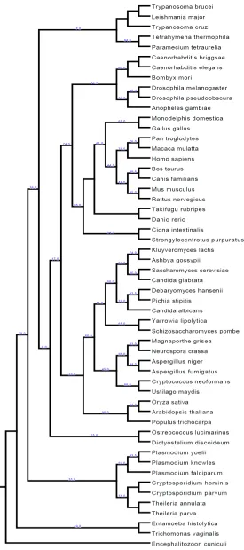
Chapter 2 details the construction of a eukaryotic phylogeny over 54 taxa as well as the phylogenetic profiles of known proteins within the human genome relative to the other 53 species which was one of the essential precursor steps to this study.
Chapter 3 contains the results of the application of the method in context and
al. 2009; Scott and Barton 2007). This system makes novel predictions through the combination of different informative features.
Chapter 4 describes the construction of the data filter, which is based on Dollo parsimony. The filter reduces the size of the overall search space facilitating the use of the method for whole genome comparisons. This is achieved through the elimination of pairs of proteins, whose function cannot be detected via examination of patterns of presence and absence.
Chapter 5 presents a network of predictions generated as a putative human interactome of proteins, which are susceptible to this line of enquiry. This network is analysed for consistency with known data. A set of novel predictions is presented.
Chapter 2
Reconstruction of eukaryotic phylogeny as precursor to comparative
analysis
2.1 Introduction
Examination of the evolutionary histories of organisms is a fundamental step for any form of study of biological function as adaptation can only be examined within an historical context (Harvey and Pagel 1991). As a phylogeny is by definition an evolutionary history of species (Harrison and Langdale 2006) it is a necessary step within the process of a comparative study. In terms of examination of changes in gene content within a probabilistic framework it provides the necessary topology over which such changes occur. This is a fundamental parameter in any such model.
2.1.1 Homology
The fundamental object of any phylogenetic study, whether molecular or morphological, is the comparison of homologous structures within the organisms under consideration. When genomic data is under consideration homologous structures within organisms correspond to those genomic elements, which were present in the last common ancestor of the set of organisms under consideration. These elements can provide a measure of divergence (Fitch 1970). These elements if functional (which is implied by conservation) can either maintain their ancestral function or if sufficiently diverged have a new (or no) function. In discussions of elements of genomes (genes) there are a number of subclasses of homologous
relationships. These are:
• Orthology: Genetic elements are orthologous if they are the direct product of
divergence from a common ancestral species (speciation) (Fitch 1970).
• Paralogy: Genetic elements are paralogous if they are the product of a duplication
event within a given species. Mechanisms of duplication include retrotransposition (insertion of reverse transcribed RNA back into a genome) and unequal crossover leading to tandem duplication of a portion of a chromosome (Hurles 2004). It is thought that these duplication events are a major force in creating and broadening genetic repertoires (Zhang 2003).
• Xenology: Genetic elements are xenologous if they are the product of a direct