warwick.ac.uk/lib-publications
Original citation:
Englert, Matthias, Röglin, Heiko and Vocking, Berthold. (2016) Smoothed analysis of the
2-Opt algorithm for the general TSP. ACM Transactions on Algorithms , 13 (1). 10.
Permanent WRAP URL:
http://wrap.warwick.ac.uk/81525
Copyright and reuse:
The Warwick Research Archive Portal (WRAP) makes this work by researchers of the
University of Warwick available open access under the following conditions. Copyright ©
and all moral rights to the version of the paper presented here belong to the individual
author(s) and/or other copyright owners. To the extent reasonable and practicable the
material made available in WRAP has been checked for eligibility before being made
available.
Copies of full items can be used for personal research or study, educational, or not-for profit
purposes without prior permission or charge. Provided that the authors, title and full
bibliographic details are credited, a hyperlink and/or URL is given for the original metadata
page and the content is not changed in any way.
Publisher’s statement:
"© ACM, 2016. This is the author's version of the work. It is posted here by permission of
ACM for your personal use. Not for redistribution. The definitive version was published in
ACM Transactions on Algorithms, 2016 13,1,10
http://doi.acm.org/10.1145/2972953
"
A note on versions:
The version presented here may differ from the published version or, version of record, if
you wish to cite this item you are advised to consult the publisher’s version. Please see the
‘permanent WRAP url’ above for details on accessing the published version and note that
access may require a subscription.
Smoothed Analysis of the 2-Opt Algorithm for the General TSP
MATTHIAS ENGLERT, University of Warwick
HEIKO R ¨OGLIN, University of Bonn
BERTHOLD V ¨OCKING, RWTH Aachen University
2-Opt is a simple local search heuristic for the traveling salesperson problem, which performs very well in experiments both with respect to running time and solution quality. In contrast to this, there are instances on which 2-Opt may need an exponential number of steps to reach a local optimum. To understand why 2-Opt usually finds local optima quickly in experiments, we study its expected running time in the model of smoothed analysis, which can be considered as a less pessimistic variant of worst-case analysis in which the adversarial input is subject to a small amount of random noise.
In our probabilistic input model an adversary chooses an arbitrary graphGand additionally a probability density function for each edge according to which its length is chosen. We prove that in this model the expected number of local improvements isO(mnφ·16√lnm) = m1+o(1)nφ, wherenandmdenote the number of vertices and edges ofG, respectively, andφdenotes an upper bound on the density functions.
CCS Concepts:rTheory of computation→Design and analysis of algorithms; Graph algorithms analysis;
Additional Key Words and Phrases: Traveling salesperson problem, local search, 2-Opt, probabilistic analy-sis, smoothed analysis
ACM Reference Format:
Matthias Englert, Heiko R¨oglin, and Berthold V¨ocking, 2016. Smoothed Analysis of the 2-Opt Algorithm for the General TSP.ACM Trans. Algor.V, N, Article A (January YYYY), 15 pages.
DOI:http://dx.doi.org/10.1145/0000000.0000000
1. INTRODUCTION
An instance of the traveling salesperson problem (TSP) consists of a set of cities and the pairwise distances between these cities. The goal is to find the shortest tour that visits every city exactly once and returns to the starting city in the end. The TSP is one of the most studied optimization problems and numerous theoretical and experimental results have been obtained. In experiments the most successful heuristics for the TSP are based on the principle of local search. These heuristics start with some solution and improve it by local operations until a local optimum is reached. Even though the TSP is NP-hard to approximate, in many cases these heuristics quickly compute very good solutions.
The 2-Opt algorithm is a particularly simple local search heuristic for the TSP. It starts with an arbitrary initial tour and incrementally improves this tour by
ex-This work was supported in part by the EU within the 6th Framework Programme under contract 001907 (DELIS) and by DFG grants VO 889/2 and WE 2842/1.
An extended abstract appeared in Proc. of the 18th ACM-SIAM Symposium on Discrete Algorithms (SODA 2007). This extended abstract also contains additional results that have already appeared in another journal article [Englert et al. 2014].
Author’s addresses: M. Englert, DIMAP and Dept. of Computer Science, University of War-wick, [email protected]; H. R¨oglin, Dept. of Computer Science, University of Bonn,
[email protected]; B. V¨ocking, Dept. of Computer Science, RWTH Aachen University.
Permission to make digital or hard copies of all or part of this work for personal or classroom use is granted without fee provided that copies are not made or distributed for profit or commercial advantage and that copies bear this notice and the full citation on the first page. Copyrights for components of this work owned by others than ACM must be honored. Abstracting with credit is permitted. To copy otherwise, or repub-lish, to post on servers or to redistribute to lists, requires prior specific permission and/or a fee. Request permissions from [email protected].
c
YYYY ACM. 1549-6325/YYYY/01-ARTA $15.00
changing two edges from the current tour with two edges that are not in the current tour (ensuring that after the exchange another tour is obtained and that this tour is shorter than the current tour). We will call such a local improvement animproving 2-change. 2-Opt terminates if the current tour admits no improving 2-change anymore. Lueker [Lueker 1975] has constructed instances for the general TSP on which 2-Opt can make an exponential number of local improvements. In contrast to this, in exper-iments the 2-Opt heuristic needs only a subquadratic number of local improvements until it reaches a local optimum [Johnson and McGeoch 1997].
The reason for the big discrepancy between Lueker’s result and the experimental observations is that worst-case instances for 2-Opt have a very artificial structure and do not occur naturally in applications. In order to provide a theoretical underpinning of this statement, we study the running time of the 2-Opt algorithm in the framework of smoothed analysis, which has originally been invented by Spielman and Teng [Spiel-man and Teng 2004] to explain the practical success of the simplex method. This model can be considered as a less pessimistic variant of worst-case analysis in which the adversarial input is subject to a small amount of random noise and it is by now a well-established alternative to worst-case analysis.
In the model we consider, an adversary specifies an arbitrary graph G = (V, E)
with n nodes and m edges. The nodes represent the cities and the edges represent the roads between the cities along which the salesperson can travel. Every edgee∈E
has a certain length d(e) ≥ 0. Instead of fixing each edge length deterministically, the adversary can only specify, for each edge e ∈ E, a probability density func-tion fe : [0,1] → [0, φ] according to which the length d(e) is chosen independently
of the other edge lengths. The parameter φ ≥ 1 determines how powerful the ad-versary is. The adad-versary can, for example, choose for each edge length an interval of length 1/φ from which it is chosen uniformly at random. This shows that in the limit for φ → ∞ the adversary is as powerful as in a classical worst-case analysis, whereas the case φ = 1 constitutes an average-case analysis with uniformly chosen edge lengths. We call an instance of this form a φ-perturbed graph. Note that the re-striction to the interval[0,1]is merely a scaling issue and entails no loss of generality. In particular, the restrictiond(e)≥0is without loss of generality as well because neg-ative distances can be avoided by adding the same sufficiently large number to each distance. This does neither affect the behavior of 2-Opt nor does it change the relative order of different tours because every tour contains exactlynedges.
The TSP is often defined only for complete graphs, in which the distance between ev-ery pair of cities is finite. In contrast to this, we do not need to assume that the graphG
is complete. This model is slightly more general because by leaving out edges, one can explicitly forbid the salesperson to travel directly between certain cities. However, it makes only sense to apply the 2-Opt algorithm to graphs for which at least some tour is known because for general graphs it is already NP-hard to find an initial tour.
When talking about the number of local improvements, it is convenient to consider the state graph. For a given graphG, the nodes of this directed graph correspond to the possible tours inGand an arc from a nodevto a nodeuis contained if and only ifu
THEOREM 1.1. For every φ-perturbed graph with n vertices and m edges the ex-pected length of the longest path in the 2-Opt state graph is O(mnφ · 16
√
lnm) =
m1+o(1)nφ.
This theorem provides an explanation why worst-case examples do not occur in ex-periments. It shows that already a small amount of randomness in the edge lengths makes it very unlikely to obtain an instance on which 2-Opt can take more than a polynomial number of steps. In practice, random noise can originate, for example, from measurement errors. We can also use random noise to model influences that we can-not quantify exactly but for which we do can-not have any reason to believe that they are adversarial.
1.1. Related Work
Lueker [Lueker 1975] has constructed TSP instances whose state graphs contain ex-ponentially long paths. This result was generalized to k-Opt, for arbitrary k ≥ 2, by Chandra, Karloff, and Tovey [Chandra et al. 1999]. These negative results, how-ever, use arbitrary graphs that cannot be embedded into low-dimensional Euclidean space. In [Englert et al. 2014] we have extended these results and constructed two-dimensional Euclidean instances whose 2-Opt state graphs contain exponentially long paths. Also for every otherLp metric, we have constructed two-dimensional instances
with exponentially long paths in the 2-Opt state graph.
For Euclidean instances in which n points are placed independently uniformly at random in the unit square, Kern [Kern 1989] has shown that the length of the longest path in the state graph is bounded by O(n16) with probability at least 1 −c/n for
some constant c. Chandra, Karloff, and Tovey [Chandra et al. 1999] have improved this result by bounding the expected length of the longest path in the state graph by O(n10logn). For instances in which n points are placed uniformly at random in the unit square and the distances are measured according to the Manhattan metric, Chandra, Karloff, and Tovey have shown that the expected length of the longest path in the state graph isO(n6logn).
In [Englert et al. 2014] we have considered a more general probabilistic input model and improved the previously known bounds. The probabilistic model underly-ing our analysis allows different points to be placed independently accordunderly-ing to dif-ferent continuous probability distributions in the unit hypercube[0,1]d, for some con-stantdimensiond ≥2. The distribution of a pointpis determined by a density func-tion fp: [0,1]d → [0, φ] for some givenφ ≥ 1. We have proved that in this model the
expected length of the longest path in the 2-Opt state graph isO(n4φ)for the Manhat-tan metric andO(n4+1/3log(nφ)φ8/3)for the Euclidean metric.
For the case that every point is perturbed by Gaussian noise with standard devia-tionσ, the results in [Englert et al. 2014] give rise to a bound on the expected length of the longest path in the 2-Opt state graph that is polynomial innand1/σdfor the
Eu-clidean metric. This has been improved by Manthey and Veenstra [Manthey and Veen-stra 2013] who proved for this case an upper bound that is polynomial innand1/σ.
2. OUTLINE OF THE ANALYSIS
Before we prove Theorem 1.1, we prove a weaker (yet polynomial) bound on the ex-pected number of 2-changes. The proof of this weaker bound illustrates our proof tech-nique and it sheds light on the problems one has to solve in order to derive a better bound. We discuss these problems and outline our approach in Section 2.2.
2.1. A Simple Polynomial Bound
THEOREM 2.1. For every φ-perturbed graph with n vertices and m edges the ex-pected length of the longest path in the 2-Opt state graph is at mostm2n2ln(n)φ.
PROOF. First we observe that every tour has length at mostnbecause it containsn
edges and every edge has length at most1in our probabilistic input model. Let∆ de-note the smallest improvement made by any improving 2-change. Then every sequence of `consecutive improving 2-changes decreases the length of the tour by at least`∆. Hence, regardless of the initial tour, aftern/∆ + 1improving 2-changes the length of the tour must have decreased below zero, which is not possible. Thus a lower bound for the smallest possible improvement∆immediately implies an upper bound ofn/∆
on the length of the longest path in the 2-Opt state graph. In the following we first prove that for anyε >0,
Pr[∆≤ε]≤m2εφ. (1) We denote the improvement made by a 2-change in which the edges e1 and e2 are exchanged with the edgese3ande4by
∆(e1, e2, e3, e4) =d(e1) +d(e2)−d(e3)−d(e4).
With this notation we can write the smallest possible improvement made by any im-proving 2-change as
∆ = min
e1,e2,e3,e4
∆(e1,e2,e3,e4)>0
∆(e1, e2, e3, e4),
where the minimum is taken over all tuples(e1, e2, e3, e4)∈E4for whiche1, e3, e2, e4is
a 4-cycle inGbecause only these tuples could possibly form a 2-change.
First we bound the probability that a fixed 2-change in which the edges e1 and e2
are exchanged with the edges e3 and e4 is improving but yields an improvement of
at mostε. This corresponds to the event∆(e1, e2, e3, e4) ∈ (0, ε]. We use the principle of deferred decisions and assume that the lengthsd(e2),d(e3), andd(e4)have already been fixed arbitrarily. Then the event∆(e1, e2, e3, e4)∈(0, ε]is equivalent to the event d(e1)∈(κ, κ+ε], whereκ=d(e4)+d(e3)−d(e2)is some fixed value. Asd(e1)is a random variable whose density is bounded from above byφ, the probability thatd(e1)assumes
a value in a fixed interval of lengthεis at mostεφ. Hence,
Pr[∆(e1, e2, e3, e4)∈(0, ε]]≤εφ.
We apply a union bound over all possible 2-changes. There are at most m2 < m2
2
choices for the set {e1, e2} and, once this set is fixed, there are two choices for the
set{e3, e4}becausee1, e3, e2, e4has to be a 4-cycle. Hence, the total number of different 2-changes is bounded from above bym2, which yields
Pr[∆∈(0, ε]]≤Pr[∃e1, e2, e3, e4: ∆(e1, e2, e3, e4)∈(0, ε]]≤m2εφ.
This concludes the proof of (1).
With the help of (1) we can prove the theorem. We have argued above that the num-ber of steps that 2-Opt can make is bounded from above by n/∆. Let T denote the length of the longest path in the state graph. This number can only be greater than or equal tot∈Nifn/∆≥t, which is equivalent to∆≤n/t. Hence, due to (1),
Pr[T ≥t]≤Prh∆≤n
t i
≤ m
2nφ
t .
in the state graph. Hence, we obtain the following bound for the expected value ofT:
E[T] = n! X
t=1
Pr[T ≥t]≤
n! X
t=1 m2nφ
t =m 2nφ·
n! X
t=1
1
t ≤m
2n2ln(n)φ.
Here we used the inequalityPn!
t=1 1
t ≤1 + ln(n!)≤nln(n), which holds forn >3. 2.2. How to Improve the Simple Bound
The bound in Theorem 2.1 is only based on analyzing the smallest improvement ∆
made by any of the changes. Intuitively this is too pessimistic because most of the 2-changes might yield a much larger improvement than∆. For example, two consecutive 2-changes yield an improvement of at least∆plus the improvement∆0 of the second smallest 2-change. This observation alone, however, does not suffice to improve the bound substantially. In our analysis of the Manhattan and the Euclidean TSP [Englert et al. 2014] we have shown that one can regroup the 2-changes in any sufficiently long path in the state graph to pairs such that each pair of 2-changes islinked by an edge, meaning that one edge added to the tour in the first 2-change of the pair is removed from the tour in the second 2-change of the pair. Then we have analyzed the smallest improvement made by any pair of linked 2-changes. This improvement is at least∆+∆0
but one can hope that it is much larger because it is unlikely that the 2-change that yields the smallest improvement and the 2-change that yields the second smallest improvement form a pair of linked steps. We have shown that this is indeed the case and use this result to prove stronger bounds on the expected length of the longest path in the 2-Opt state graph.
The analysis of the Manhattan TSP in [Englert et al. 2014] can easily be adapted to the model of φ-perturbed graphs studied in this article. This results in a bound of O(m3/2nφ) for the expected length of the longest path in the state graph (observe that for complete graphs this coincides with the bound ofO(n4φ)for the Manhattan
TSP proved in [Englert et al. 2014]). In order to prove Theorem 1.1, we will not only consider linked pairs of 2-changes but longer sequences of linked steps. We call a se-quence S1, . . . , Sk of 2-changes linked if for eachi ∈ [k−1]the steps Si andSi+1 are
linked by an edge. For the Manhattan and the Euclidean TSP this is not easily possi-ble due to dependencies between the steps in a linked sequence. Inφ-perturbed graphs these dependencies are less severe because the edge lengths are independent random variables, which makes it possible to study also larger values ofk.
In order to control the dependencies, we introduce the notion ofwitness sequencesin Section 3.1. These are linked sequences that satisfy some additional technical proper-ties. In Section 3.2 we show that any witness sequence yields a significant improve-ment with high probability and in Section 3.3 we prove that the steps in any path in the state graph of length t > n4k+1 can be grouped into at leastt/4k+1 disjoint
wit-ness sequences of lengthk. We will see in Section 3.4 that these results together yield the desired bound on the expected length of the longest path in the state graph if one setsk=√lnm.
3. PROOF OF THEOREM 1.1
3.1. Definition of Witness Sequences
In this section, we define three different types of witness sequences. As mentioned above, a witness sequenceS1, . . . , Sk has to be linked, i.e., fori ∈ [k−1], there must
exist an edge that is added to the tour in stepSiand removed from the tour in stepSi+1.
ei+1
Si ei Si+1
fi
gi+1
. . .
ei−1
Si−1
gi−1 gi
fi−1
fi−2
ei−2
. . .
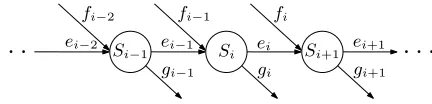
Fig. 1. Illustration of the notation used in Section 3.1. Every node in the shown graph corresponds to a
2-change. The arcs going into a nodeurepresent the edges removed from the tour in stepuand the arcs going out of a nodeurepresent the edges added to the tour in stepu.
PROOF. There are at mostm2 different choices for the first step S
1 because there
are at most m2
≤ m2/2choices for the two edges that are removed from the tour in
stepS1 and, once these are fixed, at most two choices for the edges added to the tour
in step S1 (remember that the edges must form a 4-cycle alternating between edges added and removed from the tour).
OnceSiis fixed, there are at most4mchoices forSi+1because there are two choices
for the edge that linksSiandSi+1, at mostmchoices for the other edge removed from
the tour in stepSi+1, and, once these are fixed, at most two choices for the edges added
to the tour in stepSi+1.
We call a sequence of stepsε-badif every step in the sequence is improving but yields an improvement of at mostε. The probability that a fixed 2-change is an improvement by at most ε is bounded from above by εφ. Ideally we would like to show an upper bound of(εφ)k on the probability that each step in a given linked sequenceS
1, . . . , Sk
is an improvement by at mostε. However, for general linked sequences this is not true because the steps can be dependent in various ways (some steps might even repeat). We need to introduce further restrictions on linked sequences to obtain a good upper bound on the probability that every step is a small improvement.
In the following definitions, we assume that a linked sequenceS1, . . . , Skof 2-changes
is given. Fori∈[k], in stepSithe edgesei−1 andfi−1are removed from the tour and
the edges ei andgi are added to the tour, i.e., for i ∈[k−1], ei denotes an edge that
links the stepsSi andSi+1. These definitions are illustrated in Figure 1.
Definition3.2 (witness sequences of type 1). If for everyi∈[k], the edgeeidoes not
occur in any step Sj with j < i, thenS1, . . . , Sk is called ak-long witness sequence of
type 1.
Ak-long witness sequence of type 1 possesses enough randomness to obtain an upper bound of(εφ)kfor the probability that it isε-bad because every step introduces an edge
that has not occurred in the steps before (see Lemma 3.5).
Definition3.3 (witness sequences of type 2). If for everyi∈[k], the edgeeidoes not
occur in any stepSjwithj < iand if each endpoint offk−1occurs in some stepSjwith
j < k (not necessarily the same for both endpoints), thenS1, . . . , Sk is called ak-long
witness sequence of type 2.
Observe that every k-long witness sequence of type 2 is also a k-long witness se-quences of type 1. Hence, also for every witness sese-quences of type 2, we obtain the desired bound of(εφ)kfor the probability that it isε-bad. Due to the additional
restric-tion onfk−1, the number ofk-long witness sequences of type 2 is at mostk24kmk (see
Lemma 3.5). Even though it seems like a minor detail, it is very important that the exponent ofmin this bound is onlykand notk+ 1as fork-long witness sequences of type 1. The reason why this is important is that, as we will see later, the quotient of the exponents of mandεin the upper bound for the probability that there exists an
[image:7.612.200.416.92.144.2]length of the longest path in the state graph. For witness sequences of type 1 this quo-tient is(k+ 1)/k = 1 + 1/k while it is only k/k = 1for witness sequences of type 2. Since we aim for the exponent1 +o(1), witness sequences of type 1 are only helpful in our analysis fork=ω(1)while witness sequences of type 2 of any length yield a good enough bound on the expected length of the longest path in the state graph.
Definition3.4 (witness sequences of type 3). If for everyi∈[k−1], the edgeei does
not occur in any step Sj with j < i, if ek and gk both occur in steps Sj with j <
k (not necessarily the same), and if fk−1 does not occur in any step Sj with j < k
thenS1, . . . , Sk is called ak-long witness sequence of type 3.
Also every witness sequences of type 3 possesses enough randomness to bound the probability that it isε-bad by(εφ)kbecause every step introduces a new edge. The num-ber of witness sequences of type 3 is bounded from above byk24k+1mk(see Lemma 3.5).
Hence, the same reasoning as for witness sequences of type 2 applies and witness se-quences of type 3 of any length yield a good enough bound on the expected length of the longest path in the state graph.
3.2. Probability of the Existence of a Bad Witness Sequence
In this section, we analyze the probability that there exists an ε-badk-long witness sequence.
LEMMA 3.5. The probability that there exists
a) anε-badk-long witness sequence of type 1 is bounded from above by4k−1mk+1(εφ)k, b) anε-badk-long witness sequence of type 2 is bounded from above byk24kmk(εφ)k,
c) anε-badk-long witness sequence of type 3 is bounded from above byk24k+1mk(εφ)k.
PROOF. a) We considerk-long witness sequences of type 1 first. In accordance with Lemma 3.1 the number of such sequences is at most4k−1mk+1. Now fix an arbitrary
k-long witness sequenceS1, . . . , Sk of type 1. We use the same notation as in Figure 1
to denote the edges involved in this sequence. In the first step, the edgese0andf0are
replaced by the edgese1andg1. As in the proof of Theorem 2.1, we use the principle of deferred decisions and assume that the lengths of the edges e0,f0, andg1 are
de-termined by an adversary. The improvement of step S1can be expressed as a simple linear combination of the lengths of the involved edges. Hence, for fixed lengths ofe0,
f0, andg1, the event thatS1is an improvement by at mostεcorresponds to the event that the length d(e1)of e1 lies in some fixed interval of length ε. Since the density of d(e1) is bounded byφ, the probability that d(e1) takes a value in this interval is
bounded byεφ.
Now we consider a step Si with i ≥ 2 and apply again the principle of deferred
decisions. We assume that arbitrary lengths for the edgesej andfjwithj < iand for
gj withj ≤iare chosen. Since the edgeeiis not involved in any stepSj withj < i, its
length is not determined. Hence, analogously to the first step, the probability that step
Si is an improvement by at mostεis bounded from above byεφfor every realization
of the stepsSj with j < i. Applying this argument to every stepSi yields the desired
bound of(εφ)k. A union bound over all witness sequences of type 1 concludes the proof
of a).
b) Since S1, . . . , Sk−1 is a (k−1)-long witness sequence, there are at most4k−2mk
choices for these steps. The number of different vertices involved in stepsSiwithi < k
is at most 4 + 2(k−2) = 2k because the first step introduces four new vertices and every other step at most two. Since the endpoints of the edge fk−1 must be chosen
among those vertices that have been involved in the stepsSi withi < k, there are at
most 2k
2
<2k2choices forf
the edgeek−1that linksSk−1andSk. If the edgesek−1andfk−1are determined, there
are two choices forekandgk. Hence, in total there are at most8k2possible choices for
stepSk. This implies that the number of differentk-long witness sequences of type 2
is bounded by8k24k−2mk < k24kmk.
Applying the same arguments as for witness sequences of type 1, yields for every witness sequence of type 2 that it is ε-bad only with a probability of at most(εφ)k. A
union bound over all witness sequences of type 2 concludes the proof of b).
c) Since S1, . . . , Sk−1 is a (k−1)-long witness sequence, there are at most 4k−2mk
choices for these steps. The number of different edges involved in stepsSiwith i < k
is at most 4 + 3(k−2) < 3k because the first step introduces four new edges and every other step at most three. Hence, when the steps S1, . . . , Sk−1 are fixed, there
are at most two choices for the edge ek−1 that links Sk−1 and Sk and there are at
most 32k
≤ 9k2/2 choices for the set{e
k, gk}. Onceek−1 and {ek, gk}are fixed, there
are two choices forfk−1. The total number of k-long witness sequences of type 3 can
thus be bounded from above by18k24k−2mk < k24k+1mk.
Similar to witness sequences of type 1, we can bound the probability that a fixed
k-long witness sequence of type 3 isε-bad from above by (εφ)k because also the last step introduces an edge that does not occur in the steps before, namelyfk−1.
Definition 3.6. In the following, we use the termk-witness sequence to denote ak -long witness sequence of type 1 or ani-long witness sequence of type 2 or 3 withi≤k.
Observe that in general a k-witness sequence can contain non-improving 2-changes, which increase the length of the tour. As 2-Opt does not make such 2-changes, we are only interested ink-witness sequences in which every 2-change is improving.
Definition 3.7. We call ak-witness sequenceimprovingif every 2-change in the se-quence is an improvement. Moreover, by ∆(wsk) we denote the smallest total
improve-ment made by any improvingk-witness sequence.
The reason why the previous definition treats witness sequences of type 1 differently than those of type 2 or 3 is that, as discussed above, witness sequences of type 1 are only helpful in our analysis if they are long enough while witness sequences of type 2 or 3 of any length are helpful. Lemma 3.5 shows that it is unlikely that there exists an improvingk-witness sequence whose total improvement is small.
COROLLARY 3.8. For any natural numberk≥3and0< ε≤64m(k−1)/(k−2)φ−1,
PROOF. Due to Lemma 3.5 and the fact that witness sequences of type 2 or 3 must consist of at least two steps, a union bound over allk-witness sequences yields
Prh∆(wsk)≤εi≤4k−1mk+1(εφ)k+ k
X
i=2
i24imi(εφ)i+ k
X
i=2
i24i+1mi(εφ)i
≤4k−1mk+1(εφ)k+ 5 ∞
X
i=2
i2(4mεφ)i
= 4k−1mk+1(εφ)k+ 5· (4mεφ)
2(4−12mεφ+ (4mεφ)2)
(1−4mεφ)3
≤4k−1mk+1(εφ)k+ 5·16
15
3
·(4mεφ)2·4 + 1 162
≤4k−1mk+1(εφ)k+ 25·(4mεφ)2.
Here we used, in the third step, thatP∞
i=1i
2ai= a(a+1)
(1−a)3 for anya∈[0,1). In the fourth
and fifth step, we used that the upper bound onεin the corollary implies4mεφ≤1/16. The above inequality implies the corollary because forε≤ 64m(k−1)/(k−2)φ−1, the second term in the sum is at least as large as the first one.
3.3. Finding Witness Sequences
In the previous section, we have shown an upper bound on the probability that there exists anε-badk-witness sequence. In this section, we show that in every long enough sequence of consecutive 2-changes, one can identify a certain number of disjoint k -witness sequences. In this way, we obtain a lower bound on the improvement made by any long enough sequence of consecutive 2-changes in terms of∆(wsk).
LEMMA 3.9. Letn ≥ 8, k ∈ N, and letS1, . . . , St denote a sequence of consecutive
2-changes performed by the 2-Opt heuristic with t ≥ n4k−1. The sequence S1, . . . , S
t
shortens the tour by at leastt/4k+1·∆(k) ws.
Basically, we have to show that one can findt/4k+1disjointk-witness sequences in the given sequenceS1, . . . , Stof consecutive 2-changes. To do this, we first introduce a
so-calledwitness DAG(directed acyclic graph) which represents the sequenceS1, . . . , St
of 2-changes. In order to not confuse the constructed witness DAG W with the input graph G, we use the terms nodes and arcs when referring to the DAG W and the termsverticesandedgeswhen referring toG. For every stepSi in the given sequence
there is one node inW. Every node has at most two incoming and either zero or two outgoing arcs and every arc is labeled with an edge of the graphG. Consider a node that corresponds to a stepSiin which the edgeseande0 are exchanged with the edges
f andf0. If there exists a stepSj withj > iin which the edge f is removed from the
tour then letj1> idenote the smallest such index, i.e., the edgef is removed from the tour in stepSj1and does not occur in the stepsSi+1, . . . , Sj1−1. Similarly if there exists
a stepSj with j > iin which the edgef0 is removed from tour then letj2 > idenote
the smallest such index. Only if bothj1 andj2 are defined, the node that corresponds
toSihas outgoing arcs. It has one outgoing arc to the node that corresponds toSj1 and
that is labeled with f and it has a second outgoing arc to the node that corresponds toSj2and that is labeled withf
0.
node uis the induced sub-DAG of those nodes of W that can be reached from u by traversing at mostk−1arcs. The following two lemmas directly imply Lemma 3.9.
LEMMA 3.10. Letube a node of height at leastk−1inW. The 2-changes represented by the nodes in the sub-DAGWuyield a total improvement of at least∆
(k) ws.
LEMMA 3.11. Letn≥8. Every witness DAG that represents a sequence oft≥n4k−1
2-changes contains at least t/4k+1 nodes of height at least k−1whose corresponding
sub-DAGs are pairwise disjoint.
PROOF PROOF OF LEMMA3.10. Assume that a sub-DAGWu with rootuof height
at leastk−1 inW is given. Any path from uto some other node in Wu corresponds
to a sequence of 2-changes. LetP be such a path. From the definition ofW it follows that every node onPcorresponds to a stepSiwhere the indices are strictly increasing
alongP(in particular, every node onPcorresponds to a step with a different index). In the following, we show that at least one path inWucorresponds to ak-witness sequence
or a sequence whose total improvement is at least as large as the total improvement of one of thek-witness sequences.
In order to identify such a path, we unroll the sub-DAG Wu to a complete binary
treeT of heightk−1. The root ofT is the nodeuand every node inT whose distance to the root is smaller than k−1 has two children, namely (copies of) its two direct successors inWu. In general, the binary treeT contains multiple nodes that represent
the same stepSi. However, ifP is a downward path inT from the rootuto some other
node, then it is still the case that each node on P corresponds to a stepSi where the
indices are strictly increasing alongP.
Letvbe an inner node ofT, letabe one of its outgoing arcs, letebe the label ofa, and letP be the downward path from the rootuto the nodevinT, not includingv itself. We say that the arcaisnon-continuableif the edgeeoccurs in one of the steps that are represented by the nodes ofP andcontinuableotherwise. (Observe that this does not necessarily mean that one of the arcs on the path fromutovhas labele.) The intuition underlying this definition is as follows: We would like to find a downward path inWu
starting at the root u whose nodes correspond to a witness sequence. Only paths in which all arcs are continuable can correspond to witness sequences of type 1 or 2. For witness sequences of type 3 all arcs except for the last one must be continuable.
Now let v be a leaf ofT. Thenv does not have any outgoing arcs. Nevertheless, as every node ofT, it corresponds to a step in which two edges are added to the tour. We call the leafvnon-continuableif both these edges occur in steps that are represented by the nodes of the downward path from the rootuto the nodev inT, not includingv
itself, andcontinuableotherwise. The intuition underlying this definition is as follows: Any downward path in Wu starting at the root uto a leaf v can only correspond to
a witness sequence of type 1 if all its arcs are continuable and if the leaf v is also continuable.
If T contains a downward path that corresponds to ak-witness sequence of type 1 then we are done. Assume that T does not contain such a path. Then the following property must be true for any path P from the rootuto a leafv of T: at least one of the arcs ofP is non-continuable orvis non-continuable. This is the case because any path fromuto a continuable leafvthat contains only continuable arcs corresponds to a
k-witness sequence of type 1 (the continuable arcs correspond to the edgese1, e2, . . . , ek
ei+1
Si
Si+1
ei
fi gi+1
ei−1
Si−1
gi−1 e
0
i
fi−1
fi−2
ei−2
. . .
e0i+1
S0
i+1
f0
i
gi0+1
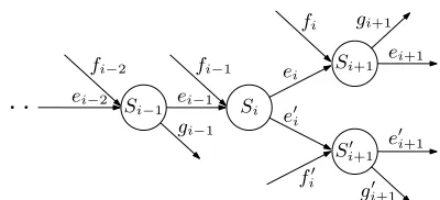
Fig. 2. Summary of our notation. We assume that the nodes corresponding toSi+1andS0i+1are leaf nodes
ofT0and non-continuable.
Let vi+1 be one node with maximum distance from the root in T0 and letvi be its
parent. Let the 2-changes represented by the nodes on the downward path P from the rootutovi+1beS1, . . . , Si+1. Ifvi has two children inT0 then letvi0+1 denote the
child different fromvi+1 and let Si0+1 denote the step that is represented by vi0+1. In
Figure 2, we summarize the notation that we use in the following. In stepSjforj≤i−1
andj=i+1, the edgesej−1andfj−1are exchanged with the edgesejandgj. In stepSi,
the edgesei−1 andfi−1 are exchanged with the edgesei ande0i, and in stepSi0+1, the
edgese0iandfi0are exchanged with the edgesei0+1andg0i+1. We denote byEiall edges
that are involved in stepsSjwithj ≤i. Similarly, byEi−1we denote all edges that are
involved in stepsSj withj≤i−1.
Observe that all leaves inT0 must be non-continuable. For leaves of height smaller than k−1 this follows from the definition ofT0. If any such leafv had a continuable
arc inT then this arc and the corresponding child ofvwould also be contained inT0. Leaves of heightk−1inT0cannot be continuable because otherwise the path to such a leaf would represent ak-witness sequence of type 1, as discussed above. Our construc-tion ensures thatS1, . . . , Siis ani-witness sequence of type 1 because the path from the
rootuto the leafvi+1consists of continuable arcs only. The sequenceS1, . . . , Si+1,
how-ever, is not a witness sequence of type 1 because all leaves ofT0 are non-continuable, which impliesei+1, gi+1∈Ei.
In the following we will shrink the treeT0until a witness sequence of type 2 or 3 is found. For this, we define the operationcontract(Si, Si+1). This operation will only be
applied if the node that corresponds toSihas only a single child inT0(namely the one
that corresponds toSi+1) and if the net effect ofSi andSi+1 together corresponds to a
single 2-changeS. In this case the operationcontract(Si, Si+1)replaces the nodesvi
andvi+1that represent the stepsSiandSi+1by a node the represents the 2-changeS.
We call the tree that results from this operation again T0. The following invariant will remain true throughout the construction: The only nodes that were produced by a contract operation are leaves in the current treeT0. Furthermore each leaf that was
created by a contract operation has the same net effect as the contracted steps and it is non-continuable. For every leaf that was produced by contract operations, the steps contracted form a descending path in the original tree T0 in which every node has at most one child.
The following case analysis shows that it is always possible to either identify a wit-ness sequence of type 2 or 3 or to apply the operationcontract(Si, Si+1). We use the
notationreturnj(R1, . . . , R`)to denote thatR1, . . . , R`is an`-long witness sequence of
typej.
Sincevi+1is non-continuable, we can assumeei+1, gi+1∈Ei.
[image:12.612.208.408.89.180.2]root,v0
i+1must also be a leaf inT0and hence it is also non-continuable due to the
invariant. This is equivalent toe0i+1, gi0+1∈Ei.
(1) Iffi−1∈Ei−1, thenreturn2(S1, . . . , Si).
From now on we assumefi−1∈/Ei−1.
(2) Ife0i∈Ei−1, then consider the following cases.
(a) Iffi ∈/ Ei, thenreturn3(S1, . . . , Si+1).
(b) Ifei+1, gi+1∈Ei−1, thenreturn2(S1, . . . , Si).
S1, . . . , Siis a witness sequence of type 2 because one endpoint offi−1equals one
endpoint ofe0iand the other one equals one endpoint of eitherei+1orgi+1.
(c) Iffi ∈Eiand (ei+1∈Ei\Ei−1orgi+1∈Ei\Ei−1), thencontract(Si, Si+1).
In this case one can assume w.l.o.g. thatgi+1=fi−1andei+1 ∈Ei−1sinceEi\
Ei−1 = {ei, fi−1} and the edges ei, ei+1, and gi+1 are pairwise distinct
be-cause they occur in the same 2-changeSi+1. Thecontract-operation replacesvi
andvi+1by a node that represents the 2-changeS:= (ei−1, fi)→(e0i, ei+1).
(3) Ife0i∈/ Ei−1, thenei+1, gi+1, e0i+1, gi0+1 ∈Ei. Consider the following cases.
(a) If fi ∈/ Ei or fi0 ∈/ Ei, then return3(S1, . . . , Si+1) or return3(S1, . . . , Si, Si0+1),
respectively.
From now on we assumefi, fi0∈Ei.
(b) Ifei+1, gi+1, e0i+1, gi0+1∈Ei−1, thenreturn2(S1, . . . , Si).
S1, . . . , Si is a witness sequence of type 2 due to the invariant and the fact that
the endpoints offi−1coincide with some endpoints ofei+1, gi+1, e0i+1, g0i+1.
(c) If|{ei+1, e0i+1, gi+1, gi0+1} ∩(Ei\Ei−1)| ≥1, then assume w.l.o.g.gi+1∈Ei\Ei−1
andreturn2(S1, . . . , Si−1, S)for the 2-changeS defined below.
In this case Ei\ Ei−1 = {ei, e0i, fi−1}. Furthermore, ei+1 6= e0i and gi+1 6= e0i
because ei+1 and gi+1 both share one endpoint with ei whereas e0i and ei do
not share any endpoints. Furthermore, the edgesei,ei+1, andgi+1are pairwise
distinct because they occur in the same 2-changeSi+1. As in case 2 (c), we assume
w.l.o.g. thatgi+1=fi−1andei+1∈Ei−1.
It must befi 6=e0i as otherwise stepSi would be reversed in stepSi+1.
Further-more, the edgesfi,ei, and,fi−1=gi+1are pairwise distinct because they occur in
the same 2-changeSi+1. Hence,fi∈Ei−1. For the stepS:= (ei−1, fi)→(e0i, ei+1),
the sequenceS1, . . . , Si−1, S is a witness sequence of type 2 because fi ∈ Ei−1
ande0i ∈/ Ei−1. Observe that the original sequenceS1, . . . , Si+1 yields the same
net effect and hence the same improvement as the sequenceS1, . . . , Si−1, S.
If the operation contract(Si, Si+1) is performed in Case 2 (c) then the invariant
stays true. If the nodevi+1was not created by a previous contraction this follows
eas-ily because Case 2 is only reached if vi has only one child and contract(Si, Si+1)
re-placesviandvi+1 by a node that represents the 2-change(ei−1, fi)→(ei+1, e0i), which
is the net effect ofSiandSi+1together. Furthermoreei+1, e0i∈Ei−1and hence the new
node is non-continuable. With the same arguments it also follows that the invariant stays true if the nodevi+1was created by previous contractions.
We repeatedly apply the case analysis above to a node in T0 with maximum distance to the root until a witness sequence is found. Observe that the opera-tion contract(Si, Si+1)is only performed in Case 2 (c) and that each time it is
per-formed the number of nodes in T0 decreases by one. Furthermore it is not possible
thatT0 shrinks to a single node because this node would be a leaf that must be non-continuable due to the invariant. However, the root ofT0is always continuable because there are no previous steps in which the edges added to the tour can occur. Hence after finitely many occurrences of the operation contract(Si, Si+1)one of the other cases
The witness sequence returned is in general not a sequence of steps that are con-tained in the DAGWubecause the last stepS (and only the last step) in the returned
sequence is potentially the result of some contract operations. This is, in particular, true for Case 3 (c) in which the steps Si and Si+1 are contracted without explicitly
calling the operation contract. Due to the invariant, we know that the steps that are contracted into the last step S have the same net effect asS. Furthermore these steps have pairwise distinct indices because they lie on a downward path inT. So the improvement of every step is counted at most once. Hence, the improvement of the witness sequence returned always equals the total improvement of some steps that are contained inWu. This concludes the proof.
PROOF PROOF OFLEMMA3.11. Let W be a witness DAG that consists oftnodes that represent the steps S1, . . . , St. By definition a node in W has either two direct
successors or none at all. The case that a node has no successors can only occur if at least one of the edges that is added to the tour in the corresponding step is not removed anymore in later steps. Since the final tour that is obtained after performing the stepsS1, . . . , Stcontains exactlynedges, at mostnof the nodes ofW can be leaves.
HenceW contains at leastt−nnodes with two outgoing arcs.
We defined the height of a nodevinW to be the minimum distance fromvto one of the leaves ofW. Since every node in W has an indegree of at most two, there are at most n2k−1 nodes inW whose height is smaller thank−1. Hence, there are at least t−n2k−1 nodes inW with an associated sub-DAG of depthk−1. We construct a set
of disjoint sub-DAGs in a greedy fashion: We take an arbitrary sub-DAGWu and add
it to the set of disjoint sub-DAGs that we construct. After that, we remove all nodes of Wufrom the DAGW. We repeat these steps until no complete sub-DAG Wuis left
inW.
In order to see that the constructed set consists of at leastt/4k+2disjoint sub-DAGs, observe that each sub-DAG of depthk−1contains at most2k−1 nodes because the
outdegree of every node is at most two. Each node can be contained in at most2k−1
sub-DAGs of depth k−1 because the indegree of every node is at most two. Hence, every sub-DAG Wu can only intersect with at most(2k−1)2 ≤ 4k other sub-DAGs.
Thus, the number of pairwise disjoint sub-DAGs must be at least
t−n2k−1
4k
≥
t/2
4k
≥ t
4k+1,
where both inequalities follow from the assumptiont≥n4k−1. For the second
inequal-ity we additionally used the assumptionn≥8.
3.4. The Expected Number of 2-Changes
Now we can prove Theorem 1.1.
PROOF PROOF OFTHEOREM1.1. We combine Corollary 3.8 and Lemma 3.9 to ob-tain an upper bound on the probability that the length T of the longest path in the state graph exceedst. Letn≥8. Fort ≥n4k−1, the tour is shortened by the sequence of 2-changes by at leastt/4k+1·∆ws(k). Hence, fort≥n4k−1,
Pr[T ≥t]≤Pr
t
4k+1 ·∆ (k) ws ≤n
=Pr
∆(wsk)≤n4
k+1
t
.
Combining this inequality with Corollary 3.8 yields fort≥t0:=d4k+4nm(k−1)/(k−2)φe,
Pr[T ≥t]≤800
4k+1nmφ
t 2
Note that the restrictiont ≥t0 is necessary to apply Corollary 3.8. We can bound the
expected number of 2-changes as follows:
E[T] = ∞
X
t=1
Pr[T ≥t]≤t0+ ∞
X
t=t0+1
800
4k+1nmφ
t 2
≤t0+
Z ∞
t0
800
4k+1nmφ
t 2
dt
≤t0+800(4
k+1nmφ)2
t0
=O4knm(k−1)/(k−2)φ.
Settingk=√lnmyields
E[T] =O4 √
lnmm√ 1
lnm−2nmφ
=O42 √
lnmnmφ,
where the last equation holds for sufficiently largem.
4. UPPER BOUND FOR THE SECOND MOMENT
Our method does not yield strong concentration bounds for the expected length of the longest path in the state graph. The reason is that the exponent ofεin Corollary 3.8 is only 2. It is, however, possible to bound the second moment ofT.
THEOREM 4.1. For everyφ-perturbed graph withnvertices andmedges
E
T2=O
16 √
lnm
mφ 2
·n3
.
PROOF. The proof follows along the same lines as the proof of Theorem 1.1. Letn≥
8. Fort≥n4k−1, the tour is shortened by the sequence of 2-changes by at leastt/4k+1·
∆(wsk). Hence, fort≥n4k−1,
Pr T2≥t
=PrhT ≥√ti≤Pr
√t
4k+1·∆ (k) ws ≤n
=Pr
∆(wsk)≤n4
k+1
√
t
.
Combining this inequality with Corollary 3.8 yields for t ≥ t0 := (d4k+4nm(k−1)/(k−2)φe)2,
PrhT ≥√ti≤800
4k+1nmφ
√
t 2
Note that the restrictiont≥t0is necessary to apply Corollary 3.8. Using thatT2cannot
be larger than(n!)2, we can bound the expected value ofT2as follows:
E T2=
(n!)2
X
t=1
Pr T2≥t
≤t0+
(n!)2
X
t=t0+1
800
4k+1nmφ
√
t 2
≤t0+
Z (n!)2
t0
800
4k+1nmφ
√
t 2
dt
≤t0+ 800(4k+1nmφ)2
Z (n!)2
1
1
t dt
≤t0+ 800(4k+1nmφ)2·ln((n!)2)
=O
4knm(k−1)/(k−2)φ 2
nln(n)
.
Settingk=√lnmyields
E
T2=O
4 √
lnmm√ 1
lnm−2nmφ
2 nln(n)
=O
16 √
lnmnmφ2n
,
where the last equation holds for sufficiently largem. Let B = c·16
√
lnmnmφ, wherec is the constant from the Big O notation in
Theo-rem 1.1. Then Markov’s inequality implies for every a ≥ 1 that Pr[T ≥aB] ≤ 1/a. Theorem 4.1 implies the following concentration bound, which is stronger for largea.
COROLLARY 4.2. If m is sufficiently large, there exists a constant κ such thatPr[T ≥aB]≤nκ/a2for anya≥1.
PROOF. Letκbe chosen such thatE
T2≤κB2n. Such a constantκmust exist due to Theorem 4.1. Then
Pr[T ≥aB] =Pr
T2≥a2B2=Pr
T2≥ a
2
nκκB 2n
≤ nκ
a2,
which proves the corollary.
REFERENCES
Barun Chandra, Howard J. Karloff, and Craig A. Tovey. 1999. New Results on the Oldk-Opt Algorithm for the Traveling Salesman Problem.SIAM J. Comput.28, 6 (1999), 1998–2029.
Matthias Englert, Heiko R¨oglin, and Berthold V¨ocking. 2014. Worst Case and Probabilis-tic Analysis of the 2-Opt Algorithm for the TSP. Algorithmica 68, 1 (2014), 190–264.
DOI:http://dx.doi.org/10.1007/s00453-013-9801-4
David S. Johnson and Lyle A. McGeoch. 1997. The Traveling Salesman Problem: A Case Study in Local Optimization. InLocal Search in Combinatorial Optimization, E. H. L. Aarts and J. K. Lenstra (Eds.). John Wiley and Sons, New York, NY, USA.
Walter Kern. 1989. A Probabilistic Analysis of the Switching Algorithm for the Euclidean TSP. Mathemati-cal Programming44, 2 (1989), 213–219.
George S. Lueker. 1975. Unpublished Manuscript. (1975). Princeton University.
Bodo Manthey and Rianne Veenstra. 2013. Smoothed Analysis of the 2-Opt Heuristic for the TSP. InProc. of the 24th International Symposium on Algorithms and Computation (ISAAC). Springer, Berlin, 579–589. Daniel A. Spielman and Shang-Hua Teng. 2004. Smoothed Analysis of Algorithms: Why the Simplex