Decaying and decayless transverse oscillations of a coronal loop

warwick.ac.uk/lib-publications

Original citation:

Nisticò, Giuseppe, Nakariakov, V. M. (Valery M.) and Verwichte, E. (Erwin). (2013) Decaying

and decayless transverse oscillations of a coronal loop. Astronomy & Astrophysics, 552 . A57.

Permanent WRAP URL:

http://wrap.warwick.ac.uk/62809

Copyright and reuse:

The Warwick Research Archive Portal (WRAP) makes this work by researchers of the

University of Warwick available open access under the following conditions. Copyright ©

and all moral rights to the version of the paper presented here belong to the individual

author(s) and/or other copyright owners. To the extent reasonable and practicable the

material made available in WRAP has been checked for eligibility before being made

available.

Copies of full items can be used for personal research or study, educational, or not-for-profit

purposes without prior permission or charge. Provided that the authors, title and full

bibliographic details are credited, a hyperlink and/or URL is given for the original metadata

page and the content is not changed in any way.

Publisher’s statement:

“Reproduced with permission from Astronomy & Astrophysics, © ESO”.

A note on versions:

The version presented here may differ from the published version or, version of record, if

you wish to cite this item you are advised to consult the publisher’s version. Please see the

‘permanent WRAP URL’ above for details on accessing the published version and note that

access may require a subscription.

CV4 7AL, UK e-mail:[email protected]

2 _{Central Astronomical Observatory at Pulkovo of the Russian Academy of Sciences, St}

Peters-burg 196140, Russia

Received February 12, 2013/Accepted dd mm yyyy

ABSTRACT

Aims.We investigate kink oscillations of loops observed in an active region with the Atmospheric

Imaging Assembly (AIA) instrument on board the Solar Dynamics Observatory (SDO) spacecraft

before and after a flare.

Methods. The oscillations were depicted and analysed with time-distance maps, extracted from

the cuts taken parallel or perpendicular to the loop axis. Moving loops were followed in time

with steadily moving slits. The period of oscillations and its time variation were determined by

best-fitting harmonic functions.

Results. We show that before and well after the occurrence of the flare, the loops experience

low-amplitude decayless oscillations.The flare and the coronal mass ejection associated to it

trigger large-amplitude oscillations that decay exponentially in time. The periods of the kink

oscillations in both regimes (about 240 s) are similar. An empirical model of the phenomenon in

terms of a damped linear oscillator excited by a continuous low-amplitude harmonic driver and

by an impulsive high-amplitude driver is found to be consistent with the observations.

Key words. Sun: corona - Sun: oscillations - methods: observational

1. Introduction

Transverse, or kink, oscillations of solar coronal loops are among the most often studied dynamical

phenomena in the corona since their discovery (Aschwanden et al. 1999; Nakariakov et al. 1999)

with the Transition Region and Coronal Explorer (TRACE) (Handy et al. 1999). These

oscilla-tions are confidently detected with high-resolution extreme ultra-violet (EUV) imagers, such as the

et al. 2012), and before they were discovered, they were the subject of theoretical and numerical

studies (e.g. Edwin & Roberts 1983; Roberts et al. 1984; Murawski & Roberts 1994). The common

observational manifestation of transverse oscillations are flare-generated rapidly decaying standing

global modes (e.g. Nakariakov et al. 1999) or higher spatial harmonics (Verwichte et al. 2004; De

Moortel & Brady 2007; Van Doorsselaere et al. 2007), but they have been observed as propagating

waves in quiescent active regions (Tomczyk et al. 2007) and in supra-arcades of flaring arcades

(Verwichte et al. 2005). Typical periods of kink oscillations range from a few minutes to several

hours (e.g. White & Verwichte 2012; Verwichte et al. 2010) (the latter case corresponds to cool

fibrils of quiescent prominences, Hershaw et al. 2011). In terms of magnetohydrodynamic (MHD)

wave theory kink oscillations are interpreted as kink (m = 1) fast magnetoacoustic modes (e.g.

Edwin & Roberts 1983; Van Doorsselaere et al. 2008), which become weakly compressible in the

long-wavelength limit (Goossens et al. 2012).

The interest in kink oscillations of coronal loops is mainly connected with their use as a

seis-mological probe of the absolute value of the magnetic field (Nakariakov & Ofman 2001), and also

with their peculiarly rapid damping after excitation (e.g. Ruderman & Roberts 2002; Goossens

et al. 2002). It has been demonstrated that the damping can be caused by resonant absorption, that

is, linear coupling of the kink oscillations with unresolved torsional motions. Standing kink

oscil-lations can be excited by an impulsive, flare-generated driver (e.g. McLaughlin & Ofman 2008), by

a periodic driver associated with a coronal wave (Ballai et al. 2008; Selwa et al. 2010), or directly

from reconnection (White et al. 2012). Alternative mechanisms, e.g. the effect of Alfvénic

vor-tex shedding (e.g. Nakariakov et al. 2009) are also considered. Moreover propagating kink waves

show rapid decay with height, which is believed to be consistent with the resonant absorption

the-ory (Terradas et al. 2010; Pascoe et al. 2010; Verth et al. 2010). Verifying the theories requires

detailed, high-precision observations of this phenomenon.

In this work we present an observation of two different regimes of transverse oscillations,

low-amplitude decay-less and high-low-amplitude decaying, in the same EUV loop.

2. Observations

The analysed coronal loops were observed on the south-eastern solar limb on 30 May, 2012,

be-tween 08:00–11:00 UT with AIA on board SDO, which provides full-disk images of the Sun at

different EUV wavelengths at high spatial resolution (1 pixel _≈0.6 arcsec) every 12 s for each

bandpass. The loop plane is almost parallel to the line-of-sight. The loops were visible in

al-most all six EUV wavelengths: their appearance is weak at 94 and 335 Å, while in 131, 171, 193,

and 211 Å they are clearly visible (better at 171 and 193 Å). This indicates that the loops have a

thermal distribution of about 0.8 and 2 MK. The system of multi-thermal coronal loops belongs

to the active region (AR) NOAA 11494, which was still behind the solar limb at the time of the

observations and emerged only two days later, additionally exhibiting a sunspot. The AR was also

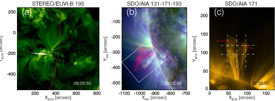
Observa-Fig. 1. (a) Image of the AR NOAA 11494 and the flare from STEREO/EUVI-B at 195 Å: the red line marks the position of the solar limb as seen from the SDO (or Earth). (b) RGB (red, green, blue) image of 131, 171, and 193 Å snapshots from the SDO at the time of the flare: the release of the plasma bubble after the flare is visible in the red (131) channel. (c) Adaptation of the white rectangle in (b) at 171 Å showing the loop system with the overplotted slits (white and red continuous lines). The movie available in the on-line edition shows the temporal evolution of the RGB image of the white rectangle in panel (b) and the time evolution of panel (c). The movie also contains the time-distance maps shown in Fig. 3.

tory (STEREO)-B, which was distant by a few degrees from the solar limb, as seen from the Earth

perspective (the red line in Fig 1a). We cannot appreciate all fine details as seen from SDO, since

the spatial resolution is lower (1 pixel_≈1.6 arcsec), and the identifications of the same loops are

quite difficult at 195 Å (plasma temperature response_≈1.5 MK). At the time of the observations,

a flare occurred in the AR: the typical bright breadth of pixels saturated in intensity was recorded

at 09:05 UT in EUVI-B. The GOES observatories registered a flare of class C1.0 during the time

interval 08:36–09:07 UT. Several minutes later, post-flare loops developed at the right side of the

loop system, and they were visible at EUV wavelengths. A view from SDO is given in Fig. 1b:

we combined three different EUV bandpasses, 131, 171, and 193 Å, respectively in the red, green,

and blue (RGB)channels of the image. This allows us to depict the plasma dynamics at different

temperature ranges. The response functions of the 171 and 193 filters show peaks around 1 MK,

while the 131 channel has a response function peaking at 0.5 MK and 10 MK. While loops are

better visible in the first two filters, the flare is clearly observed at 131 Å, as well as the release of

the plasma bubble, that looks a coronal mass ejection (CME). This release is also recorded in the

hot channels at 94 and 335 Å (but in the latter case it is not seen in “emission”), indicating that

the plasma is probably heated at temperatures around_∼10 MK. The coronal loops are enclosed

inside the white box, and an adaptation of it is shown in Fig. 1c at 171 Å, a few minutes before

the flare. When the flare occurs, transverse oscillations of the loops are triggered, which decay

within about 20 min. Moreover, a careful inspection of the loops shows that transverse oscillations

of smaller amplitude are present before the flare and also after the impulsive event (see movie

on-line). Furthermore, a loop at the right side of the system is increasing its height in time, clearly

showing small-amplitude oscillations before the flare. Here, we focus on the AIA 171 Å dataset.

We selected a box containing the loops that has vertices (starting from the left bottom corner) of

(₋1057.5,₋903.3)] arcsec: the box is 172.8 arcsec wide and 222.6 arcsec high. We extracted it

from the full images, straightened them up as in Fig. 1c, and analysed them.

3. Analysis and results

To study the transverse oscillations, we took slits more or less parallel and perpendicular to the

loop plane and 11-pixel-wide (white lines in Fig. 1c), at positions XBOX =48,72,96 arcsec, and

YBOX =96,120 arcsec, in a similar way as in previous works (e.g. Hershaw et al. 2011; Verwichte

et al. 2004; White & Verwichte 2012). We calculated a mean value over the width at every position

along the slit to increase the signal-to-noise ratio. By stacking slits at every time step (every_∼12

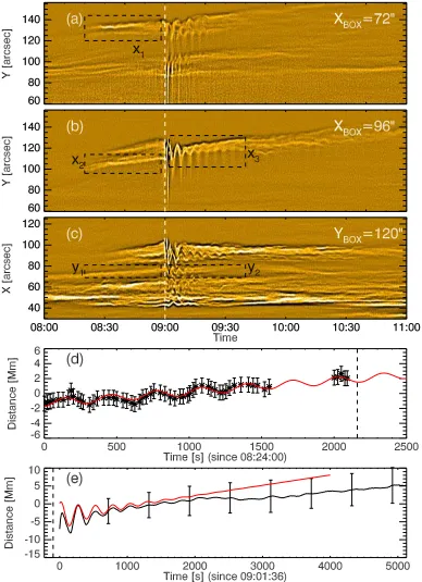
s), we created time-distance plots, that show the intensity variation in time along the slit (Fig. 2).

A decaying wave-like pattern is evident, indicating a periodic displacement of the loop after the

flare, whose time is marked with a white dashed line. At first glance we can note that some static

bright features are present as well, which suggests that some loops do not oscillate (or maybe have

small-amplitude oscillations that are not resolved). In Fig. 2a₋b, we see that the oscillations

are more pronounced at higher distance from the footpoints, indicating that the loop tops oscillate

more than the middle part. A similar behaviour was found for the horizontal slits (Fig. 2c), whose

amplitude is larger at the right side (top oscillations in the time-distance maps) of the loop system

(also closer to the flare site). The CME related to these oscillations shows a speed estimated to

be more than 450 km s−1 _{from AIA-131 data. In addition, decayless oscillations with smaller}

amplitudes are displayed 30 min before and after the flare (e.g. see Fig. 2a–c). Time series of the

loop displacement were extracted from the time-distance maps with a Gaussian fit of the intensity

profile or by eye inspection, and were fitted with the function

y(t)=ξcos 2π(t−t0)

P −φ

! exp

−t−t0 τ

+f (t), (1)

where f (t) is a steady trend (typically linear) in the loop displacement ( f (t)=y0+v0t). Parameters

estimated from the fits are reported in Table 1. The typical oscillation period ranges between 200–

300 s (Fig. 2 f₋g, Table 1), and the decay time is about 500 s. This ratio of the period to the decay

time is typical for decaying kink oscillations (e.g. White & Verwichte 2012).

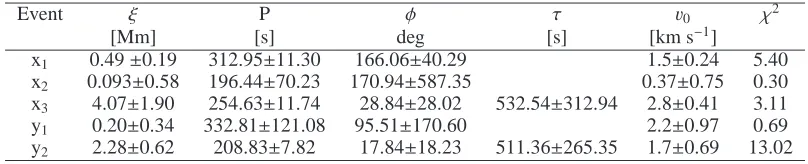
Table 1. Fitting parameters of transverse loop oscillations.

Event ξ P φ τ v0 χ2

[Mm] [s] deg [s] [km s−1]

x1 0.49±0.19 312.95±11.30 166.06±40.29 1.5±0.24 5.40

x2 0.093±0.58 196.44±70.23 170.94±587.35 0.37±0.75 0.30

x3 4.07±1.90 254.63±11.74 28.84±28.02 532.54±312.94 2.8±0.41 3.11

y1 0.20±0.34 332.81±121.08 95.51±170.60 2.2±0.97 0.69

y2 2.28±0.62 208.83±7.82 17.84±18.23 511.36±265.35 1.7±0.69 13.02

To take into account the variation in size of the loop and their direction, we focused on the

expanding loop at the right of the system: we took a slit located at the top of the loop and moved

Fig. 2. High-pass-filtered time-distance maps (a−c) obtained from the slits. Transverse oscillations are

enclosed by the black dashed boxes. Time series plots (d−e) and associated fits (red lines) for events x1, and x3. The white (black) dashed lines in the time-distance maps (time series plots) represent the time of the flare.

different phases (low-large-low amplitude oscillations, which show decayless-decaying-decayless

behaviour). The slit during the first phase was moved faster (the speed of the expanding loop is

estimated to be about 10 km s−1_{) than in the second, and in the last phase it was kept stable since}

the loop height did not seem to change considerably (see on-line movie). We compared this also

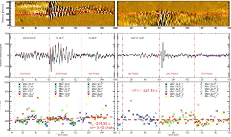
Fig. 3. Top: time-distance maps for the moving (left panel) and steady (right panel) slit (red lines in Fig. 1c). The time distance map of the top left panel is included in the on-line movie; it shows the loop evolution. Middle: Zoomed parts of the time-distance maps: the red and blue bullet are the maxima and minima positions. Bottom: Periodvs time as inferred from the intensity profiles above (red lines in the

time-distance maps). The vertical dot-dashed lines show the different oscillation regimes. The dashed line shows the linear trend in the period, with the initial value about 214 s and the increment of 0.43 s/min (left panel), and the average period of 224.19 s (right panel).

the time-distance maps obtained is given in Fig. 3 (top). A running difference of five frames was

subtracted from the signal to highlight the oscillations: a pattern with recurring dark and bright

spots was obtained by this operation. We also analysed the period changes in time by counting the

maxima (red bullet) and minima (blue bullet) in the intensity profile, taken at a specific cut in the

time-distance maps (Fig. 3, middle). We estimated the period by evaluating the time between the

consecutive maxima (or minima) peaks. Scatter plots of the measured period in time are given in

Fig. 3 (bottom). For the moving slit, we note that the period is initially about 200 s, then it abruptly

increases to 300 s (possibly because of the interaction with another loop at 193 Å), then decreases

and again increases to 300 s during the large-amplitude phase. A similar behaviour is noted in the

third phase, when the loop height is higher than in the first case. From the right scatter plot (fixed

slit), no clear trend for the period evolution can be inferred: the scatter of data is larger than in the

previous one, and the average period is 224.19 s.

We estimated the magnitude of the magnetic field with coronal seismology. The length of the

loops is inferred by considering the two views from STEREO-B and SDO to determine the “true”

length and not just the projection on the plane of sight. In addition, we used difference images to

recognise by eye the brightness variation and associated them to the same loop (see on-line movie).

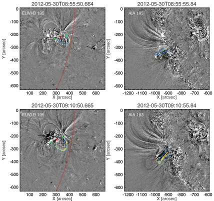
Fig. 4. Three-dimensional reconstruction of two distinct loops before (top) and after (bottom) the flare, projected on the EUVI-B (left) and AIA (right) view. We plotted the centre of the loop (red point) on the solar surface, and the footpoints (green points) on the respective sides. The red line in STEREO-B images represents the limb as seen from the SDO. The points obtained fromscc_measure.proare plotted as yellow dots and the loop profile is given by a blue line. The movie available in the on-line edition shows the temporal evolution of the loops.

the footpoints in EUVI-B, and compared the 3D positions resulting from thescc_measure.pro

with a semi-elliptical profile, which matches the loop shape well. The results are given in Fig. 4.

By knowing the loop length and the period, we can estimate the phase speed (or kink speed),

and consequently the Alfvén speed, as

CK=

s 2 1+ρe

ρ0

VA0≈

2L

P, (2)

withρeandρ0 the external and internal density, and VA0the internal Alfén speed. Since the

density contrast can change between 0 and 1, the Alfvén speed will range between a lower and an

cgs units)

B=VA

q

4πµCmpne, (3)

withµCthe mean molecular weight in the corona, which is equal to 1.27, mpis the proton mass,

and nethe electron density. From the value range of the Alfvén speed, the corresponding magnetic

field is estimated as (see Nakariakov & Ofman 2001; White & Verwichte 2012)

2L

√

2P

√_µ

Cmpne≤B≤

2L P

√_µ

Cmpne. (4)

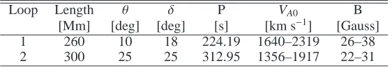
Table 2. Seismological diagnostic

Loop Length θ δ P VA0 B

[Mm] [deg] [deg] [s] [km s−1_{] [Gauss]}

1 260 10 18 224.19 1640–2319 26–38

2 300 25 25 312.95 1356–1917 22–31

In Table 2 we report the parameters of the loop such as length, inclination, and azimuth angle,

the period associated to these loops and the associated Alfén speed as weel as an estimate of the

magnetic field. The values agree with those given in the literature.

4. Discussion and conclusions

There are two different oscillation regimes, one with a decayless low-amplitude and one with a

decaying high-amplitude, suggests that the same resonator (the loop) is excited by two different

drivers. We modelled the observed oscillations with an externally driven damped-driven oscillator

d2_ξ

dt2 +2γ

dξ

dt +ω

2

0ξ = a0e−iωt+a1δ(t−t0), (5)

where ξ(t) is the transverse displacement of the loop,ω0 is the natural frequency of the global

kink mode (ω0 =CKπ/L, with CKthe kink speed, and L the loop length),γis the damping rate,

e.g. due to resonant absorption. The observations suggest that the oscillation is not over-damped,

i.e. γ < ω0. The right-hand side of Eq. (5) contains a continuous low-amplitude harmonic driver

of the amplitude a0 and frequencyω, and an impulsive driver of the amplitude a1 at the time t0.

The driven solution of Eq. (5) is a superposition of the harmonic low-amplitude signal, and an

impulsively induced decaying oscillation,

ξ(t) = _q a0 cos(ωt−φ) (ω2

0−ω2)2+4γ2ω2

+ a1e−γ(t−t0) cos (Ω(t−t0)) H(t−t0), (6)

whereΩ = q_|ω2 0−γ

2_|andφ=tan−1_(2γω/(ω2 0−ω

2_{)) and H(x) is the Heaviside function.}

Compar-ing the empirically determined behaviour of the loop, Eq. (1), with the damped oscillation (6), we

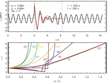
Fig. 5. Top: example displacementξ(t) using Eq. (6) as a function of time, which satisfies condition (7). The amplitudes are a0 =2 Mm and a1 =4 Mm. The two oscillations are in phase. The grey curve shows

the impulsive part. The red line is the fitted damped oscillation (1). Bottom:τγas a function of the ratio of amplitudes a0/a1for different phase differences between the two solutions in Eq. (6). Here a0represents the

full amplitude of the driven oscillation (including the square-root denominator). We assumedω0=2π/250 rad s−1_{,ω=2π/200 rad s}−1_{,γ=1/530 Hz.}

magnitude of the decrease in the oscillation amplitude depends on the specific values of a0, a1and

γ. Fig. 5-bottom shows the decrease in the observed amplitude for short-phase differences between

the harmonically and impulsively driven oscillations and for the amplitude ratio a0/a1≈0.5 (here

a0 represents the full amplitude of the driven oscillation, including the square-root denominator).

This behaviour is consistent with the one shown in Fig. 3 (middle).

Our observations also showed that the loop gradually expands, which might affect the natural

frequencyω0. By assuming mass conservation and a constant cross-section of the loop in time,

the length L grows by dL, and the mass densityρdecreases asρ/(1+dL/L). Since the period of

P = P0+dP = P0(1+dL/L)

1

2/(1+dB/B), where P₀ is the initial value, in our case P₀ ∼215

s. Indeed, given an increase in height of the loop from 51 to 84 arcsec, and assuming dB=0, the

period is expected to be P=1.28 P0 =275 s. Moreover, the linear fit of the period measurements

(Fig. 3, bottom left) provides an estimate of the growth rate, m=0.43 s/min, leading to a value of

P_∼280 s, which is consistent with the expectations.

Therefore, we interpret the observed two regimes of kink oscillations of a coronal loop as

the response of the loop (which is a dissipative fast magnetoacoustic resonator) to two different

drivers: an external non-resonant harmonic (or possibly, quasi-harmonic) driver and an impulsive

high-amplitude driver. Numerical approaches have been made to study the behaviour of loops in

response to periodic or impulsive drivers. Ballai et al. (2008) have found that kink oscillations

generated by a harmonic driver have a dominant period belonging to that of the driver, while for

a non-harmonic driver (modelling a shock wave) the generated oscillations are of natural periods

only. Similar conclusions were reached in Selwa et al. (2010), where the authors pointed out that

in the case of an oscillatory driver with a given frequency, only a small subset of loops will start

to oscillate, i.e. those whose typical period matches that of the driver. This can be inferred from

our time distance maps, where low-amplitude oscillations are sketched for only some loops (e.g.

oscillations x1,y1in Fig. 2), while impulsive excitation generates systematically transverse

pertur-bations in all loops. While the latter is associated with the well-observed flare from STEREO-B,

there is no clear association in observations for the former: at the time of decayless oscillations

there is no flare energy release. This also excludes the possibility of the excitation by a

quasi-monochromatic global coronal wave. Such a quasi-periodicity might appear because of dispersion

caused by random structuring of the coronal plasma (Nakariakov et al. 2005; Long et al. 2011). The

driver responsible for the low-amplitude oscillations before and after the flare should have an

intrin-sic period of 3–5 min (see period estimates of x1, x2, andy1in Table 1). A possible source can be

thought to be the sunspots oscillations, which would be consistent with the empirically established

relationship between three min oscillations in solar flares (Sych et al. 2009). However, we cannot

use active region magnetograms, because it was still behind the limb. Other driving mechanisms

might be unresolved footpoint motions, the effect of granulation, or the effect of periodic Alfvénic

vortex shedding caused by the relative motion of the loop with respect to the background plasma.

Moreover, the expanding loop we observed and analysed offers us an opportunity to test the

va-lidity of theoretical and numerical results. Recently, Ballai & Orza (2012) modelled an expanded

coronal loop in an “empty” corona, showing that period and amplitude increase as the length grows

(the low-amplitude oscillations analysed by us do not show a consistent increase in the amplitude,

which leads us to assume a possible dissipative mechanism in balance with forcing). The

approx-imation of an “empty” corona is very drastic and more efforts are needed to obtain more realistic

results. Our observations in this sense can reveal more about the complex dynamical processes

occurring in the solar corona.

Acknowledgements. The data used here are courtesy of the SDO (NASA) and AIA consortia. The authors would like to

Long, D. M., DeLuca, E. E., & Gallagher, P. T. 2011, ApJ, 741, L21 McLaughlin, J. A. & Ofman, L. 2008, ApJ, 682, 1338

Murawski, K. & Roberts, B. 1994, Sol. Phys., 151, 305

Nakariakov, V. M., Aschwanden, M. J., & van Doorsselaere, T. 2009, A&A, 502, 661 Nakariakov, V. M. & Ofman, L. 2001, A&A, 372, L53

Nakariakov, V. M., Ofman, L., Deluca, E. E., Roberts, B., & Davila, J. M. 1999, Science, 285, 862 Nakariakov, V. M., Pascoe, D. J., & Arber, T. D. 2005, Space Sci. Rev., 121, 115

Pascoe, D. J., Wright, A. N., & De Moortel, I. 2010, ApJ, 711, 990 Roberts, B., Edwin, P. M., & Benz, A. O. 1984, ApJ, 279, 857 Ruderman, M. S. & Roberts, B. 2002, ApJ, 577, 475

Selwa, M., Murawski, K., Solanki, S. K., & Ofman, L. 2010, A&A, 512, A76 Sych, R., Nakariakov, V. M., Karlicky, M., & Anfinogentov, S. 2009, A&A, 505, 791 Terradas, J., Goossens, M., & Verth, G. 2010, A&A, 524, A23

Tomczyk, S., McIntosh, S. W., Keil, S. L., et al. 2007, Science, 317, 1192 Van Doorsselaere, T., Nakariakov, V. M., & Verwichte, E. 2007, A&A, 473, 959 Van Doorsselaere, T., Nakariakov, V. M., & Verwichte, E. 2008, ApJ, 676, L73 Verth, G., Terradas, J., & Goossens, M. 2010, ApJ, 718, L102

Verwichte, E., Foullon, C., & Van Doorsselaere, T. 2010, ApJ, 717, 458 Verwichte, E., Nakariakov, V. M., & Cooper, F. C. 2005, A&A, 430, L65

Verwichte, E., Nakariakov, V. M., Ofman, L., & Deluca, E. E. 2004, Sol. Phys., 223, 77 White, R. S. & Verwichte, E. 2012, A&A, 537, A49

White, R. S., Verwichte, E., & Foullon, C. 2012, A&A, 545, A129